Equivalent relaxations of optimal power flow

Abstract

Several convex relaxations of the optimal power flow (OPF) problem have recently been developed using both bus injection models and branch flow models. In this paper, we prove relations among three convex relaxations: a semidefinite relaxation that computes a full matrix, a chordal relaxation based on a chordal extension of the network graph, and a second-order cone relaxation that computes the smallest partial matrix. We prove a bijection between the feasible sets of the OPF in the bus injection model and the branch flow model, establishing the equivalence of these two models and their second-order cone relaxations. Our results imply that, for radial networks, all these relaxations are equivalent and one should always solve the second-order cone relaxation. For mesh networks, the semidefinite relaxation is tighter than the second-order cone relaxation but requires a heavier computational effort, and the chordal relaxation strikes a good balance. Simulations are used to illustrate these results.

I Introduction

I-A Background

The optimal power flow (OPF) problem seeks an operating point of a power network that minimizes a certain cost, e.g., generation cost, transmission losses, etc. It is a fundamental problem as it underlies many applications such as unit commitment, economic dispatch, state estimation, volt/var control, and demand response. There has been a great deal of research since Carpentier’s first formulation in 1962 [2] and an early solution by Dommel and Tinney [3]; recent surveys can be found in, e.g., [4, 5, 6, 7, 8, 9, 10, 11, 12, 13, 14, 15, 16]. OPF is generally nonconvex and NP-hard. A large number of optimization algorithms and relaxations have been proposed, the most popular of which is linearization (called DC OPF) [17, 18, 19, 20]; See also [21] for a more accurate linear approximation. An important observation was made in [22] that OPF can be formulated as a quadratically constrained quadratic program and therefore can be approximated by a semidefinite program (SDP). Instead of solving OPF directly, the authors in [23] propose to solve its convex Lagrangian dual problem. Sufficient conditions have been studied by many authors under which an optimal solution for the non-convex problem can be derived from an optimal solution of its SDP relaxation; e.g., [24, 25, 26] for radial networks and in [23, 27, 28] for resistive networks. These papers all use the standard bus injection model where the Kirchhoff’s laws are expressed in terms of the complex nodal voltages in rectangular coordinates.

Branch flow models on the other hand formulate OPF in terms of branch power and current flows in addition to nodal voltages, e.g., [29, 30, 31, 32, 33, 34, 35, 36]. They have been mainly used for modeling radial distribution networks. A branch flow model has been proposed in [37] to study OPF for both radial and mesh networks and a relaxation based on second-order cone program (SOCP) is developed. Sufficient conditions are obtained in [34, 38, 39] under which the SOCP relaxation is exact for radial networks.

I-B Summary

Since the OPF problem in the bus injection model is a quadratically constrained quadratic program it is equivalent to a rank-constrained SDP [22, 23]. This formulation naturally leads to an SDP relaxation that removes the rank constraint and solves for a full positive semidefinite matrix. If the rank condition is satisfied at an optimal point, the relaxation is said to be exact and an optimal solution of OPF can be recovered through the spectral decomposition of the positive semidefinite matrix. Even though SDP is polynomial time solvable it is nonetheless impractical to compute for large power networks. Practical networks, however, are sparse. In this paper we develop two equivalent formulations of OPF using partial matrices that involve much fewer variables than the full SDP.

The key idea is to characterize classes of partial matrices that are easy to compute and, when the relaxations are exact, are completable to full positive semidefinite matrices of rank 1 from which a solution of OPF can be recovered through spectral decomposition. One of these equivalent problems leads to an SDP relaxation based on chordal extension of the network graph [40, 41] and the other leads to an SOCP relaxation [42, 43]. In this work, we prove equivalence relations among these problems and their relaxations. Our results imply that, for radial networks, all three relaxations are equivalent and we should always solve the SOCP relaxation. For mesh networks there is a tradeoff between computational effort and accuracy (in terms of exactness of relaxation) in deciding between solving SOCP relaxation or the other two relaxations. Between the chordal relaxation and the full SDP, if all the maximal cliques of a chordal extension of the network graph have been pre-computed offline then solving the chordal relaxation is always better because it has the same accuracy as the full SDP but typically involves far fewer variables and is faster to compute. This is explained in Section II. Chordal relaxation has been suggested in [44, 36] for solving OPF, and SOCP relaxation in the bus injection model has also been studied in [26, 45, 1, 28]. Here we provide a framework that unifies and contrasts these approaches.

In Section III we present the branch flow model of [37] for OPF and the corresponding SOCP relaxation developed in [34, 37]. In Section IV we prove the equivalence of the branch flow model and the bus injection model by exhibiting a bijection between these two models and their relaxations. Indeed the relations among the various problems in this paper, both in the bus injection model and the branch flow model, are established through relations among their feasible sets.

It is important that we utilize both the bus injection and the branch flow models. Even though they are equivalent, some relaxations are much easier to formulate and some sufficient conditions for exact relaxation are much easier to prove in one model than the other. For instance the semidefinite relaxation of power flows has a much cleaner formulation in the bus injection model. The branch flow model especially for radial networks has a convenient recursive structure that not only allows a more efficient computation of power flows e.g. [46, 47, 48], but also plays a crucial role in proving the sufficient conditions for exact relaxation in [49, 50]. Since the variables in the branch flow model correspond directly to physical quantities such as branch power flows and injections it is sometimes more convenient in applications.

In Section V, we illustrate the relations among the various relaxations and OPF through simulations. First, we visualize the feasible sets of a 3-bus example in [51]. Then we compare the running times and accuracies of these relaxations on IEEE benchmark systems [52, 53]. We conclude the paper in Section VI.

I-C Notations

Let $\mathbb{R}$ and $\mathbb{C}$ denote the sets of real and complex numbers respectively. For vectors $x,y\in\mathbb{R}^{n}$, $x\leq y$ denotes inequality componentwise; if $x,y\in\mathbb{C}^{n}$, $x\leq y$ means $\text{Re }x\leq\text{Re }y$ and $\text{Im }x\leq\text{Im }y$. For a matrix $A$, let $A^{H}$ be its hermitian transpose. $A$ is called positive semidefinite (psd), denoted $A\succeq 0$, if it is hermitian and $x^{H}Ax\geq 0$ for all $x\in\mathbb{C}^{n}$. Let $\textbf{i}:=\sqrt{-1}$ and for any set $B$, let $|B|$ denote its cardinality.

II Bus injection model and conic relaxations

In this section we formulate OPF in the bus injection model and describe three equivalent problems. These problems lead naturally to semidefinite relaxation, chordal relaxation, and second-order cone relaxation of OPF. We prove equivalence relations among these problems and their exact relaxations.

II-A OPF formulation

Consider a power network modeled by a connected undirected graph $G(N,E)$ where each node in $N:=\{1,2,\ldots,n\}$ represents a bus and each edge in $E$ represents a line. For each edge $(i,j)\in E$ let $y_{ij}$ be its admittance [54]. A bus $j\in N$ can have a generator, a load, both or neither. Typically the loads are specified and the generations are variables to be determined. Let $s_{j}$ be the net complex power injection (generation minus load) at bus $j\in N$. Also, let $V_{j}$ be the complex voltage at bus $j\in N$ and $|V_{j}|$ denote its magnitude. Bus 1 is the slack bus with a fixed magnitude $|V_{1}|$ (normalized to 1). The bus injection model is defined by the following power flow equations that describe the Kirchhoff’s law:

$$s_{j} = \sum_{k:(j,k)\in E}V_{j}(V_{j}^{H}-V_{k}^{H})y_{jk}^{H}\ \ \ \text{ for }j\in N.$$ (1)

The power injections at all buses satisfy

$$\underline{s}_{j}\leq s_{j}\leq\overline{s}_{j}\ \ \ \ \text{ for }j\in N,$$ (2)

where $\underline{s}_{j}$ and $\overline{s}_{j}$ are known limits on the net injection at bus $k$. It is often assumed that the slack bus (node 1) has a generator and there is no limit of $s_{1}$; in this case $-\underline{s}_{j}=\overline{s}_{j}=\infty$. We can eliminate the variables $s_{k}$ from the OPF formulation by combining (1)–(2) into

$$\underline{s}_{j}\ \ \leq\sum_{k:(j,k)\in E}V_{j}(V_{j}^{H}-V_{k}^{H})y_{jk}^{H}\ \ \leq\ \ \overline{s}_{j}\ \ \ \text{ for }j\in N.$$ (3)

Then OPF in the bus injection model can be formulated in terms of just the $n\times 1$ voltage vector $V$. All voltage magnitudes are constrained:

$$\underline{V}_{j}\leq|V_{j}|\leq\overline{V}_{j}\quad\text{ for }j\in N,$$ (4)

where $\underline{V}_{j}$ and $\overline{V}_{j}$ are known lower and upper voltage limits. Typically $|V_{1}|=1=\underline{V}_{1}=\overline{V}_{1}$. These constraints define the feasible set of the optimal power flow problem in the bus injection model:

$$\mathbb{V}:=\{V\in\mathbb{C}^{n}\ |\ V\text{ satisfies }\eqref{eq:opf.1}-\eqref{eq:opf.2}\}.$$ (5)

Let the cost function be $c(V)$. Typical costs include the total cost of generating real power at all buses or line loss over the network. All these costs can be expressed as functions of $V$. Thus, we obtain the following optimization problem.
Optimal power flow problem $OPF$:

$$\underset{V}{\text{minimize}}\quad\ c(V)$$

$$\text{subject to}\quad\ V\in\mathbb{V}.$$

Since (3) is quadratic, $\mathbb{V}$ is generally a nonconvex set. Thus OPF is nonconvex and NP-hard to solve.

Remark 1.

The OPF formulation usually includes additional constraints such as thermal or stability limits on power or current flows on the lines, or security constraints; see surveys in [4, 5, 6, 7, 8, 11, 12, 13, 14, 15]. Our results generalize to OPF with some of these constraints, e.g., line limits [45, 37]. Our model can also include a shunt element at each bus. We omit these refinements for ease of presentation.

II-B SDP relaxation: $\mathcal{P}_{1}$ and $\mathcal{R}_{1}$

Note that (3) is linear in the variables $W_{jj}:=|V_{j}|^{2}$ for $j\in N$ and $W_{jk}:=V_{j}V_{k}^{H}$ for $(j,k)\in E$. This motivates the definition of a $G$-partial matrix. Define the index set $I_{G}$:

$$I_{G}:=\Bigg{\{}(j,j)\ |\ j\in N\Bigg{\}}\ \bigcup\ \Bigg{\{}(j,k)\ |\ (j,k)\in{E}\Bigg{\}}.$$

A ${G}$-partial matrix $W_{G}$ is a collection of complex numbers indexed by the set $I_{G}$, i.e., $[W_{G}]_{jk}$ is defined iff $j=k\in N$ or $(j,k)\in E$. This is illustrated in Figure 2. For graph $G_{1}$, we have $n=5$ nodes and $I_{G_{1}}=\{(1,1),(2,2),(3,3),(4,4),(5,5),(1,2),(2,1),(2,3),\linebreak[0](3,2),(3,4),(4,3),(1,4),(4,1),(4,5),(5,4)\}$ as shown in Figure 2(a) as a partially filled matrix. For graph $G_{2}$ in Figure 1(b), $I_{G_{2}}$ is represented in Figure 2(b). If $G$ is a complete graph, i.e., every pair of nodes share an edge, then $W_{G}$ is an $n\times n$ matrix.

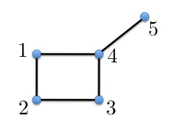
(a) Graph $G_{1}$

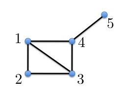
(b) Graph $G_{2}$

Figure 1: Simple graphs to illustrate $G$-partial matrices.

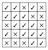
(a) $G_{1}$-partial matrix

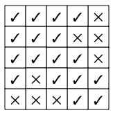
(b) $G_{2}$-partial matrix

Figure 2: Index sets $I_{G_{1}}$ and $I_{G_{2}}$ illustrated as entries in a matrix. Entry $(j,k)$ is marked with a tick if $(j,k)$ is in the corresponding index set; otherwise it is marked with a cross.

The relations in (3)–(4) can be rewritten in terms of $W_{G}$ as:

$$\underline{s}_{j}\leq\sum_{k:(j,k)\in E}\left([W_{G}]_{jj}-[W_{G}]_{jk}\right)y_{jk}^{H}\leq\overline{s}_{j}\;\text{ for }j\in N,$$ (7a)

$$\underline{V}_{j}^{2}\leq[W_{G}]_{jj}\leq\overline{V}_{j}^{2}\;\text{ for }j\in N.$$ (7b)

We assume the cost function $c(V)$ in OPF depends on $V$ only through the $G$-partial matrix $W_{G}$. For instance, if the objective is to minimize the total real power loss in the network then

$$c(V)=\sum_{j\in N}\text{Re }s_{j}=\sum_{j\in N}\sum_{k:(j,k)\in E}\text{Re }\left([W_{G}]_{jj}-[W_{G}]_{jk}\right)y_{jk}^{H}.$$

If the objective is to minimize a weighted sum of real power generation at various nodes then

$$c(V) =\sum_{j\in N}c_{j}\left(\text{Re }s_{j}-p_{j}^{d}\right)$$

$$=\sum_{j\in N}c_{j}\left(\sum_{k:(j,k)\in E}\text{Re }\left([W_{G}]_{jj}-[W_{G}]_{jk}\right)y_{jk}^{H}-p_{j}^{D}\right),$$

where $p_{j}^{d}$ is the given real power demand at bus $j\in N$. Henceforth we refer to the cost function as $c(W_{G})$.

Consider an $n\times 1$ voltage vector $V$. Then $W=VV^{H}$ is an $n\times n$ psd matrix of rank 1. Define the $G$-partial matrix $W(G)$ as the collection of $I_{G}$ entries of $W$. To describe the constraints $V\in\mathbb{V}$, we use the equivalent constraints in terms of $W(G)$ in (7a)-(7b). Formally, OPF is equivalent to the following problem with $n\times n$ Hermitian matrix $W$:
Problem $\mathcal{P}_{1}$:

$$\underset{{W}}{\text{minimize}} c(W(G))$$

subject to $$W(G)\text{ satisfies }\eqref{eq:opfW.1}-\eqref{eq:opfW.2},$$

$${W}\succeq 0,\ \operatorname{\text{rank}}W=1.$$

Given an $V\in\mathbb{V}$, $W=VV^{H}$ is feasible for $\mathcal{P}_{1}$; conversely given a feasible $W$ it has a unique spectral decomposition [55] $W=VV^{H}$ such that $V\in\mathbb{V}$. Hence there is a one-one correspondence between the feasible sets of OPF and $\mathcal{P}_{1}$, i.e., OPF is equivalent to $\mathcal{P}_{1}$. Problem $\mathcal{P}_{1}$ is a rank-constrained SDP and NP-hard to solve. The nonconvex rank constraint is relaxed to obtain the following SDP.
Problem $\mathcal{R}_{1}$:

$$\underset{{W}}{\text{minimize}} c(W(G))$$

subject to $$W(G)\text{ satisfies }\eqref{eq:opfW.1}-\eqref{eq:opfW.2},\quad{W}\succeq 0.$$

$\mathcal{R}_{1}$ is an SDP [56, 43] and can be solved in polynomial time using interior-point algorithms [57, 58]. Let $W^{*}$ be an optimal solution of $\mathcal{R}_{1}$. If $W^{*}$ is rank-1 then $W^{*}$ also solves $\mathcal{P}_{1}$ optimally. We say the relaxation $\mathcal{R}_{1}$ is exact with respect to $\mathcal{P}_{1}$ if there exists an optimal solution of $\mathcal{R}_{1}$ that satisfies the rank constraint in $\mathcal{P}_{1}$ and hence optimal for $\mathcal{P}_{1}$.

Remark 2.

In this paper we define a relaxation to be exact as long as one of its optimal solutions satisfies the constraints of the original problem, even though a relaxation may have multiple optimal solutions with possibly different ranks. The exactness of $\mathcal{R}_{1}$ in general does not guarantee that we can compute efficiently a rank-1 optimal $W_{*}$ if non-rank-1 optimal solutions also exist. Many sufficient conditions for exact relaxation in the recent literature, however, do guarantee that every optimal solution of the relaxation is optimal for the original problem, e.g., [59, 60, 61, 28] or they lead to a polynomial time algorithm to construct an optimal solution of $\mathcal{P}_{1}$ from any optimal solution of the relaxation, e.g., [62, 45].

II-C Chordal relaxation: $\mathcal{P}_{ch}$ and $\mathcal{R}_{ch}$

To define the next relaxation we need to extend the definitions of Hermitian, psd, and rank-1 for matrices to partial matrices:

1. The complex conjugate transpose of a $G$-partial matrix $W_{G}$ is the $G$-partial matrix $(W_{G})^{H}$ that satisfies

   $$[(W_{G})^{H}]_{jk}=[W_{G}]_{kj}^{H}\text{ for all }(j,k)\in I_{G}.$$

   We say $W_{G}$ is Hermitian if $W_{G}=(W_{G})^{H}$.

2. A matrix $M$ is psd if and only if all its principal submatrices (including $M$ itself) are psd. We extend the definition of psd to $G$-partial matrices using this property. Informally a $G$-partial matrix is said to be psd if, when viewed as a partially filled $n\times n$ matrix, all its fully-specified principal submatrices are psd. This notion can be formalized as follows. A clique is a complete subgraph of a given graph. A clique on $k$ nodes is referred to as a $k$-clique. For the graph $G_{1}$ in Figure 1(a), the cliques are the edges. For the graph $G_{2}$ in Figure 1(b), the cliques consist of the edges and the triangles $\{1,2,3\}$ and $\{1,3,4\}$. A $k$-clique $C$ in graph $G$ on nodes $\{n_{1},n_{2},\ldots,n_{k}\}$ fully specifies the $k\times k$ submatrix $W_{G}(C)$:

   $$W_{G}(C)=\begin{pmatrix}[W_{G}]_{n_{1}n_{1}}&[W_{G}]_{n_{1}n_{2}}&\cdots&[W_{G}]_{n_{1}n_{k}}\\ [W_{G}]_{n_{2}n_{1}}&[W_{G}]_{n_{2}n_{2}}&\cdots&[W_{G}]_{n_{2}n_{k}}\\ \vdots&\vdots&\ddots&\vdots\\ [W_{G}]_{n_{k}n_{1}}&[W_{G}]_{n_{k}n_{2}}&\cdots&[W_{G}]_{n_{k}n_{k}}\end{pmatrix}.$$

   We say a $G$-partial matrix $W_{G}$ is positive semidefinite (psd), written as $W_{G}\succeq 0$, if and only if $W_{G}(C)\succeq 0$ for all cliques $C$ in graph $G$.

3. A matrix $M$ has rank one if $M$ has exactly one linearly independent row (or column). We say a $G$-partial matrix $W_{G}$ has rank one, written as $\operatorname{\text{rank}}W_{G}=1$, if and only if $\operatorname{\text{rank}}W_{G}(C)=1\text{ for all cliques }C\text{ in }G.$

If $G$ is a complete graph then $W_{G}$ specifies an $n\times n$ matrix and the definitions of psd and rank-1 for the $G$-partial matrix $W_{G}$ coincide with the regular definitions.

A cycle on $k$ nodes in graph $G$ is a $k$-tuple $(n_{1},n_{2},\ldots,n_{k})$ such that $(n_{1},n_{2})$, $(n_{2},n_{3})$, $\ldots$, $(n_{k},n_{1})$ are edges in $G$. A cycle $(n_{1},n_{2},\ldots,n_{k})$ in $G$ is minimal if no strict subset of $\{n_{1},n_{2},\ldots,n_{k}\}$ defines a cycle in $G$. In graph $G_{1}$ in Figure 1(a) the 4-tuple $(1,2,3,4)$ defines a minimal cycle. In graph $G_{2}$ in Figure 1(b) however the same 4-tuple is a cycle but not minimal. The minimal cycles in $G_{2}$ are $(1,2,3)$ and $(1,3,4)$. A graph is said to be chordal if all its minimal cycles have at most 3 nodes. In Figure 2, $G_{2}$ is a chordal graph while $G_{1}$ is not. A chordal extension of a graph $G$ on $n$ nodes is a chordal graph $G_{ch}$ on the same $n$ nodes that contains $G$ as a subgraph. Note that all graphs have a chordal extension; the complete graph on the same set of vertices is a trivial chordal extension of a graph. In Figure 2, $G_{2}$ is a chordal extension of $G_{1}$.

Let $G_{ch}$ be any chordal extension of $G$. Define the following optimization problem over a Hermitian $G_{ch}$-partial matrix $W_{ch}:=W_{G_{ch}}$, where the constraints (7a)-(7b) are imposed only on the index set $I_{G}\subseteq I_{G_{ch}}$, i.e., in terms of the $G$-partial submatrix $W_{ch}(G)$ of the $G_{ch}$-partial matrix $W_{ch}$.
Problem $\mathcal{P}_{ch}$:

$$\underset{W_{ch}}{\text{minimize}} c(W_{ch}(G))$$

subject to $$W_{ch}(G)\text{ satisfies }\eqref{eq:opfW.1}-\eqref{eq:opfW.2},$$

$${W_{ch}}\succeq 0,\ \operatorname{\text{rank}}W_{ch}=1.$$

Let $\mathcal{R}_{ch}$ be the rank-relaxation of $P_{ch}$.
Problem $\mathcal{R}_{ch}$:

$$\underset{W_{ch}}{\text{minimize}} c(W_{ch}(G))$$

subject to $$W_{ch}(G)\text{ satisfies }\eqref{eq:opfW.1}-\eqref{eq:opfW.2},\quad{W_{ch}}\succeq 0.$$

Let $W_{ch}^{*}$ be an optimal solution of $\mathcal{R}_{ch}$. If $W_{ch}^{*}$ is rank-1 then $W_{ch}^{*}$ also solves $\mathcal{P}_{ch}$ optimally. Again, we say $\mathcal{R}_{ch}$ is exact with respect to $\mathcal{P}_{ch}$ if there exists an optimal solution $W_{ch}^{*}$ of $\mathcal{R}_{ch}$ that has rank 1 and hence optimal for $\mathcal{P}_{ch}$; see Remark 2 for more details.

To illustrate, consider graph $G_{1}$ in Figure 1(a) and its chordal extension $G_{2}$ in Figure 1(b). The cliques in $G_{2}$ are $\{1,2\}$, $\{2,3\}$, $\{3,4\}$, $\{4,1\}$, $\{1,3\}$, $\{1,2,3\}$, $\{1,3,4\}$ and $\{4,5\}$. Thus the constraint $W_{ch}\succeq 0$ in $\mathcal{R}_{ch}$ imposes positive semidefiniteness on $W_{ch}(C)$ for each clique $C$ in the above list. Indeed imposing $W_{ch}(C)\succeq 0$ for maximal cliques $C$ of $G$ is sufficient, where a maximal clique of a graph is a clique that is not a subgraph of another clique in the same graph. This is because $W_{ch}(C)\succeq 0$ for a maximal clique $C$ implies $W_{ch}(C^{\prime})\succeq 0$ for any clique $C^{\prime}$ that is a subgraph of $C$. The maximal cliques in graph $G_{2}$ are $\{1,2,3\}$, $\{1,3,4\}$ and $\{4,5\}$ and thus $W_{ch}\succeq 0$ is equivalent to $W_{ch}(C)\succeq 0$ for all maximal cliques $C$ listed above. Even though listing all maximal cliques of a general graph is NP-complete it can be done efficiently for a chordal graph. This is because a graph is chordal if and only if it has a perfect elimination ordering [63] and computing this ordering takes linear time in the number of nodes and edges [64]. Given a perfect elimination ordering all maximal cliques $C$ can be enumerated and $W_{ch}(C)$ constructed efficiently [40]. Moreover the computation depends only on network topology, not on operational data, and therefore can be done offline. For more details on chordal extension see [40]. A special case of chordal relaxation is studied in [62] where the underlying chordal extension extends every basis cycle of the network graph into a clique.

II-D SOCP relaxation: $\mathcal{P}_{2}$ and $\mathcal{R}_{2}$

We say a $G$-partial matrix $W_{G}$ satisfies the cycle condition if, over every cycle $(n_{1},\ldots,n_{k})$ in $G$, we have

$$\angle[W_{G}]_{n_{1}n_{2}}+\angle[W_{G}]_{n_{2}n_{3}}+\ldots+\angle[W_{G}]_{n_{k}n_{1}}=0\mod 2\pi.$$ (8)

Remark 3.

Consider any spanning tree of $G$. A “basis cycle” in $G$ is a cycle that has all but one of its edges common with the spanning tree. If (8) holds over all basis cycles in $G$ with respect to a spanning tree then (8) holds over all cycles of $G$ [65].

For any edge $e=(i,j)$ in $G$, $W_{G}(e)$ is the $2\times 2$ principal submatrix of $W_{G}$ defined by the 2-clique $e$. Define the following optimization problem over Hermitian $G$-partial matrices $W_{G}$.
Problem $\mathcal{P}_{2}$:

$$\underset{{W_{G}}}{\text{minimize}} c(W_{G})$$

subject to $$W_{G}\text{ satisfies }\eqref{eq:opfW.1}-\eqref{eq:opfW.2}\text{ and }\eqref{eq:cyclecond},$$

$${W_{G}}(e)\succeq 0,\ \operatorname{\text{rank}}{W_{G}}(e)=1\ \ \text{ for all }e\in E.$$

Both the cycle condition (8) and the rank-1 condition are nonconvex constraints. Relaxing them, we get the following second-order cone program.
Problem $\mathcal{R}_{2}$:

$$\underset{{W_{G}}}{\text{minimize}} c(W_{G})$$

subject to $$W_{G}\text{ satisfies }\eqref{eq:opfW.1}-\eqref{eq:opfW.2},$$

$${W_{G}}(e)\succeq 0\ \ \text{ for all }e\in E.$$

For $e=(i,j)$ and Hermitian $W_{G}$ we have

$$W_{G}(e)\succeq 0\quad\Leftrightarrow\quad[W_{G}]_{ii}[W_{G}]_{jj}\geq\left|[W_{G}]_{ij}\right|^{2}.$$ (9)

The right-hand side of (9) is a second-order cone constraint [43] and hence $\mathcal{R}_{2}$ can be solved as an SOCP. If an optimal solution $W_{G}^{*}$ of $\mathcal{R}_{2}$ is rank-1 and also satisfies the cycle condition then $W_{G}^{*}$ solves $\mathcal{P}_{2}$ optimally and we say that relaxation $\mathcal{R}_{2}$ is exact with respect to $\mathcal{P}_{2}$.

II-E Equivalent and exact relaxations

So far, we have defined the problems $\mathcal{P}_{1}$, $\mathcal{P}_{ch}$ and $\mathcal{P}_{2}$ and obtained their convex relaxations $\mathcal{R}_{1}$, $\mathcal{R}_{ch}$ and $\mathcal{R}_{2}$ respectively. We now characterize the relations among these problems.

Let $p^{*}$ be the optimal cost of OPF. Let $p^{*}_{1}$, $p^{*}_{ch}$, $p^{*}_{2}$ be the optimal cost of $\mathcal{P}_{1}$, $\mathcal{P}_{ch}$, $\mathcal{P}_{2}$ respectively and let $r^{*}_{1}$, $r^{*}_{ch}$, $r^{*}_{2}$ be the optimal cost of their relaxations $\mathcal{R}_{1}$, $\mathcal{R}_{ch}$, $\mathcal{R}_{2}$ respectively.

Theorem 1.

Let $G_{ch}$ denote any chordal extension of $G$. Then

1. $p_{1}^{*}=p_{ch}^{*}=p_{2}^{*}=p^{*}$.

2. $r^{*}_{1}=r^{*}_{ch}\geq r^{*}_{2}$. If $G$ is acyclic, then $r^{*}_{1}=r^{*}_{ch}=r^{*}_{2}$.

3. $\mathcal{R}_{1}$ is exact iff $\mathcal{R}_{ch}$ is exact. $\mathcal{R}_{1}$ and $\mathcal{R}_{ch}$ are exact if $\mathcal{R}_{2}$ is exact. If $G$ is acyclic, then $\mathcal{R}_{2}$ is exact iff $\mathcal{R}_{1}$ is exact.

We make three remarks. First, part (a) says that the optimal cost of $\mathcal{P}_{1}$, $\mathcal{P}_{ch}$ and $\mathcal{P}_{2}$ are the same as that of OPF. Our proof claims a stronger result: the underlying $G$-partial matrices in these problems are the same. Informally the feasible sets of these problems, and hence the problems themselves, are equivalent and one can construct a solution of OPF from a solution of any of these problems.

Second, since $\mathcal{P}_{1}$, $\mathcal{P}_{ch}$ and $\mathcal{P}_{2}$ are nonconvex we will solve their relaxations $\mathcal{R}_{1}$, $\mathcal{R}_{ch}$ or $\mathcal{R}_{2}$ instead. Even though exactness is defined to be a relation between each pair (e.g., $\mathcal{R}_{2}$ is exact means $r_{2}^{*}=p_{2}^{*}$), part (a) says that if any pair is exact then the relaxed problem is exact with respect to OPF as well. For instance if $\mathcal{R}_{2}$ is exact with respect to $\mathcal{P}_{2}$ then any optimal $G$-partial matrix $W_{G}^{*}$ of $\mathcal{R}_{2}$ satisfies (8) and has rank $W_{G}^{*}(e)=1$ for all $e\in E$. Our proof will construct a psd rank-1 $n\times n$ matrix $W^{*}$ from $W_{G}^{*}$ that is optimal for $\mathcal{P}_{1}$. The spectral decomposition of $W^{*}$ then yields an optimal voltage vector $V^{*}$ in $\mathbb{V}$ for OPF. Henceforth we will simply say that a relaxation $\mathcal{R}_{1}/\mathcal{R}_{ch}/\mathcal{R}_{2}$ is “exact” instead of “exact with respect to $\mathcal{P}_{1}/\mathcal{P}_{ch}/\mathcal{P}_{2}$.”

Third, part (c) says that solving $\mathcal{R}_{1}$ is the same as solving $\mathcal{R}_{ch}$ and, in the case where $G$ is acyclic (a tree, since $G$ is assumed to be connected), is the same as solving $\mathcal{R}_{2}$. $\mathcal{R}_{1}$ and $\mathcal{R}_{ch}$ are SDPs while $\mathcal{R}_{2}$ is an SOCP. Though they can all be solved in polynomial time [56, 43], SOCP in general requires a much smaller computational effort than SDP. Part (b) suggests that, when $G$ is a tree, we should always solve $\mathcal{R}_{2}$. When $G$ has cycles then there is a tradeoff between computational effort and exactness in deciding between solving $\mathcal{R}_{2}$ or $\mathcal{R}_{ch}$/$\mathcal{R}_{1}$. As our simulation results in Section V confirm, if all maximal cliques of a chordal extension are available then solving $\mathcal{R}_{ch}$ is always better than solving $\mathcal{R}_{1}$ as they have the same accuracy (in terms of exactness) but $\mathcal{R}_{ch}$ is usually much faster to solve for large sparse networks $G$. Indeed $G$ is a subgraph of any chordal extension $G_{ch}$ of $G$ which is, in turn, a subgraph of the complete graph on $n$ nodes (denoted as $C_{n}$), and hence $I_{G}\subseteq I_{G_{ch}}\subseteq I_{C_{n}}$. Therefore, typically, the number of variables is the smallest in $\mathcal{R}_{2}$ $(|I_{G}|)$, the largest in $\mathcal{R}_{1}$ $(|I_{C_{n}}|)$, with $\mathcal{R}_{ch}$ in between. However the actual number of variables in $\mathcal{R}_{ch}$ is generally greater than $|I_{G_{ch}}|$, depending on the choice of the chordal extension $G_{ch}$. Choosing a good $G_{ch}$ is nontrivial; see [40] for more details. This choice however does not affect the optimal value $r_{ch}^{*}$.

Corollary 2.

1. If $G$ is acyclic then $p_{*}=p_{1}^{*}=p_{ch}^{*}=p_{2}^{*}\geq r_{1}^{*}=r_{ch}^{*}=r_{2}^{*}$.

2. If $G$ has cycles then $p_{*}=p_{1}^{*}=p_{ch}^{*}=p_{2}^{*}\geq r_{1}^{*}=r_{ch}^{*}\geq r_{2}^{*}$.

Theorem 1 and Corollary 2 do not provide conditions that guarantee any of the relaxations $\mathcal{R}_{1},\mathcal{R}_{ch},\mathcal{R}_{2}$ are exact. See [23, 27, 24, 26, 59, 60, 61, 62] for such sufficient conditions in the bus injection model. Corollary 2 implies that if $\mathcal{R}_{2}$ is exact, so are $\mathcal{R}_{ch}$ and $\mathcal{R}_{1}$. Moreover Lemma 4 below relates the feasible sets of $\mathcal{R}_{1},\mathcal{R}_{ch},\mathcal{R}_{2}$, not just their optimal values. It implies that $\mathcal{R}_{1},\mathcal{R}_{ch},\mathcal{R}_{2}$ are equivalent problems if $G$ has no cycles.

II-F Proof of Theorem 1

We now prove that the feasible sets of OPF and $\mathcal{P}_{1},\mathcal{P}_{ch},\mathcal{P}_{2}$ are equivalent when restricted to the underlying $G$-partial matrices. Similarly, the feasible sets of their relaxations are equivalent when $G$ is a tree. When any of the relaxations are exact we can construct an $n$-dimensional complex voltage vector $V\in\mathbb{V}$ that optimally solves OPF.

To define the set of $G$-partial matrices associated with $\mathcal{P}_{1},\mathcal{P}_{ch},\mathcal{P}_{2}$ suppose $F$ is a graph on $n$ nodes such that $G$ is a subgraph of $F$, i.e., $I_{G}\subseteq I_{F}$. An $F$-partial matrix $W_{F}$ is called an $F$-completion of the $G$-partial matrix $W_{G}$ if

$$[W_{F}]_{ij}=[W_{G}]_{ij}\text{ for all }(i,j)\in I_{G}\subseteq I_{F},$$

i.e., $W_{F}$ agrees with $W_{G}$ on the index set $I_{G}$. If $F$ is $C_{n}$, the complete graph on $n$ nodes, then $W_{F}$ is an $n\times n$ matrix. $W_{F}$ is a Hermitian $F$-completion if $W_{F}=W_{F}^{H}$. $W_{F}$ is a psd $F$-completion if in addition $W_{F}\succeq 0$. $W_{F}$ is a rank-1 $F$-completion if $\operatorname{\text{rank}}W_{F}=1$. It can be checked that if $W_{G}\not\succeq 0$ then $W_{G}$ does not have a psd $F$-completion. If $\operatorname{\text{rank}}W_{G}\neq 1$ then it does not have a rank-1 $F$-completion. Define

$$\mathbb{W}_{1} :=\left\{W_{G}\ |\ W_{G}\text{ satisfies }\eqref{eq:opfW.1}-\eqref{eq:opfW.2},\right.$$

$$\qquad\qquad\left.\exists\text{ psd rank-1 $C_{n}$-completion of }W_{G}\right\}.$$

Recall that for $W$, an $n\times n$ matrix, $W(G)$ is the $G$-partial matrix corresponding to the $I_{G}$ entries of $W$. Given an $n\times n$ psd rank-1 matrix $W$ that is feasible for $\mathcal{P}_{1}$, $W(G)$ is in $\mathbb{W}_{1}$. Conversely given a $W_{G}\in\mathbb{W}_{1}$, its psd rank-1 $C_{n}$-completion is a feasible solution for $\mathcal{P}_{1}$. Hence $\mathbb{W}_{1}$ is the set of $I_{G}$ entries of all $n\times n$ matrices feasible for $\mathcal{P}_{1}$ and is nonconvex. Define

$$\mathbb{W}_{1}^{+} :=\left\{W_{G}\ |\ W_{G}\text{ satisfies }\eqref{eq:opfW.1}-\eqref{eq:opfW.2},\right.$$

$$\qquad\qquad\left.\exists\text{ psd $C_{n}$-completion of }W_{G}\right\}.$$

$\mathbb{W}_{1}^{+}$ is the set of $I_{G}$ entries of all $n\times n$ matrices feasible for $\mathcal{R}_{1}$. It is convex and contains $\mathbb{W}_{1}$.

Similarly define the corresponding sets for $\mathcal{P}_{ch}$ and $\mathcal{R}_{ch}$:

$$\mathbb{W}_{ch} :=\left\{W_{G}\ |\ W_{G}\text{ satisfies }\eqref{eq:opfW.1}-\eqref{eq:opfW.2},\right.$$

$$\qquad\qquad\left.\exists\text{ psd rank-1 $G_{ch}$-completion of }W_{G}\right\},$$

$$\mathbb{W}_{ch}^{+} :=\left\{W_{G}\ |\ W_{G}\text{ satisfies }\eqref{eq:opfW.1}-\eqref{eq:opfW.2},\right.$$

$$\qquad\qquad\left.\exists\text{ psd $G_{ch}$-completion of }W_{G}\right\}.$$

$\mathbb{W}_{ch}$ and $\mathbb{W}_{ch}^{+}$ are the sets of $I_{G}$ entries of $G_{ch}$-partial matrices feasible for problems $\mathcal{P}_{ch}$ and $\mathcal{R}_{ch}$ respectively. Again $\mathbb{W}_{ch}^{+}$ is a convex set containing the nonconvex set $\mathbb{W}_{ch}$. For problems $\mathcal{P}_{2}$ and $\mathcal{R}_{2}$ define:

$$\mathbb{W}_{2} :=\left\{W_{G}\ |\ W_{G}\text{ satisfies }\eqref{eq:opfW.1}-\eqref{eq:opfW.2}\text{ and }\eqref{eq:cyclecond},\right.$$

$$\qquad\qquad\left.{W_{G}}(e)\succeq 0,\ \operatorname{\text{rank}}{W_{G}}(e)=1\text{ for all $e\in E$}\right\},$$

$$\mathbb{W}_{2}^{+} :=\left\{W_{G}\ |\ W_{G}\text{ satisfies }\eqref{eq:opfW.1}-\eqref{eq:opfW.2},\right.$$

$$\qquad\qquad\left.{W_{G}}(e)\succeq 0\text{ for all $e\in E$}\right\}.$$

Informally the sets $\mathbb{W}_{1},\mathbb{W}_{1}^{+},\mathbb{W}_{ch},\mathbb{W}_{ch}^{+},\mathbb{W}_{2}$ and $\mathbb{W}_{2}^{+}$ describe the feasible sets of the various problems restricted to the $I_{G}$ entries of their respective partial matrix variables.

To relate the sets to the feasible set of OPF, consider the map $f$ from $\mathbb{C}^{n}$ to the set of $G$-partial matrices defined as:

$$f(V):=W_{G}\text{ where }[W_{G}]_{kk} =|V_{k}|^{2},\ k\in N,\text{and}$$

$$[W_{G}]_{jk} =V_{j}V_{k}^{H},\ (j,k)\in E.$$

Also, let $f(\mathbb{V}):=\{f(V)\ |\ V\in\mathbb{V}\}$.

The sketch of the proof is as follows. We prove Theorem 1(a) in Lemma 3 and then Theorem 1(b) in Lemma 4 below. Theorem 1(c) then follows from these two lemmas.

Lemma 3.

$f(\mathbb{V})=\mathbb{W}_{1}=\mathbb{W}_{ch}=\mathbb{W}_{2}$.

Proof:

First, we show that $f(\mathbb{V})=\mathbb{W}_{1}$. Consider $V\in\mathbb{V}$. Then $W=VV^{H}$ is feasible for $\mathcal{P}_{1}$ and hence the $G$-partial matrix $W(G)$ is in $\mathbb{W}_{1}$. Thus, $f(\mathbb{V})\subseteq\mathbb{W}_{1}$. To prove $\mathbb{W}_{1}\subseteq f(\mathbb{V})$, consider the rank-1 psd $C_{n}$ completion of a $G$-partial matrix in $\mathbb{W}_{1}$. Its unique spectral decomposition yields a vector $V$ that satisfies (3)–(4) and hence is in $\mathbb{V}$. Hence, $f(\mathbb{V})=\mathbb{W}_{1}$.

Now, fix a chordal extension $G_{ch}$ of $G$. We now prove:

$$\mathbb{W}_{1}\ \subseteq\ \mathbb{W}_{ch}\ \subseteq\ \mathbb{W}_{2}\ \subseteq\ \mathbb{W}_{1}.$$

To show $\mathbb{W}_{1}\ \subseteq\ \mathbb{W}_{ch}$, consider $W_{G}\in\mathbb{W}_{1}$, and let $W$ be its rank-1 psd $C_{n}$-completion. Then it is easy to check that $W(G_{ch})$ is feasible for $\mathcal{P}_{ch}$ and hence $W_{G}$ is in $\mathbb{W}_{ch}$ as well.

To show $\mathbb{W}_{ch}\subseteq\mathbb{W}_{2}$ consider a $W_{G}\in\mathbb{W}_{ch}$ and its psd rank-1 $G_{ch}$-completion $W_{ch}$. Since every edge $e$ of $G$ is a 2-clique in $G_{ch}$, $W_{G}(e)=W_{ch}(e)$ is psd rank-1 by the definition of psd and rank-1 for $W_{ch}$. We are thus left to show that $W_{G}$ satisfies the cycle condition (8). Consider the following statement $T_{k}$ for $3\leq k\leq n$:
${S}_{k}$: For all cycles $(n_{1},n_{2},\ldots,n_{k})$ of length $k$ in $G_{ch}$ we have:

$$\angle{[W_{ch}]}_{n_{1}n_{2}}+\angle{[W_{ch}]}_{n_{2}n_{3}}+\ldots+\angle{[W_{ch}]}_{n_{k}n_{1}}=0\mod 2\pi.$$

For $k=3$, a cycle $(n_{1},n_{2},n_{3})$ defines a 3-clique in $G_{ch}$ and thus $W_{ch}(n_{1},n_{2},n_{3})$ is psd rank-1 and $W_{ch}(n_{1},n_{2},n_{3})=uu^{H}$ for some $u:=(u_{1},u_{2},u_{3})\in\mathbb{C}^{3}$. Then

$$\angle[W_{ch}]_{n_{1}n_{2}}+\angle[W_{ch}]_{n_{2}n_{3}}+\angle[W_{ch}]_{n_{3}n_{1}}$$

$$\quad=\angle\left[(u_{1}u_{2}^{H})(u_{2}u_{3}^{H})(u_{3}u_{1}^{H})\right]=0\mod 2\pi.$$

Let $T_{r}$ be true for all $3\leq r\leq k$ and consider a cycle $(n_{1},n_{2},\ldots,n_{k+1})$ of length $k+1$ in $G_{ch}$. Since $G_{ch}$ is chordal, this cycle must have a chord, i.e., an edge between two nodes, say, $n_{1}$ and $n_{k^{\prime}}$, that are not adjacent on the cycle. Then $(n_{1},n_{2},\ldots,n_{k^{\prime}})$ and $(n_{1},n_{k^{\prime}},n_{k^{\prime}+1},\ldots,n_{k})$ are two cycles in $G_{ch}$. By hypothesis, $T_{k^{\prime}}$ and $T_{k-k^{\prime}+2}$ are true and hence

$$\angle{[W_{ch}]}_{n_{1}n_{2}}+\angle{[W_{ch}]}_{n_{2}n_{3}}+\ldots+\angle{[W_{ch}]}_{n_{k^{\prime}}n_{1}}$$

$$=\angle{[W_{ch}]}_{n_{1}n_{k^{\prime}}}+\angle{[W_{ch}]}_{n_{k^{\prime}}n_{k^{\prime}+1}}+\ldots+\angle{[W_{ch}]}_{n_{k}n_{1}}$$

$$=0\mod 2\pi.$$

We conclude that $T_{k+1}$ is true by adding the above equations and using $\angle{[W_{ch}]}_{n_{1}n_{k^{\prime}}}=-\angle{[W_{ch}]}_{n_{k^{\prime}}n_{1}}\ \mod 2\pi$ since $W_{ch}$ is Hermitian. By induction, $W_{ch}$ satisfies the cycle condition. Also, $W_{G}=W_{ch}(G)$ satisfies the cycle condition and hence in $\mathbb{W}_{2}$. This completes the proof of $\mathbb{W}_{ch}\subseteq\mathbb{W}_{2}$.

To show $\mathbb{W}_{2}\subseteq\mathbb{W}_{1}$ suppose $W_{G}\in\mathbb{W}_{2}$. We now construct a psd rank-1 $C_{n}$-completion of $W_{G}$ to show $W_{G}\in\mathbb{W}_{1}$. Define $\theta\in\mathbb{C}^{n}$ as follows. Let $\theta_{1}:=0$. For $j\in N\setminus\{1\}$ let $(1,n_{2})$, $(n_{2},n_{3})$, $\ldots,(n_{k},j)$ be any path from node 1 to node $j$. Define

$$\theta_{j}:=-(\angle[W_{G}]_{1n_{2}}+\angle[W_{G}]_{n_{2}n_{3}}+\ldots+\angle[W_{G}]_{n_{k}j})\mod 2\pi.$$

Note that the above definition is well-defined: if there is another sequence of edges from node 1 to node $j$, the above relation still defines $\theta_{j}$ uniquely because $W_{G}$ satisfies the cycle condition. Let

$$V := \left[\sqrt{[W_{G}]_{11}}\,e^{\textbf{i}\theta_{1}},\ \ \cdots\ \ \sqrt{[W_{G}]_{nn}}\,e^{\textbf{i}\theta_{n}}\right].$$

Then it can be verified that $W:=VV^{H}$ is a psd rank-1 $C_{n}$-completion of $W_{G}$. Hence $W_{G}\in\mathbb{\mathbb{W}}_{1}$. This completes the proof of the lemma. ∎

Lemma 4.

$\mathbb{W}_{1}^{+}=\mathbb{W}_{ch}^{+}\subseteq\mathbb{W}_{2}^{+}$. If $G$ is acyclic, then $\mathbb{W}_{1}^{+}=\mathbb{W}_{ch}^{+}=\mathbb{W}_{2}^{+}$.

Proof:

It suffices to prove

$$\mathbb{W}_{ch}^{+}\ \subseteq\ \mathbb{W}_{1}^{+}\ \subseteq\ \mathbb{W}_{ch}^{+}\ \subseteq\ \mathbb{W}_{2}^{+}.$$ (10)

To show $\mathbb{W}_{ch}^{+}\subseteq\mathbb{W}_{1}^{+}$, suppose $W_{G}\in\mathbb{W}_{ch}^{+}$. Let $W_{ch}$ be a psd $G_{ch}$-completion of $W_{G}$ for a chordal extension $G_{ch}$. Since any psd partial matrix on a chordal graph has a psd $C_{n}$-completion [66, Theorem 7], $W_{ch}$ has a psd $C_{n}$-completion. Obviously, any psd $C_{n}$-completion of $W_{ch}$ is also a psd $C_{n}$-completion of $W_{G}$, i.e., $W_{G}\in\mathbb{W}_{1}^{+}$. The relation $\mathbb{W}_{1}^{+}\ \subseteq\ \mathbb{W}_{ch}^{+}\ \subseteq\ \mathbb{W}_{2}^{+}$ follows a similar argument to the proof of Lemma 3.

If $G$ is acyclic, then $G$ is itself chordal and hence $W_{G}$ has a psd $C_{n}$-completion, i.e., $\mathbb{W}_{2}^{+}\subseteq\mathbb{W}_{1}^{+}$. This implies $\mathbb{W}_{1}^{+}=\mathbb{W}_{ch}^{+}=\mathbb{W}_{2}^{+}$. ∎

To prove Theorem 1(c) note that parts (a) and (b) imply

$$p^{*}=p_{1}^{*}=p_{ch}^{*}=p_{2}^{*} \geq r_{1}^{*}=r_{ch}^{*}\geq r_{2}^{*}.$$

Hence $\mathcal{R}_{1}$ is exact $(p_{1}^{*}=r_{1}^{*})$ iff $\mathcal{R}_{ch}$ is exact $(p_{ch}^{*}=r_{ch}^{*}$). If $\mathcal{R}_{2}$ is exact, i.e., $p_{2}^{*}=r_{2}^{*}$, then both inequalities above become equalities, proving Theorem 1(c). This completes the proof of Theorem 1.

III Branch flow model and SOCP relaxation

III-A OPF formulation

The branch flow model of [37] adopts a directed connected graph $\tilde{G}=(N,\tilde{E})$ to represent a power network where each node in $N:=\{1,\dots,n\}$ represents a bus and each edge in $\tilde{E}$ represents a line. The orientations of the edges are taken to be arbitrary. Denote the directed edge from bus $i$ to bus $j$ by $i\rightarrow j\in\tilde{E}$ and define $m:=|\tilde{E}|$ as the number of directed edges in $G$. For each edge $i\rightarrow j\in\tilde{E}$, define the following quantities:

• $z_{ij}$: The complex impedance on the line. Thus $z_{ij}=1/y_{ij}$.

• $I_{ij}$: The complex current from bus $i$ to bus $j$.

• $S_{ij}$: The sending-end complex power from buses $i$ to $j$.

Recall that for each node $i\in N$, $V_{i}$ is the complex voltage at bus $i$ and $s_{i}$ is the net complex power injection (generation minus load) at bus $i$.

The branch flow model of [37] is defined by the following set of power flow equations:

$$s_{j}=\sum_{k:j\rightarrow k}S_{jk}-\sum_{i:i\rightarrow j}\left(S_{ij}-z_{ij}|I_{ij}|^{2}\right)\;\text{for }j\in N,$$ (11a)

$$S_{ij}=V_{i}\ I_{ij}^{H}\;\text{and}\;I_{ij}=y_{ij}(V_{i}-V_{j})\quad\text{for }i\to j\in\tilde{E},$$ (11b)

where (11a) imposes power balance at each bus and (11b) defines branch power and describes Ohm’s law. The power injections at all buses satisfy

$$\underline{s}_{j}\leq s_{j}\leq\overline{s}_{j}\ \ \ \ \text{ for }j\in N,$$ (12)

where $\underline{s}_{j}$ and $\overline{s}_{j}$ are known limits on the net generation at bus $j$. It is often assumed that the slack bus (node 1) has a generator and there is no limit of $s_{1}$; in this case $-\underline{s}_{j}=\overline{s}_{j}=\infty$. As in the bus injection model, we can eliminate the variables $s_{j}$ by combining (11a) and (12) into:

$$\underline{s}_{j}\ \leq\,\sum_{k:j\rightarrow k}S_{jk}-\sum_{i:i\rightarrow j}\left(S_{ij}-z_{ij}|I_{ij}|^{2}\right)\leq\overline{s}_{j}\ \ \text{for }j\in N.$$ (13)

All voltage magnitudes are constrained as follows:

$$\underline{V}_{j}\leq|V_{j}|\leq\overline{V}_{j}\ \ \text{ for }j\in N,$$ (14)

where $\underline{V}_{j}$ and $\overline{V}_{j}$ are known lower and upper voltage limits, with $|V_{1}|=1=\underline{V}_{1}=\overline{V}_{1}$. Denote the variables in the branch flow model by $\tilde{x}:=(S,I,V)\in\mathbb{C}^{n+2m}$. These constraints define the feasible set of the OPF problem in the branch flow model:

$$\mathbb{X}:=\{\tilde{x}\in\mathbb{C}^{n+2m}\ |\ \tilde{x}\text{ satisfies }\eqref{eq:bfm.2},\eqref{eq:bfm.1a},\eqref{eq:opfB.2}\}.$$ (15)

To define OPF, consider a cost function $c(\tilde{x})$. For example, if the objective is to minimize the real power loss in the network, then we have

$$c(\tilde{x})=\sum_{j\in N}\text{Re }s_{j}=\sum_{j\in N}\text{Re}\left[\sum_{k:j\rightarrow k}S_{jk}-\sum_{i:i\rightarrow j}\left(S_{ij}-z_{ij}|I_{ij}|^{2}\right)\right].$$

Similarly, if the objective is to minimize the weighted sum of real power generation in the network, then

$$c(\tilde{x}) =\sum_{j\in N}c_{j}\left(\text{Re }s_{j}-p_{j}^{d}\right)$$

$$=\sum_{j\in N}c_{j}\left[\text{Re}\left(\sum_{k:j\rightarrow k}S_{jk}-\sum_{i:i\rightarrow j}\left(S_{ij}-z_{ij}|I_{ij}|^{2}\right)\right)-p_{j}^{d}\right],$$

where $p_{j}^{d}$ is the given real power demand at bus $j\in N$.

Optimal power flow problem $OPF$:

$$\underset{\tilde{x}}{\text{minimize}}\ \ c(\tilde{x})\quad\text{ subject to }\ \tilde{x}\in\mathbb{X}.$$ (16)

Since (11) is quadratic, $\mathbb{X}$ is generally a nonconvex set. As before, OPF is a nonconvex problem.

III-B SOCP relaxation: $\tilde{\mathcal{P}}_{2}$, $\tilde{\mathcal{R}}_{2}^{nc}$ and $\tilde{\mathcal{R}}_{2}$

The SOCP relaxation of (16) developed in [37] consists of two steps. First, we use (11b) to eliminate the phase angles from the complex voltages $V$ and currents $I$ to obtain for each $i\rightarrow j\in\tilde{E}$,

$$v_{j} = v_{i}-2\text{ Re }(z_{ij}^{H}S_{ij})+|z_{ij}|^{2}\ell_{ij},$$ (17)

$$\ell_{ij}v_{i} = |S_{ij}|^{2}.$$ (18)

where $v_{i}:=|V_{i}|^{2}$ and $\ell_{ij}:=|I_{ij}|^{2}$. This is the model first proposed by Baran-Wu in [29, 30] for distribution systems. Second the quadratic equalities in (18) are nonconvex; relax them to inequalities:

$$\ell_{ij}v_{i} \geq |S_{ij}|^{2}\ \ \ \ \text{ for }i\rightarrow j\in\tilde{E}.$$ (19)

Let $x:=(S,\ell,v)\in\mathbb{R}^{n+3m}$ denote the new variables. Note that we use $S$ to denote both a complex variable in $\mathbb{C}^{m}$ and the real variables $(\text{Re }S,\text{Im }S)$ in $\mathbb{R}^{2m}$ depending on context. Define the nonconvex set:

$${\mathbb{X}}_{2}^{nc} := \{x\in\mathbb{R}^{n+3m}\ |\ x\text{ satisfies }(\ref{eq:bfm.1a}),\eqref{eq:opfB.2},\eqref{eq:Kirchhoff.2c},\eqref{eq:Kirchhoff.2d}\},$$

and the convex superset that is a second-order cone:

$${\mathbb{X}}_{2}^{+} := \{x\in\mathbb{R}^{n+3m}\ |\ x\text{ satisfies }(\ref{eq:bfm.1a}),\eqref{eq:opfB.2},\eqref{eq:Kirchhoff.2c},\eqref{eq:Kirchhoff.2e}\}.$$

As we discuss below solving OPF over $\mathbb{X}_{2}^{+}$ is an SOCP and hence efficiently computable. Whether the solution of the SOCP relaxation yields an optimal for OPF depends on two factors [37]: (a) whether the optimal solution over $\mathbb{X}_{2}^{+}$ actually lies in $\mathbb{X}_{2}^{nc}$, (b) whether the phase angles of $V$ and $I$ can be recovered from such a solution, as we now explain.

For an $n\times 1$ vector $\theta\in[-\pi,\pi)^{n}$ define the map $h_{\theta}:\mathbb{R}^{n+3m}\rightarrow\mathbb{C}^{n+2m}$ by $h_{\theta}(S,\ell,v)=(S,I,V)$ where

$$V_{i} := \sqrt{v_{i}}\ e^{\textbf{i}\theta_{i}}\quad\text{for }i\in N,$$

$$I_{ij} := \sqrt{\ell_{ij}}\ e^{\textbf{i}(\theta_{i}-\angle S_{ij})}\quad\text{for }i\rightarrow j\in\tilde{E}.$$

Given an $x:=(S,\ell,v)\in\mathbb{X}_{2}^{+}$ our goal is to find $\theta$ so that $h_{\theta}(x)\in\mathbb{X}$ is feasible for OPF. To determine whether such a $\theta$ exists, define $\beta({x})\in\mathbb{R}^{m}$ by

$$\beta_{ij}(x) := \angle\left(v_{i}-z_{ij}^{H}S_{ij}\right)\quad\text{for }i\rightarrow j\in\tilde{E}.$$ (20)

Essentially, $x\in\mathbb{X}_{2}^{+}$ implies a phase angle difference across each line $i\rightarrow j\in\tilde{E}$ given by $\beta_{ij}(x)$ [37, Theorem 2]. We are interested in the set of $x$ such that $\beta_{ij}(x)$ can be expressed as $\theta_{i}-\theta_{j}$ where $\theta_{i}$ can be the phase of voltage at node $i\in N$. In particular, let $C$ be the $n\times m$ incidence matrix of $\tilde{G}$ defined as

$$C_{ie} = \begin{cases}1&\text{ if edge $e\in\tilde{E}$ leaves node $i\in N$},\\ -1&\text{ if edge $e\in\tilde{E}$ enters node $i\in N$},\\ 0&\text{ otherwise}.\end{cases}\quad\quad$$

The first row of $C$ corresponds to the slack bus. Define the $m\times(n-1)$ reduced incidence matrix $B$ obtained from $C$ by removing the first row and taking the transpose. Consider the set of $x$ such that

$$\exists\ \theta\text{ that solves }\ \ B\theta=\beta(x)\mod 2\pi.$$ (21)

A solution $\theta$, if exists, is unique in $[-\pi,\pi)^{n}$. Moreover the necessary and sufficient condition for the existence of a solution to (21) has a familiar interpretation: the implied voltage angle differences $\beta(x)$ sum to zero (mod $2\pi$) around any cycle [37, Theorem 2].

Define the set:

$${\mathbb{X}}_{2}:=\{x\in\mathbb{R}^{n+3m}\ |\ x\text{ satisfies }(\ref{eq:bfm.1a}),\eqref{eq:opfB.2},\eqref{eq:Kirchhoff.2c},\eqref{eq:Kirchhoff.2d},\eqref{eq:cyclecond.2}\}.$$

Clearly $\mathbb{X}_{2}\subseteq\mathbb{X}_{2}^{nc}\subseteq X_{2}^{+}$. These three sets define the following optimization problems.
Problem $\tilde{\mathcal{P}}_{2}$:

$$\underset{x}{\text{minimize}}\ \ c(x)\quad\text{ subject to }\quad x\in\mathbb{X}_{2}.$$

Problem $\tilde{\mathcal{R}}_{2}^{nc}$:

$$\underset{x}{\text{minimize}}\ \ c(x)\quad\text{ subject to}\quad x\in\mathbb{X}_{2}^{nc}.$$

Problem $\tilde{\mathcal{R}}_{2}$:

$$\underset{x}{\text{minimize}}\ \ c(x)\quad\text{ subject to }\quad x\in\mathbb{X}_{2}^{+}.$$

We say $\tilde{\mathcal{R}}_{2}$ is exact with respect to $\tilde{\mathcal{R}}_{2}^{nc}$ if there exists an optimal solution $x^{*}$ of $\tilde{\mathcal{R}}_{2}$ that attains equality in (19), i.e., $x^{*}$ lies in $\mathbb{X}_{2}^{nc}$. We say $\tilde{\mathcal{R}}_{2}^{nc}$ is exact with respect to $\tilde{\mathcal{P}}_{2}$ if there exists an optimal solution $x^{*}$ of $\tilde{\mathcal{R}}_{2}^{nc}$ that satisfies (21), i.e., $x^{*}$ lies in $\mathbb{X}_{2}$ and solves $\tilde{\mathcal{P}}_{2}$ optimally.

The problems $\tilde{\mathcal{P}}_{2}$ and $\tilde{\mathcal{R}}_{2}^{nc}$ are nonconvex and hence NP-hard, but problem $\tilde{\mathcal{R}}_{2}$ is an SOCP and hence can be solved in polynomial time [67, 43]. Let $p^{*}$ be the optimal cost of OPF (16) in the branch flow model. Let $\tilde{p}_{2}^{*}$, $\tilde{r}_{2}^{nc}$, $\tilde{r}_{2}^{*}$ be the optimal costs of $\tilde{\mathcal{P}}_{2}$, $\tilde{\mathcal{R}}_{2}^{nc}$, $\tilde{\mathcal{R}}_{2}$ respectively. The next result follows directly from [37, Theorems 2, 4].

Theorem 5.

1. There is a bijection between $\mathbb{X}$ and $\mathbb{X}_{2}$.

2. $p^{*}=\tilde{p}_{2}^{*}\geq\tilde{r}_{2}^{nc}\geq\tilde{r}_{2}^{*}$ where the first inequality is an equality if $\tilde{G}$ is acyclic.

We make two remarks on this relaxation over radial (tree) networks $\tilde{G}$. First, for such a graph, Theorem 5 says that if $\tilde{\mathcal{R}}_{2}$ is exact with respect to $\tilde{\mathcal{R}}_{2}^{nc}$, then it is exact with respect to OPF (16). Indeed, for any optimal solution $x^{*}$ of $\tilde{\mathcal{R}}_{2}$ that attains equality in (19), the relation in (21) always has a unique solution $\theta^{*}$ in $[-\pi,\pi)^{n}$ and hence $h_{\theta^{*}}(x^{*})$ is optimal for OPF.

Second, Theorem 5 does not provide conditions that guarantee $\tilde{\mathcal{R}}_{2}$ or $\tilde{\mathcal{R}}_{2}^{nc}$ is exact. See [34, 37, 38, 39] for sufficient conditions for exact SOCP relaxation in radial networks. Even though, here, we define a relaxation to be exact as long as one of its optimal solutions satisfies the constraints of the original problem, all the sufficient conditions in these papers guarantee that every optimal solution of the relaxation is optimal for the original problem.

IV Equivalence of bus injection and branch flow models

In this section we establish equivalence relations between the bus injection model and the branch flow model and their relaxations. Specifically we establish two sets of bijections (a) between the feasible sets of problems $\mathcal{P}_{2}$ and $\tilde{\mathcal{P}}_{2}$, i.e., $\mathbb{W}_{2}$ and $\mathbb{X}_{2}$, and (b) between the feasible sets of problems $\mathcal{R}_{2}$ and $\tilde{\mathcal{R}}_{2}$, i.e., $\mathbb{W}_{2}^{+}$ and $\mathbb{X}_{2}^{+}$.

For a Hermitian $G$-partial matrix $W_{G}$, define the $(n+3m)\times 1$ vector $x=(S,\ell,v):=g(W_{G})$ as follows. For $i\in N$ and $i\rightarrow j\in\tilde{E}$,

$$v_{i} :=[W_{G}]_{ii},$$ (25)

$$S_{ij} :=y_{ij}^{H}\left([W_{G}]_{ii}-[W_{G}]_{ij}\right),$$ (26)

$$\ell_{ij} :=|y_{ij}|^{2}\left([W_{G}]_{ii}+[W_{G}]_{jj}-[W_{G}]_{ij}-[W_{G}]_{ji}\right).$$ (27)

Define the mapping $g^{-1}$ from $\mathbb{R}^{n+3m}$ to the set of Hermitian $G$-partial matrices as follows. Let $W_{G}:=g^{-1}(x)$ where

$$[W_{G}]_{ii} :=\,v_{i}\quad\text{for }i\in N,$$ (28)

$$[W_{G}]_{ij} :=\,v_{i}-z_{ij}^{H}S_{ij}\ =\ [W_{G}]_{ji}^{H}\quad\text{for }i\to j\in\tilde{E}.$$ (29)

The next result implies that $g$ and $g^{-1}$ restricted to $\mathbb{W}_{2}^{+}$ $(\mathbb{W}_{2})$ and $\mathbb{X}_{2}^{+}$ $(\mathbb{X}_{2})$ respectively are indeed inverse of each other. This establishes a bijection between the respective sets.

Theorem 6.

1. The mapping $g:\mathbb{W}_{2}\rightarrow\mathbb{X}_{2}$ is a bijection with $g^{-1}$ as its inverse.

2. The mapping $g:\mathbb{W}_{2}^{+}\rightarrow\mathbb{X}_{2}^{+}$ is a bijection with $g^{-1}$ as its inverse.

Before we present its proof we make three remarks. First, Lemma 3 implies a bijection between $\mathbb{W}_{2}$ and the feasible set $V$ of OPF in the bus injection model. Theorem 5(a) implies a bijection between $\mathbb{X}_{2}$ and the feasible set $\mathbb{X}$ of OPF in the branch flow model. Theorem 6 hence implies a bijection between the feasible sets $\mathbb{V}$ and $\mathbb{X}$ of OPF in the bus injection model and the branch flow model respectively. It is in this sense that these two models are equivalent.

Second, it is important that we utilize both models because some relaxations are much easier to formulate and some sufficient conditions for exact relaxation are much easier to prove in one model than the other. For instance the semidefinite relaxation of power flows has a much cleaner formulation in the bus injection model. The branch flow model especially for radial networks has a convenient recursive structure that not only allows a more efficient computation of power flows e.g. [46, 47, 48], but also plays a crucial role in proving the sufficient conditions for exact relaxation in [49, 50]. Since the variables in the branch flow model correspond directly to physical quantities such as branch power flows and injections it is sometimes more convenient in applications.

Third, define the set of $G$-partial matrices that are in $\mathbb{W}_{2}^{+}$ but do not satisfy the cycle condition (8):

$$\mathbb{W}_{2}^{nc} :=\left\{W_{G}\ |\ W_{G}\text{ satisfies }\eqref{eq:opfW.1}-\eqref{eq:opfW.2},\right.$$

$$\qquad\left.W_{G}(e)\succeq 0,\operatorname{\text{rank}}{W_{G}}(e)=1\text{ for $e\in E$}\right\}.$$ (30)

Clearly, $\mathbb{W}_{2}\subseteq\mathbb{W}_{2}^{nc}\subseteq\mathbb{W}_{2}^{+}$. Then the same argument as in Theorem 6 implies that $g$ and $g^{-1}$ define a bijection between $\mathbb{W}_{2}^{nc}$ and $\mathbb{X}_{2}^{nc}$.

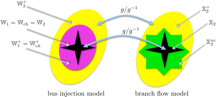
Figure 3: Feasible sets of conic formulations and their relaxations, and the relations among these sets. The sets $\mathbb{W}_{1}=\mathbb{W}_{ch}=\mathbb{W}_{2}$ on the left are the nonconvex feasible sets of equivalent OPF problems $\mathcal{P}_{1}$, $\mathcal{P}_{ch}$, $\mathcal{P}_{2}$ respectively in the bus injection model, and $\mathbb{W}_{1}^{+}=\mathbb{W}_{ch}^{+}\subseteq\mathbb{W}_{2}^{+}$ are the convex feasible sets of their respective relaxations $\mathcal{R}_{1},\mathcal{R}_{ch}$, $\mathcal{R}_{2}$. On the right, $\mathbb{X}_{2}$ is the nonconvex feasible set of an equivalent OPF problem $\tilde{\mathcal{P}}_{2}$ in the branch flow model. $\mathbb{X}_{2}^{nc}$ is the nonconex feasible set of the relaxation $\tilde{\mathcal{R}}_{2}^{nc}$ obtained by eliminating the voltage phase angles and $\mathbb{X}_{2}^{+}$ is the convex feasible set of the relaxation $\tilde{\mathcal{R}}_{2}$. The equivalence of the sets $\mathbb{W}_{2}$ (or $\mathbb{W}_{2}^{+}$) and $\mathbb{X}_{2}$ (or $\mathbb{X}_{2}^{+}$) is represented by the linear maps $g/g^{-1}$. When $G$ is a tree, $\mathbb{W}_{1}^{+}=\mathbb{W}_{ch}^{+}=\mathbb{W}_{2}^{+}$ in the bus injection model and $\mathbb{X}_{2}^{nc}=\mathbb{X}_{2}^{+}$ in the branch flow model. Note that neither of $\mathbb{W}_{1}^{+}$ and $\mathbb{X}_{2}^{nc}$ (or, more precisely $g^{-1}(\mathbb{X}_{2}^{nc})$ ) contains the other.

Proof:

We only prove part (a); part (b) follows similarly. Recall the definitions of sets $\mathbb{W}_{2}$ and $\mathbb{X}_{2}$:

$$\mathbb{W}_{2} :=\left\{W_{G}\ |\ W_{G}\text{ satisfies }\eqref{eq:opfW.1}-\eqref{eq:opfW.2}\text{ and }\eqref{eq:cyclecond},\right.$$

$$\qquad\qquad\left.{W_{G}}(e)\succeq 0,\ \operatorname{\text{rank}}{W_{G}}(e)=1\text{ for all $e\in E$}\right\},$$

$${\mathbb{X}}_{2} :=\{x\in\mathbb{R}^{n+3m}\ |\ x\text{ satisfies }(\ref{eq:bfm.1a}),\eqref{eq:opfB.2},\eqref{eq:Kirchhoff.2c},\eqref{eq:Kirchhoff.2d},\eqref{eq:cyclecond.2}\}.$$

We need to show that

1. $g(\mathbb{W}_{2})\subseteq\mathbb{X}_{2}$ so that $g:\mathbb{W}_{2}\rightarrow\mathbb{X}_{2}$ is well defined.

2. $g$ is injective, i.e., $g(x)\neq g(x^{\prime})$ if $x\neq x^{\prime}$.

3. $g$ is surjective and hence its inverse exists; moreover $g^{-1}$ defined in (28)–(29) is indeed $g$’s inverse.

The proof of (i) is similar to that of (iii) and omitted. That $g$ is injective follows directly from (25)–(27). To prove (iii), we need to show that given any $x:=(S,\ell,v)\in\mathbb{X}_{2}$, $W_{G}:=g^{-1}(x)$ defined by (28)–(29) is in $\mathbb{W}_{2}$ and $x=g(W_{G})$. We now prove this in four steps.

Step 1: Proof that $W_{G}$ satisfies (7a)–(7b). Clearly (7b) follows from (14). We now show that (7a) is equivalent to (13). For node $j\in N$, separate the edges in the summation in (7a) into outgoing edges $j\rightarrow k\in\tilde{E}$ from node $j$ and incoming edges $k\rightarrow j\in\tilde{E}$ to node $j$. For each incoming edge $k\rightarrow j\in\tilde{E}$ we have from (28)–(29)

$$[W_{G}]_{jj}-[W_{G}]_{jk} =v_{j}-\left(v_{k}-z_{kj}^{H}S_{kj}\right)^{H}$$

$$=-\left(v_{k}-v_{j}-z_{kj}S_{kj}^{H}\right)$$

$$=-\left(z_{kj}^{H}S_{kj}-|z_{kj}|^{2}\ell_{kj}\right),$$

where the last equality follows from (17). Substituting this and (28)–(29) into (7a) we get, for each $j\in N$:

$$\sum_{k:(j,k)\in E}\left([W_{G}]_{jj}-[W_{G}]_{jk}\right)y_{jk}^{H}$$

$$\qquad=\sum_{k:j\rightarrow k\in\tilde{E}}\left([W_{G}]_{jj}-[W_{G}]_{jk}\right)y_{jk}^{H}$$

$$\qquad\qquad+\sum_{k:k\rightarrow j\in\tilde{E}}\left([W_{G}]_{jj}-[W_{G}]_{jk}\right)y_{jk}^{H}$$

$$\qquad=\sum_{k:j\rightarrow k\in\tilde{E}}\left(v_{j}-(v_{j}-z_{jk}^{H}S_{jk})\right)y_{jk}^{H}$$

$$\qquad\qquad-\sum_{k:k\rightarrow j\in\tilde{E}}\left(z_{kj}^{H}S_{kj}-|z_{kj}|^{2}\ell_{kj}\right)y_{kj}^{H}$$

$$\qquad=\sum_{k:j\rightarrow k}S_{jk}\ -\sum_{k:k\rightarrow j}\left(S_{kj}-z_{kj}\ell_{kj}\right).$$

Hence, (7a) is equivalent to (13).

Step 2: Proof that $W_{G}$ satisfies (8). Without loss of generality let $c:=(1,2,\dots,k)$ be a cycle. For each directed edge $i\rightarrow j\in\tilde{E}$, recall $\beta_{ij}(x):=\angle(v_{i}-z_{ij}^{H}S_{ij})$ defined in (20) and define $\beta_{ji}(x)=-\beta_{ij}(x)$ in the opposite direction. Since $x=(S,\ell,v)$ satisfies (21), [37, Theorem 2] implies that

$$\beta_{12}(x)+\dots+\beta_{k1}(x) = 0\mod 2\pi,$$ (31)

where each $(i,j)$ in $c$ may be in the same or opposite orientation as the orientation of the directed graph $\tilde{G}$. Observe from (29) that, for each directed edge $i\rightarrow j\in\tilde{E}$, $\angle[W_{G}]_{ij}=\beta_{ij}(x)$ and $\angle[W_{G}]_{ji}=\beta_{ji}(x)$. Hence (31) is equivalent to (8), i.e., $\sum_{(i,j)\in c}\angle[W_{G}]_{ij}=0\mod 2\pi$.

Step 3: Proof that $W_{G}(e)\succeq 0,\operatorname{\text{rank}}{W_{G}}(e)=1$ for all $e\in E$. For each edge $i\rightarrow j\in\tilde{E}$ we have

$$[W_{G}]_{ii}[W_{G}]_{jj}-[W_{G}]_{ij}[W_{G}]_{ij}^{H}$$ (32)

$$\quad=v_{i}v_{j}-\left|v_{i}-z_{ij}^{H}S_{ij}\right|^{2}$$

$$\quad=v_{i}v_{j}-\left(v_{i}^{2}-v_{i}(z_{ij}S_{ij}^{H}+z_{ij}^{H}S_{ij})+|z_{ij}|^{2}|S_{ij}|^{2}\right)$$

$$\quad=-v_{i}\left(v_{i}-v_{j}-(z_{ij}S_{ij}^{H}+z_{ij}^{H}S_{ij})+|z_{ij}|^{2}\ell_{ij}\right),$$ (33)

where the last equality follows from (18). Substituting (17) into (33) yeilds $[W_{G}]_{ii}[W_{G}]_{jj}=\left|[W_{G}]_{ij}\right|^{2}$. This together with $[W_{G}]_{ii}\geq 0$ (from (28)) means $W_{G}(i,j)\succeq 0$ and $\operatorname{\text{rank}}{W_{G}}(i,j)=1$.

Step 4: Proof that $g(W_{G})=x$. Steps 1–3 show that $W_{G}:=g^{-1}(x)\in\mathbb{W}_{2}$ and hence $g$ has an inverse. We now prove this inverse is $g^{-1}$ defined by (28)–(29). It is easy to see that (25)–(26) follow directly from (28)–(29). We hence are left to show that $W_{G}$ satisfies (27). For each edge $i\rightarrow j\in\tilde{E}$ we have from (28)–(29)

$$|y_{ij}|^{2}\left([W_{G}]_{ii}+[W_{G}]_{jj}-[W_{G}]_{ij}-[W_{G}]_{ji}\right)$$

$$\quad=|y_{ij}|^{2}\left(v_{i}+v_{j}-2\,\text{Re }(v_{i}-z_{ij}^{H}S_{ij})\right)$$

$$\quad=|y_{ij}|^{2}\left(v_{j}-v_{i}+2\,\text{Re }(z_{ij}^{H}S_{ij})\right)$$

$$\quad=\ell_{ij},$$

where the last equality follows from (17). Hence $W_{G}$ satisfies (27) and $g(W_{G})=x$. ∎

We end this section with a visualization of Theorems 1, 5 and 6 in Figure 3. For any chordal extension $G_{ch}$ of graph $G$, the bus-injection model leads to three sets of problems $\mathcal{P}_{1},\mathcal{P}_{ch}$, and $\mathcal{P}_{2}$ and their corresponding relaxations $\mathcal{R}_{1},\mathcal{R}_{ch}$ and $\mathcal{R}_{2}$ respectively. The branch flow model leads to an equivalent OPF problem $\tilde{\mathcal{P}}_{2}$, a nonconvex relaxation $\tilde{\mathcal{R}}_{2}^{nc}$ obtained by eliminating the voltage phase angles, and its convex relaxation $\tilde{\mathcal{R}}_{2}$. The feasible sets of these problems, their relations, and the equivalence of the two models are explained in the caption of Figure 3.

V Numerics

We now illustrate the theory developed so far through simulations. First we visualize in Section V-A the feasible sets of OPF and their relaxations for a simple 3-bus example from [51]. Next we report in Section V-B the running times and accuracies (in terms of exactness) of different relaxations on IEEE benchmark systems.

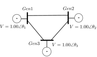
Figure 4: A 3-bus network from [51].

Parameter	Value
$y_{11}$	i0.3750
$y_{22}$	i0.5
$y_{33}$	i0.5750
$y_{12}$	0.0517 - i1.1087
$y_{13}$	0.1673 - i1.5954
$y_{23}$	0.0444 - i1.3319

TABLE I: Admittances for the 3-bus network.

V-A A 3-bus example

Consider the 3-bus example in Figure 4 taken from [51] (but we do not impose line limits) with line parameters in per units in Table I. Note that this network has shunt elements. For this example, $\mathcal{P}_{1}$ is the same problem as $\mathcal{P}_{ch}$ and $\mathcal{R}_{1}$ is the same problem as $\mathcal{R}_{ch}$. Hence we will focus on the feasible sets of $\mathcal{P}_{1}$ (which is the same as that of $\mathcal{P}_{2}$) and the feasible sets of $\mathcal{R}_{1}$, $\mathcal{R}_{2}$. Each problem has a Hermitian $3\times 3$ matrix $W$ as its variable. Recall that $s_{j}=p_{j}+\textbf{i}q_{j}$ is the complex power injection at node $j\in N$ and thus for each Hermitian matrix $W$, we have the following map:

$$p_{j}(W)+\textbf{i}q_{j}(W)=W_{jj}\ y_{jj}+\sum_{k:(j,k)\in E}\left(W_{jj}-W_{jk}\right)y_{jk}^{H}.$$

To visualize the various feasible sets, define the following set in 2 dimensions:

$$\mathcal{A}_{1} :=\left\{\left(p_{1}(W),p_{2}(W)\right)\ |\ W\in\mathbb{W}_{1},\right.$$

$$\qquad\quad\left.W_{11}=W_{22}=W_{33}=1,p_{3}(W)=-0.95\right\}.$$ (34)

This is the projection of the feasible set of $\mathcal{P}_{1}$ on the $p_{1}-p_{2}$ plane. Similarly, define the sets $\mathcal{A}_{1}^{+}$ and $\mathcal{A}_{2}^{+}$ where the Hermitian matrix $W$ is restricted to be in $\mathbb{W}_{1}^{+}$ and $\mathbb{W}_{2}^{+}$, respectively. We plot $\mathcal{A}_{1}$, $\mathcal{A}_{1}^{+}$ and $\mathcal{A}_{2}^{+}$ in Figure 5. It illustrates the relationship among the sets in Figure 3, i.e., $\mathbb{W}_{1}\subseteq\mathbb{W}_{1}^{+}\subseteq\mathbb{W}_{2}^{+}$. From Figure 5, $\mathcal{A}_{1}$ is non-convex while $\mathcal{A}_{1}^{+}$ and $\mathcal{A}_{2}^{+}$ are convex. Since $W\to(p_{1}(W),p_{2}(W))$ is a linear map, this confirms that $\mathbb{W}_{1}$ is non-convex while $\mathbb{W}_{1}^{+}$ and $\mathbb{W}_{2}^{+}$ are convex. To investigate the exactness of relaxations, consider the Pareto fronts of the various sets (magnified in Figure 5). The Pareto front of $\mathcal{A}_{1}^{+}$ coincides with that of $\mathcal{A}_{1}$ and thus relaxation $\mathcal{R}_{1}$ is exact; relaxation $\mathcal{R}_{2}$, however, is not.

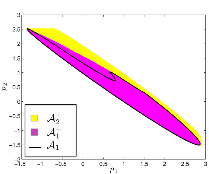
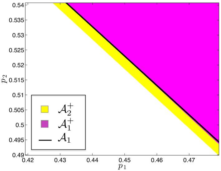
Figure 5: (a) Projections of feasible regions on $p_{1}-p_{2}$ space for the 3-bus system in Figure 4.
(b) Zoomed-in Pareto fronts of these sets.

Consider the set $\mathbb{W}_{2}^{nc}$ defined in (30) that is equivalent to $\mathbb{X}_{2}^{nc}$. For this example, $\mathbb{W}_{2}^{nc}$ is the set of $3\times 3$ matrices $W$ that satisfy (7a)-(7b) and the submatrices $W(1,2),W(2,3),W(1,3)$ are psd rank-1. The full matrix $W$, however, may not be psd or rank-1. Extend the definition of $\mathcal{A}_{1}$ in (34) to define the set $\mathcal{A}_{2}^{nc}$ where the matrix $W$ is restricted to be in $\mathbb{W}_{2}^{nc}$. In Figure 7, we plot $\mathcal{A}_{2}^{nc}$ along with $\mathcal{A}_{2}^{+}$ and $\mathcal{A}$. This equivalently illustrates the relation of the sets on the right in Figure 3.

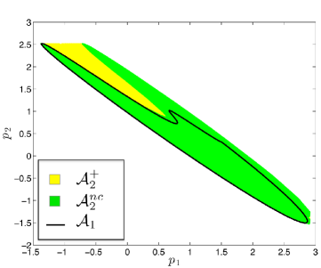
Figure 6: Projections of feasible regions on $p_{1}-p_{2}$ space for the 3-bus system in Figure 4.

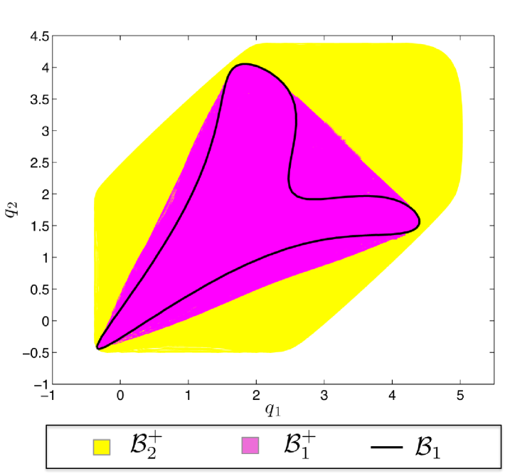
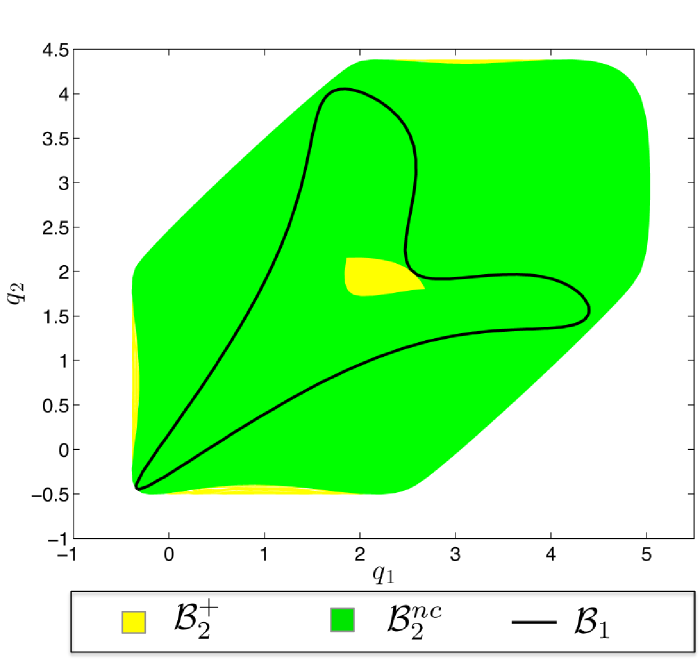
Figure 7: Projections of feasible regions on $q_{1}-q_{2}$ space for 3-bus system in Figure 4.

For the projections on the $q_{1}-q_{2}$ plane define the set

$$\mathcal{B}_{1} :=\left\{\left(q_{1}(W),q_{2}(W)\right)\ |\ W\in\mathbb{W}_{1},\right.$$

$$\qquad\quad\left.W_{11}=W_{22}=W_{33}=1,\ p_{3}(W)=-0.95\right\}.$$

As before, extend the definitions to $\mathcal{B}_{1}^{+}$, $\mathcal{B}_{2}^{+}$, and $\mathcal{B}_{2}^{nc}$. We plot $\mathcal{B}_{1}$, $\mathcal{B}_{1}^{+}$ and $\mathcal{B}_{2}^{+}$ in Figure 7 and $\mathcal{B}_{1}$, $\mathcal{B}_{2}^{nc}$ and $\mathcal{B}_{2}^{+}$ in Figure 7. This plot illustrates that the set $\mathbb{W}_{2}^{nc}$ is not simply connected (a set is said to be simply connected if any 2 paths from one point to another can be continuously transformed, staying within the set). Note that neither of $\mathcal{B}_{1}^{+}$ and $\mathcal{B}_{2}^{nc}$ contains the other.

Test case	Objective value		Running times			Lambda ratio
	$R_{1},R_{ch}$	$R_{2}$	$R_{1}$	$R_{ch}$	$R_{2}$
9 bus	5297.4	5297.4	0.2	0.2	0.2	$1.15\times 10^{-9}$
14 bus	8081.7	8075.3	0.2	0.2	0.2	$8.69\times 10^{-9}$
30 bus	574.5	573.6	0.4	0.3	0.3	$1.67\times 10^{-9}$
39 bus	41889.1	41881.5	0.7	0.3	0.3	$1.02\times 10^{-10}$
57 bus	41738.3	41712.0	1.3	0.5	0.3	$3.98\times 10^{-9}$
118 bus	129668.6	129372.4	6.9	0.7	0.6	$2.16\times 10^{-10}$
300 bus	720031.0	719006.5	109.4	2.9	1.8	$1.26\times 10^{-4}$
2383wp bus	1840270	1789500.0	-	1005.6	155.3	median = $3.33\times 10^{-5}$, max =$0.0034$.

TABLE II: Performance comparison of relaxation techniques for IEEE benchmark systems.

V-B IEEE benchmark systems

For IEEE benchmark systems [52, 53], we solve $\mathcal{R}_{1}$, $\mathcal{R}_{2}$ and $\mathcal{R}_{ch}$ in MATLAB using CVX [68] with the solver SeDuMi [69] after some minor modifications to the resistances on some lines [23]. The objective values and running times are presented in Table II. The problems $\mathcal{R}_{1}$ and $\mathcal{R}_{ch}$ have the same optimal objective value, i.e., $r_{1}^{*}=r_{ch}^{*}$, as predicted by Theorem 1. We also report the ratios of the first two eigenvalues of the optimal $W^{*}$ in $\mathcal{R}_{1}$; for most cases, it is small indicating that the relaxation is exact. The optimal objective value of $\mathcal{R}_{2}$ is lower ($r_{2}^{*}<r_{1}^{*}$), indicating that the optimum of the SOCP relaxation that is computed is not feasible for $\mathcal{P}_{1}$. As Table II shows, $\mathcal{R}_{ch}$ is much faster than $\mathcal{R}_{1}$ for large networks. The chordal extensions of the graphs are computed a priori for each case [41]. $\mathcal{R}_{2}$ is faster than both $\mathcal{R}_{1}$ and $\mathcal{R}_{ch}$, but yields an infeasible solution for most IEEE benchmark systems considered.

VI Conclusion

In this paper, we have presented various conic relaxations of the OPF problem and their relations in both the bus injection and the branch flow models. In the bus injection model the SDP relaxations $\mathcal{R}_{1}$ and $\mathcal{R}_{ch}$ are equivalent and are generally tighter than the SOCP relaxation $\mathcal{R}_{2}$. For acyclic networks however these relaxations are equivalent. The branch flow model leads to an SOCP relaxation $\tilde{\mathcal{R}}_{2}$. We have shown that $\mathcal{R}_{2}$ and $\tilde{\mathcal{R}}_{2}$ are equivalent. In general $\mathcal{R}_{ch}$ is faster to compute than $\mathcal{R}_{1}$. $\mathcal{R}_{2}$ and $\tilde{\mathcal{R}}_{2}$ are even faster, though their feasible sets are generally larger than that of $\mathcal{R}_{1}$ or $\mathcal{R}_{ch}$.

References

- [1] Subhonmesh Bose, Steven H. Low, and Mani Chandy. Equivalence of branch flow and bus injection models. In 50th Annual Allerton Conference on Communication, Control, and Computing, October 2012.
- [2] J. Carpentier. Contribution to the economic dispatch problem. Bulletin de la Societe Francoise des Electriciens, 3(8):431–447, 1962. In French.
- [3] H.W. Dommel and W.F. Tinney. Optimal power flow solutions. Power Apparatus and Systems, IEEE Transactions on, PAS-87(10):1866–1876, Oct. 1968.
- [4] J. A. Momoh. Electric Power System Applications of Optimization. Power Engineering. Markel Dekker Inc.: New York, USA, 2001.
- [5] M. Huneault and F. D. Galiana. A survey of the optimal power flow literature. IEEE Trans. on Power Systems, 6(2):762–770, 1991.
- [6] J. A. Momoh, M. E. El-Hawary, and R. Adapa. A review of selected optimal power flow literature to 1993. Part I: Nonlinear and quadratic programming approaches. IEEE Trans. on Power Systems, 14(1):96–104, 1999.
- [7] J. A. Momoh, M. E. El-Hawary, and R. Adapa. A review of selected optimal power flow literature to 1993. Part II: Newton, linear programming and interior point methods. IEEE Trans. on Power Systems, 14(1):105 – 111, 1999.
- [8] K. S. Pandya and S. K. Joshi. A survey of optimal power flow methods. J. of Theoretical and Applied Information Technology, 4(5):450–458, 2008.
- [9] Stephen Frank, Ingrida Steponavice, and Steffen Rebennack. Optimal power flow: a bibliographic survey, I: formulations and deterministic methods. Energy Systems, 3:221–258, September 2012.
- [10] Stephen Frank, Ingrida Steponavice, and Steffen Rebennack. Optimal power flow: a bibliographic survey, II: nondeterministic and hybrid methods. Energy Systems, 3:259–289, September 2013.
- [11] Mary B. Cain, Richard P. O’Neill, and Anya Castillo. History of optimal power flow and formulations (OPF Paper 1). Technical report, US FERC, December 2012.
- [12] Richard P. O’Neill, Anya Castillo, and Mary B. Cain. The IV formulation and linear approximations of the AC optimal power flow problem (OPF Paper 2). Technical report, US FERC, December 2012.
- [13] Richard P. O’Neill, Anya Castillo, and Mary B. Cain. The computational testing of AC optimal power flow using the current voltage formulations (OPF Paper 3). Technical report, US FERC, December 2012.
- [14] Anya Castillo and Richard P. O’Neill. Survey of approaches to solving the ACOPF (OPF Paper 4). Technical report, US FERC, March 2013.
- [15] Anya Castillo and Richard P. O’Neill. Computational performance of solution techniques applied to the ACOPF (OPF Paper 5). Technical report, US FERC, March 2013.
- [16] S. H. Low. Convex relaxation of optimal power flow: a tutorial. In IREP Symposium – Bulk Power System Dynamics and Control (IREP), Rethymnon, Greece, August 2013.
- [17] B Stott and O. Alsaç. Fast decoupled load flow. IEEE Trans. on Power Apparatus and Systems, PAS-93(3):859–869, 1974.
- [18] O. Alsaç, J Bright, M Prais, and B Stott. Further developments in LP-based optimal power flow. IEEE Trans. on Power Systems, 5(3):697–711, 1990.
- [19] K. Purchala, L. Meeus, D. Van Dommelen, and R. Belmans. Usefulness of DC power flow for active power flow analysis. In Proc. of IEEE PES General Meeting, pages 2457–2462. IEEE, 2005.
- [20] B. Stott, J. Jardim, and O. Alsaç. DC Power Flow Revisited. IEEE Trans. on Power Systems, 24(3):1290–1300, Aug 2009.
- [21] Carleton Coffrin and Pascal Van Hentenryck. A linear-programming approximation of AC power flows. CoRR, abs/1206.3614, 2012.
- [22] X. Bai, H. Wei, K. Fujisawa, and Y. Wang. Semidefinite programming for optimal power flow problems. Int’l J. of Electrical Power & Energy Systems, 30(6-7):383–392, 2008.
- [23] J. Lavaei and S. H. Low. Zero duality gap in optimal power flow problem. IEEE Trans. on Power Systems, 27(1):92–107, February 2012.
- [24] S. Bose, D. Gayme, S. H. Low, and K. M. Chandy. Optimal power flow over tree networks. In Proc. Allerton Conf. on Comm., Ctrl. and Computing, October 2011.
- [25] B. Zhang and D. Tse. Geometry of feasible injection region of power networks. In Proc. Allerton Conf. on Comm., Ctrl. and Computing, October 2011.
- [26] S. Sojoudi and J. Lavaei. Physics of power networks makes hard optimization problems easy to solve. In IEEE Power & Energy Society (PES) General Meeting, July 2012.
- [27] Javad Lavaei, Anders Rantzer, and Steven H. Low. Power flow optimization using positive quadratic programming. In Proceedings of IFAC World Congress, 2011.
- [28] Lingwen Gan and Steven H. Low. Optimal power flow in DC networks. In 52nd IEEE Conference on Decision and Control, December 2013.
- [29] M. E. Baran and F. F Wu. Optimal Capacitor Placement on radial distribution systems. IEEE Trans. Power Delivery, 4(1):725–734, 1989.
- [30] M. E Baran and F. F Wu. Optimal Sizing of Capacitors Placed on A Radial Distribution System. IEEE Trans. Power Delivery, 4(1):735–743, 1989.
- [31] R. Cespedes. New method for the analysis of distribution networks. IEEE Trans. Power Del., 5(1):391–396, January 1990.
- [32] A. G. Expósito and E. R. Ramos. Reliable load flow technique for radial distribution networks. IEEE Trans. Power Syst., 14(13):1063–1069, August 1999.
- [33] R.A. Jabr. Radial Distribution Load Flow Using Conic Programming. IEEE Trans. on Power Systems, 21(3):1458–1459, Aug 2006.
- [34] Masoud Farivar, Christopher R. Clarke, Steven H. Low, and K. Mani Chandy. Inverter VAR control for distribution systems with renewables. In Proceedings of IEEE SmartGridComm Conference, October 2011.
- [35] Joshua A. Taylor and Franz S. Hover. Convex models of distribution system reconfiguration. IEEE Trans. Power Systems, 2012.
- [36] R. A. Jabr. Exploiting sparsity in sdp relaxations of the opf problem. Power Systems, IEEE Transactions on, 27(2):1138–1139, 2012.
- [37] Masoud Farivar and Steven H. Low. Branch flow model: relaxations and convexification (parts I, II). IEEE Trans. on Power Systems, 28(3):2554–2572, August 2013.
- [38] Lingwen Gan, Na Li, Ufuk Topcu, and Steven H. Low. On the exactness of convex relaxation for optimal power flow in tree networks. In Prof. 51st IEEE Conference on Decision and Control, December 2012.
- [39] Na Li, Lijun Chen, and Steven Low. Exact convex relaxation of opf for radial networks using branch flow models. In IEEE International Conference on Smart Grid Communications, November 2012.
- [40] Mituhiro Fukuda, Masakazu Kojima, Kazuo Murota, and Kazuhide Nakata. Exploiting sparsity in semidefinite programming via matrix completion I: General framework. SIAM Journal on Optimization, 11:647–674, 1999.
- [41] Etienne de Klerk. Exploiting special structure in semidefinite programming: A survey of theory and applications. European Journal of Operational Research, 201(1):1–10, 2010.
- [42] Miguel Soma Lobo, Lieven Vandenberghe, Stephen Boyd, and Hervé Lebret. Applications of second-order cone programming. Linear Algebra and its Applications, 284:193–228, 1998.
- [43] S. P. Boyd and L. Vandenberghe. Convex optimization. Cambridge University Press, 2004.
- [44] X. Bai and H. Wei. A semidefinite programming method with graph partitioning technique for optimal power flow problems. Int’l J. of Electrical Power & Energy Systems, 33(7):1309–1314, 2011.
- [45] S. Bose, D. Gayme, K. M. Chandy, and S. H. Low. Quadratically constrained quadratic programs on acyclic graphs with application to power flow. arXiv:1203.5599v1, March 2012.
- [46] W. H. Kersting. Distribution systems modeling and analysis. CRC, 2002.
- [47] D. Shirmohammadi, H. W. Hong, A. Semlyen, and G. X. Luo. A compensation-based power flow method for weakly meshed distribution and transmission networks. IEEE Transactions on Power Systems, 3(2):753–762, May 1988.
- [48] H-D. Chiang and M. E. Baran. On the existence and uniqueness of load flow solution for radial distribution power networks. IEEE Trans. Circuits and Systems, 37(3):410–416, March 1990.
- [49] Lingwen Gan, Na Li, Ufuk Topcu, and Steven H. Low. Optimal power flow in distribution networks. In Proc. 52nd IEEE Conference on Decision and Control, December 2013. in arXiv:12084076.
- [50] Lingwen Gan, Na Li, Ufuk Topcu, and Steven H. Low. Exact convex relaxation of optimal power flow in tree networks. submitted for publication, 2013.
- [51] B. Lesieutre, D. Molzahn, A. Borden, and C. L. DeMarco. Examining the limits of the application of semidefinite programming to power flow problems. In Proc. Allerton Conference, 2011.
- [52] University of Washington. Power systems test case archive.
- [53] R. D. Zimmerman, C. E. Murillo-Sánchez, and R. J. Thomas. MATPOWER’s extensible optimal power flow architecture. In Proc. IEEE PES General Meeting, pages 1–7, 2009.
- [54] A. R. Bergen and V. Vittal. Power Systems Analysis. Prentice Hall, 2nd edition, 2000.
- [55] R.A. Horn and C.R. Johnson. Matrix analysis. Cambridge university press, 2005.
- [56] H. Wolkowicz, R. Saigal, and L. Vandenberghe. Handbook of semidefinite programming: theory, algorithms, and applications, volume 27. Springer Netherlands, 2000.
- [57] Y. Nesterov and A. Nemirovskii. Interior-point polynomial algorithms in convex programming, volume 13. Society for Industrial Mathematics, 1987.
- [58] Farid Alizadeh. Interior point methods in semidefinite programming with applications to combinatorial optimization. SIAM Journal on Optimization, 5(1):13–51, 1995.
- [59] Baosen Zhang and David Tse. Geometry of the injection region of power networks. IEEE Trans. Power Systems, 28(2):788–797, 2013.
- [60] Javad Lavaei, David Tse, and Baosen Zhang. Geometry of power flows and optimization in distribution networks. arXiv, November 2012.
- [61] Albert Y.S. Lam, Baosen Zhang, Alejandro Domínguez-García, and David Tse. Optimal distributed voltage regulation in power distribution networks. arXiv, April 2012.
- [62] Somayeh Sojoudi and Javad Lavaei. Semidefinite relaxation for nonlinear optimization over graphs with application to power systems. Preprint, 2013.
- [63] D. R. Fulkerson and O. A. Gross. Incidence matrices and interval graphs. Pacific Journal of Mathematics, 15(3):835–855, 1965.
- [64] Donald J. Rose, Robert Endre Tarjan, and George S. Lueker. Algorithmic aspects of vertex elimination on graphs. SIAM Journal on Computing, 5(2):266–283, 1976.
- [65] Norman Biggs. Algebraic graph theory. Cambridge University Press, 1993. Cambridge Mathematical Library.
- [66] R. Grone, C. R. Johnson, E. M. Sá, and H. Wolkowicz. Positive definite completions of partial Hermitian matrices. Linear Algebra and its Applications, 58:109–124, 1984.
- [67] Takashi Tsuchiya. A polynomial primal-dual path-following algorithm for second-order cone programming. Research Memorandum, 649, 1997.
- [68] Michael Grant and Stephen Boyd. CVX: Matlab software for disciplined convex programming, version 2.0 beta. http://cvxr.com/cvx, September 2012.
- [69] Jos F. Sturm. Using SeDuMi 1.02, a MATLAB toolbox for optimization over symmetric cones. Optimization Methods and Software, 11:625–653, 1999.