Robust Large-Scale Non-Negative Matrix Factorization Using Proximal Point Algorithm
Abstract
A robust algorithm for non-negative matrix factorization (NMF) is presented in this paper with the purpose of dealing with large-scale data, where the separability assumption is satisfied. In particular, we modify the Linear Programming (LP) algorithm of [9] by introducing a reduced set of constraints for exact NMF. In contrast to the previous approaches, the proposed algorithm does not require the knowledge of factorization rank (extreme rays[3] or topics [7]). Furthermore, motivated by a similar problem arising in the context of metabolic network analysis[13], we consider an entirely different regime where the number of extreme rays or topics can be much larger than the dimension of the data vectors. The performance of the algorithm for different synthetic data sets are provided.
I Introduction
Matrix factorization has numerous applications to the real-world problems where the data matrices representing the numerical observations are often huge and hard to analyze. Meanwhile, factorizing them into lower-rank forms is able to reveal the inherent structure and features, which helps in the meaningful interpretation of the data. In a wide range of natural signals, such as pixel intensities, amplitude spectra, and occurance counts, negative values are usually physically meaningless. In order to deal with this non-negative constraint, Non-Negative Matrix Factorization (NMF) was introduced.
NMF was first proposed in [1] and used by Lee and Seung for parts-based data representation [2]. It is well known that NMF may not be unique. In this context a sufficient condition on the uniqueness of NMF was pointed out in [3]. A geometrical interpretation [4], of this condition amounts to the fact that the extreme rays (topics) generating the cone (in the non-negative orthant) are contained in the data. Thus, for NMF, one only needs to identify these extreme rays. Additionally, it was demonstrated in [5] that under such a separability assumption, one can use Linear Programming (LP) to isolate the extreme rays from the non-extreme rays. In this paper we will focus only on such cases.
Bittorf et al.[9] presented a LP-based NMF algorithm named Hottopixx. Kumar et al.[4], instead, presented a fast conical hull algorithm to deal with the large-scale NMF based on its polyhedral structure. It was shown to perform much faster than Hottopixx. However, both of these algorithms require the factorization rank, i.e. the number of extreme rays as a necessary input. Some applications will grant this as prior knowledge but from the view of robustness, the preference would go to a robust NMF algorithm. Gillis and Luce [10] reformulated the algorithm in [9] to detect the number of extreme rays automatically. Nevertheless, the limitation still exists with the fact that the number of constraints in the LP is enormous in face of the large-scale data.
Alternatively, motivated by Theorem 5.4 in[5], we propose a simpler modification of the constraints to alleviate these issues. In particular we reduce the number of constraints and do not require that the number of extreme rays to be known. This allows us to use a proximal point-based algorithm [12] to solve the LP problem efficiently for data sets with large size.
In addition we also consider an entirely different regime from the NMF applications in the literature so far, where the data lies high dimension with a much smaller factorization rank (the number of extreme rays) in comparison. Specifically, we look at the case when the number of extreme rays is much larger than the dimensionality of the space. This is caused by the computational issues, which arises in Double Description (DD) method [6] for the analysis of metabolic networks to find the Elementary Flux Modes (EFMs) as the set of extreme rays of the polyhedral cone [13]. A NMF like problem arises as an intermediate step in DD method. In this context, we believe that the computational advances in NMF can help with addressing the computational issues in the DD method [6].
The organization of the paper is as follows. Section II provides a brief review of NMF from the geometric perspective as well as the Hottopixx algorithm. Section III explains the proposed proximal point algorithm with the reformulated LP constraints. The experiments results are presented in Section IV and the paper concludes in Section V.
Notation: The matrices will be denoted by boldface capital letters and vectors by boldface small letters. In addition we use the MATLAB notation of diag to transform vectors to diagonal matrices and to extract the diagonal from the matrix in the argument. Also we use the MATLAB and the operators for matrix concatenations.
II Non-negative Matrix Factorization
For the non-noisy case, given a data matrix . Therefore, NMF aims to find two nonnegative matrices and such that . For an approximate NMF, instead, the aim is to solve the following optimization problem.
| (1) |
II-A Geometry of the NMF Problem
The factorization implies that all the columns of can be represented as non-negative combination of the columns of the matrix . The algebraic characterization can be described as below.
Definition 1.
The generated by columns is given by,
| (2) |
The factorization refers geometrically to that the all lie in or on the surface of the simplical cone generated by the , as depicted in Fig. 1.
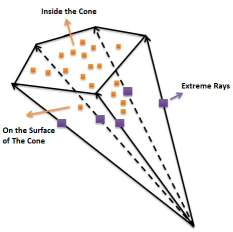
With this viewpoint in mind, we define three assumptions as follows.
-
•
Assumption 1: Extreme rays by definition are simplicial: No extreme ray is in the convex combination of the other extreme rays. This is also shown to be necessary and sufficient for exact recovery in topic modeling [8].
-
•
Assumption 2: The dataset consisting of all columns of , reside in or on the surface of a cone generated by these extreme rays of [3].
-
•
Assumption 3: Assuming that the columns of are normalized to unity there are no duplicate columns in .
The above three assumptions will be collectively referred to as separability assumption in the following: The entire dataset, i.e. all columns of , reside in or on a surface of a cone generated by a small subset of columns of , the vectors in this subset being simplicial and there are no duplicate columns in after column normalization.
In algebraic terms, for some subset of columns (extreme rays) of and where denotes the matrix built with columns of indexed by . This means that the vectors of are hidden among the columns of ( is unknown) [5]. Equivalently, it implies that the corresponding subset of rows of constitutes the weight matrix. Therefore, the computational challenge is to identify the extreme rays efficiently. In this context, we first outline the LP-based Hottopixx Algorithm from [9] .
II-B Hottopixx
Bittorf et al.[9] proposed an algorithm of NMF under separability assumption based on the following LP problem:
| (3) |
and is a random vector with distinct positive entries and is referred to as a factorization localizing matrix[9], which belongs to the following polyhedral set.
| (4) |
For a large scale set-up they proposed an incremental gradient descent algorithm to solve the LP.
III Robust NMF Using Proximal Point Algorithm
As explained before, two of the prominent shortcomings of existing algorithms for the NMF problem are - (i) Dependence on knowledge of the number of extreme rays and, (ii) Dealing with a large data set resulting in an enormous number of constraints. An approach in this direction was taken in [10]. However, the number of constraints in their reformulation is still immense for large data. In this paper we present a reformulation which drastically reduces the set of constraints.
III-A LP Reformulation
Assuming that the columns of are normalized to have an unit norm, our LP reformulation for NMF is given as
| (5) |
where,
| (6) |
where is the vector of all -s and is the same as the vector in (LABEL:eq2_2).
Proposition 1.
Suppose admits a separable factorization , compute the minimization of (5) and let , then .
In order to prove the above proposition, we consider the Lagrangian of the optimization problem in (5), which is,
| (7) | ||||
where and are the Lagrange multipliers. Then the dual form of (5) is
| (8) | ||||||
| s.j.t |
The proof of the proposition follows from Lemma 1 and Lemma 2 below.
Lemma 1.
If .
Proof.
For , consider the LP problem
| (9) |
where denotes the vector with th entry and the rest . Assign and using the constraint , we can claim that . Under the separability assumption, there exists a collection of vectors such that,
| (10) | |||||
for and some . A feasible solution to (LABEL:eq_9) is
| (11) | ||||
With such selection, the dual cost function is equal to . From weak duality [11] it follows that . Combined with , it implies and . ∎
Lemma 2.
If .
Proof.
For , Consider the LP problem
| (12) |
Note that the constraint implies that therefore . For the dual program a feasible solution can be found as
| (13) | ||||
for which the dual cost function (LABEL:eq_9) is equal to 1. Again using the weak duality [11], it implies that and from , we have and . ∎
Proof of Proposition 1.
Let denote the factorization localizing matrix which identifies the factorization with lowest cost and has either ones or zeros on the diagonal. Then is the unique optimal solution of (5). To see this, let denote the set of simplicial columns of minimum cost. Since each column of can only belong to or not, once is given, is determined then the lowest cost is determined, which is unique.
Remark.
Note that can be readily obtained from as (in MATLAB notation).
III-B Proximal Point Algorithm
Based on the above reformulation, a proximal point-based (Proximal Point) algorithm is employed in this paper. A necessary pre-processing step is the column normalization, which makes sure that the sum of each column of is equal to one.
We solve this LP using the proximal point algorithm [12] in Algorithm 1 and in our implementation, are set to a large constant . The discussion on the convergence of the algorithm can be found in [12].
Input: A column normalized matrix , stopping threshold .
Output: A matrix and , and .
IV Experiments Results
All of the experiments were run on an identical configuration: a dual Xeon W3505 (2.53GHz) machine with 6GB RAM. Proximal Point Algorithm is examined in MATLAB with the version of 2013a.
IV-A Random Data Generation
To generate our instances, independent extreme rays are firstly created in , with the element value between . The remaining columns are then generated to be the random non-negative combinations of the extreme rays, where is randomly selected for each of the points. The column normalization is carried out sequentially. Three regimes of NMF problems are analyzed here:
Furthermore, since the algorithm is free from the order of the columns, the extreme rays are allocated at the beginning of each data set.
Different size of data sets are generated to check the effectiveness of Proximal Point Algorithm, from small to large-scale. In Tab. I, the last column indicates the highest level for iteration stopping criterion to achieve the listed accuracy. From the experiments, it is exhibited that our algorithm can deal with three regimes of the data with different sizes. Moreover, the identification accuracy is satisfying.
| Data Set | # of Extreme Rays | Accuracy | |
|---|---|---|---|
| (C1) | 25 | ||
| (C1) | 25 | ||
| (C1) | 300 | ||
| (C2) | 15 | ||
| (C2) | 75 | ||
| (C2) | 225 | ||
| (C3) | 45 | ||
| (C3) | 150 | ||
| (C3) | 625 |
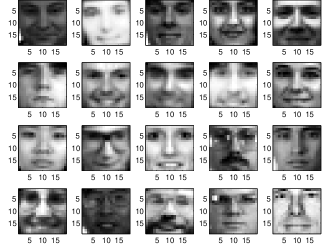
IV-B Application to Image Processing
In this section, we apply the Proximal Point algorithm to one face image processing data set, namely, CBCL Dataset[14]. Basically, the CBCL face dataset is made of 2429 gray-level face images with pixels. We randomly choose images from the dataset with vectorization to be the generators, which means the number of extreme rays in this case is . Through the random non-negative combination of the extreme rays, a facial data matrix is created. Applying Proximal Point algorithm to this dataset, the results of the extreme rays identification are shown in Fig. 2, which represents the initial images as generators.
V Acknowledgements
The second author would like to acknowledge several useful discussions with Prof. Prakash Ishwar at Boston University.
References
- [1] P. Paatero and U. Tapper, “Positive Matrix Factorization: A non-negative factor model with optimal utilization of error estimates of data values,” Environmetrics, vol. 5, pp. 111-126, 1994.
- [2] D. Lee and H. Seung,“Algorithms for Non-Negative Matrix Factorization,” in NIPS, 2001, pp. 556-562.
- [3] D. Donoho and V. Stodden, “When does non-negative matrix factorization give a correct decomposition into parts,” in NIPS, 2004, MIT Press.
- [4] A. Kumar, V. Sindhwani, and P. Kambadur, “Fast conical hull algorithms for near-separable non-negative matrix factorization,” arXiv:1210.1190, 2012.
- [5] S. Arora, R. Ge, R. Kannan, and A. Moitra, “Computing a nonnegative matrix factorization – provably,” in STOC, 2012, pp.145-162.
- [6] K. Fukuda and A. Prodon. “Double description method revisited.” in Combinatorics and Computer Science, vol. 1120, pp. 91-111, 1996.
- [7] W. Ding, M. H. Rohban, P. Ishwar, V. Saligrama, “A New Geometric approach to latent topic modeling and discovery,”arXiv:1301.0858 [stat.ML], 2013.
- [8] W. Ding, P. Ishwar, M. H. Rohban, V. Saligrama, “Necessary and Sufficient Conditions for Novel Word Detection in Separable Topic Models,” arXiv:1310.7994 [cs.LG], 2013.
- [9] B. Recht, C. Re, J. Tropp, and V. Bittorf, “Factoring nonnegative matrices with linear programs,” in NIPS,2012, pp. 1223-1231.
- [10] N. Gillis and R. Luce, “Robust near-Separable nonnegative matrix factorization using linear optimization,” arXiv:1302.4385, 2013.
- [11] D.G. Luenberger, Optimization by vector space methods. New York: Wiley, 1969.
- [12] J. Ekstein, “Nonlinear proximal point algorithms using Bregman functions with applications to convex programming,” Math. Oper. Res., vol. 18, pp. 203-226, 1993.
- [13] M. Terzer and J. Stelling, “Accelerating the Computation of Elementary Modes Using Pattern Trees,” in WABI, 2006, pp. 333-343.
- [14] http://cbcl.mit.edu/software-datasets/FaceData2.html
- [15] D. P. Bertsekas, “A new class of incremental gradient methods for least squares problems,” SIAM J. Optim., vol. 7, no. 4, pp. 913-926, 1997.