Neutrino masses in RPV models with
two pairs of Higgs doublets

Yuval Grossman¹ and Clara Peset ²

¹Laboratory for Elementary-Particle Physics, Cornell University, Ithaca, N.Y.

²IFAE, Universitat Autònoma de Barcelona, 08193 Bellaterra, Barcelona

We study the generation of neutrino masses and mixing in supersymmetric R-parity violating models containing two pairs of Higgs doublets. In these models, new RPV terms $\hat{H}_{D_{1}}\hat{H}_{D_{2}}\hat{E}$ arise in the superpotential, as well as new soft terms. Such terms give new contributions to neutrino masses. We identify the different parameters and suppression/enhancement factors that control each of these contributions. At tree level, just like in the MSSM, only one neutrino acquires a mass due to neutrino-neutralino mixing. There are no new one loop effects. We study the two loop contributions and find the conditions under which they can be important.

1 Introduction

Neutrinos have a non-zero mass matrix, as is indicated by neutrino oscillation experiments. This fact requires some extension of the Standrad Model (SM) that incorporates both their masses and their mixing angles [1, 2, 3]. The experimental data [4],

$$\leavevmode\nobreak\ \leavevmode\nobreak\ \leavevmode\nobreak\ \leavevmode\nobreak\ \leavevmode\nobreak\ \leavevmode\nobreak\ \Delta m_{32}^{2}=\left(2.32^{+0.12}_{-0.08}\right)\times 10^{-3}\,\mathrm{eV}^{2},\qquad\Delta m_{21}^{2}=(7.5\pm 0.20)\times 10^{-5}\,\mathrm{eV}^{2},$$ (1)

$$\sin^{2}(2\theta_{32})>0.95,\qquad\sin^{2}(2\theta_{12})=0.857\pm 0.024,\qquad\sin^{2}(2\theta_{13})=0.095\pm 0.010,$$

exhibit a mild mass hierarchy, two large mixing angles, and one mixing angle that is somewhat smaller. This structure poses a challenge for new physics where, generally, mass hierarchies come with small mixing angles. This is solved when different neutrinos obtain their masses from different sources. Then, cancellations in the determinant of the mass matrix can arise naturally, making its value smaller than the typical values of the elements of the matrix. Neutrinos in R-Parity Violating (RPV) supersymmetric models have been widely studied [5] and have been shown to be a framework in which this property is accomplished. In these models one neutrino acquires a mass at tree level through neutrino-neutralino mixing, while the other two acquire their masses from loop effects.

Models with extra Higgs doublets have been widely studied both in the context of the SM [6] and supersymmetry (SUSY) [7]. In the SUSY case, the simplest way to ensure anomaly cancellation is to add pairs of down-type and up-type Higgs fields. Lately, such models have been proposed as a way of naturally lifting the mass of the lightest Higgs boson, which in the Minimal Supersymmetric Model (MSSM) cannot be $125\,\mathrm{GeV}$ without some amount of fine tuning [8]. When R-parity is not imposed in these models, new renormalizable terms of the form $\hat{H}_{D_{i}}\hat{H}_{D_{j}}\hat{E}$ arise in the superpotential. Such new terms can substantially contribute to the neutrino mass matrix since their couplings are less constrained than the conventional leptonic RPV couplings.

In this work we study how neutrino masses arise in a general supersymmetric model with more than the minimal number of Higgs doublets. The large number of free parameters in the model does not allow to make predictions without any kind of further assumption. Nevertheless, we identify the suppression and enhancement factors in the various contributions to the neutrino mass matrix. We find that, even with two pairs of Higgs doublets, only one neutrino acquires a mass at tree level, just like in the MSSM. We describe the loop diagrams generated by the new RPV terms in the superpotential, which arise at the two loop level, and in the appendix we give expressions for the relevant one loop diagrams within our model. We study which of these diagrams may give relevant contributions to the neutrino masses.

One major issue in models with several Higgs doublets is that generally they generate flavor changing neutral currents (FCNCs) that can cause severe phenomenological problems. There are several ways to avoid such bounds, for example by assuming a specific texture for the Yukawa couplings to the quark sector, or by assuming Minimal Flavor Violation (MFV), see, for example [6]. In this work we only concentrate on the leptonic sector and thus we do not elaborate on the quark sector, and just assume that one of the available solutions to the FCNCs bounds is in place.

2 The model

We work with a general RPV low-energy supersymmetric model with one extra pair of Higgs doublets, namely, we consider two up-type and two down-type Higgs doublets. We follow the notation of [9] where the model with just one pair of Higgs doublets is fully described. Neutrino masses arise from diagrams which violate lepton number by two units. In order to avoid the bounds from proton stability, we choose only terms which still preserve ${\bf Z_{3}}$ baryon triality [10]. When R-parity is not imposed, the down-type Higgs supermultiplets $\hat{H}_{D_{1}}$ and $\hat{H}_{D_{2}}$ have the same quantum numbers as the lepton supermultiplets $\hat{L}_{i}$. We denote the five supermultiplets by one only symbol $\hat{L}_{I}$ ($I=0,1,2,3,4$) such that $\hat{L}_{0}\equiv\hat{H}_{D_{1}}$, $\hat{L}_{1}\equiv\hat{H}_{D_{2}}$ and $\hat{L}_{1+i}\equiv\hat{L}_{i}$. Throughout this work we will use the following index notation: upper-case Latin letters for the extended five-dimensional lepton flavor space, Greek letters for four-dimensional flavor spaces and lower-case Latin letters for three-dimensional ones.

The relevant renormalizable superpotential for this model is

$$W = \epsilon_{ij}\left[-\mu_{1I}\hat{L}_{I}^{i}\hat{H}_{U_{1}}^{j}-\mu_{2I}\hat{L}_{I}^{i}\hat{H}_{U_{2}}^{j}+\frac{1}{2}\lambda_{IJm}\hat{L}_{I}^{i}\hat{L}_{J}^{j}\hat{E}_{m}+\lambda^{\prime}_{Inm}\hat{L}_{I}^{i}\hat{Q}_{n}^{j}\hat{D}_{m}\right],$$ (2)

where $\hat{H}_{U_{i}}\ ,i=1,2$, are the two up-type Higgs supermultiplets, $\hat{Q}_{n}$ are the quark doublet supermultiplets, $\hat{U}_{m}$ ($\hat{D}_{m}$) are the up-type (down-type) quark supermultiplets, and $\hat{E}_{m}$ are the singlet charged lepton supermultiplets. The $n$ and $m$ are flavor indices. The coefficients $\lambda_{IJm}$ are antisymmetric under the exchange of the indices $I$ and $J$. The usual MSSM $\mu$-term is now extended to two five-dimensional vectors, $\mu_{1I}$ and $\mu_{2I}$. Note that, in comparison with the RPV models already studied in [11, 12, 13], a new type of trilinear $\lambda$-term arises for the two down-type Higgs supermultiplets, which is less constrained than the conventional leptonic RPV terms,

$$\frac{\tilde{\lambda}_{m}}{2}\epsilon_{ij}\left(\hat{H}_{D_{1}}^{i}\hat{H}_{D_{2}}^{j}-\hat{H}_{D_{2}}^{i}\hat{H}_{D_{1}}^{j}\right)\hat{E}_{m},$$ (3)

where $\tilde{\lambda}_{m}=\lambda_{01m}$.

In order to compute all the contributions to the neutrino masses we need to consider the following soft supersymmetry breaking terms:

$$V_{\mathrm{soft}} = \left(M_{\tilde{L}}^{2}\right)_{IJ}\tilde{L}^{i*}_{I}\tilde{L}^{i}_{J}-\left(\epsilon_{ij}B_{1I}\tilde{L}_{I}^{i}H_{U_{1}}^{j}+\,\mathrm{h.c.}\right)-\left(\epsilon_{ij}B_{2I}\tilde{L}_{I}^{i}H_{U_{2}}^{j}+\,\mathrm{h.c.}\right)$$ (4)

$$+\epsilon_{ij}\left[\frac{1}{2}A_{IJm}\tilde{L}^{i}_{I}\tilde{L}^{j}_{J}\tilde{E}_{m}+A^{\prime}_{Inm}\tilde{L}^{i}_{I}\tilde{Q}^{j}_{n}\tilde{D}_{m}+\,\mathrm{h.c.}\right],$$

which correspond to the $A$-terms and $B$-terms of the superpotential and the new scalar mass terms. The usual MSSM $B$-term is now extended to a combination of five-dimensional vectors $B_{1I}$ and $B_{2I}$, and the MSSM single mass term for the down-type Higgs boson together with the $3\times 3$ lepton mass matrix are now extended to a $5\times 5$ matrix, $\left(M_{\tilde{L}}^{2}\right)_{IJ}$. We also define

$$\langle H_{U_{1}}\rangle\equiv\frac{1}{\sqrt{2}}v_{u_{1}}\ ,\;\;\quad\quad\langle H_{U_{2}}\rangle\equiv\frac{1}{\sqrt{2}}v_{u_{2}}\ ,\;\;\quad\quad\langle\tilde{\nu}_{I}\rangle\equiv\frac{1}{\sqrt{2}}v_{I}\ ,\;\;\quad\quad$$ (5)

$$v_{u}=\left(v_{u_{1}}^{2}+v_{u_{2}}^{2}\right)^{1/2},\quad\quad v_{d}=\left(\sum v_{I}^{2}\right)^{1/2},\quad\quad\mu_{1}=\left(\sum\mu_{1I}^{2}\right)^{1/2},\quad\quad\mu_{2}=\left(\sum\mu_{2I}^{2}\right)^{1/2},$$ (6)

with

$$v\equiv\left(|v_{u}|^{2}+|v_{d}|^{2}\right)^{1/2}=\frac{2m_{W}}{g}=246\,\mathrm{GeV}.$$ (7)

The value of these vacuum expectation values can be determined by minimizing the potential. Performing this minimization is beyond the scope of this work.

3 Tree level neutrino masses

The neutrino mass matrix receives contributions both from tree and loop level effects. In this section we study the mass matrix that arises at tree level.

The tree level masses arise from RPV mixing between the neutrinos and the neutralinos, as shown in Fig. 1. Below we will first study which are the alignment conditions of the five-dimensional expectation value of $\hat{L}_{I}$ and the couplings $\mu_{1I}$ and $\mu_{2I}$, so that the mass which arises at tree level is within the experimental bounds. We will see how, even though we have doubled the number of Higgs-fields, still only one neutrino acquires a mass at tree level and we will give an explicit expression for that mass.

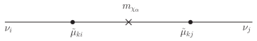
Figure 1: Contribution to the tree level neutrino mass. The cross indicates a mass insertion for the neutralino with a Majorana mass. The blob indicates an RPV mixing.

In our model we have a $9\times 9$ mass matrix for the neutralinos. In the basis $\{\tilde{B},\tilde{W},\tilde{H}_{U_{1}},\tilde{H}_{U_{2}},\nu_{I}\}$, where we neglect the effects of non-renormalizable operators, it is given by

$$M^{N}=\begin{pmatrix}M_{1}&0&m_{Z}s_{W}\hat{v}_{u_{1}}&m_{Z}s_{W}\hat{v}_{u_{2}}&-m_{Z}s_{W}\hat{v}_{I}\\[3.0pt] 0&M_{2}&-m_{Z}c_{W}\hat{v}_{u_{1}}&-m_{Z}c_{W}\hat{v}_{u_{2}}&m_{Z}c_{W}\hat{v}_{I}\\[3.0pt] m_{Z}s_{W}\hat{v}_{u_{1}}&-m_{Z}c_{W}\hat{v}_{u_{1}}&0&0&\mu_{1I}\\[3.0pt] m_{Z}s_{W}\hat{v}_{u_{2}}&-m_{Z}c_{W}\hat{v}_{u_{2}}&0&0&\mu_{2I}\\[3.0pt] -m_{Z}s_{W}\hat{v}_{I}^{T}&m_{Z}c_{W}\hat{v}_{I}^{T}&\mu_{1I}^{T}&\mu_{2I}^{T}&0_{5\times 5}\\ \end{pmatrix},$$ (8)

where $M_{1}$ is the Bino mass, $M_{2}$ is the Wino mass, $\hat{v}_{x}=v_{x}/v$, $c_{W}\equiv\cos\theta_{W}$, $s_{W}\equiv\sin\theta_{W}$ and $\theta_{W}$ is the Weinberg angle. Note that none of the angles between the five-vectors $v_{I}$, $\mu_{1I}$ and $\mu_{2I}$ is small. The R-parity conservation limit corresponds to the case where the three vectors are coplanar. Small R-parity breaking manifests itself by the deviation of $v_{I}$ from the plain determined by $\mu_{1I}$ and $\mu_{2I}$. Such deviation can be parametrized by the angle $\xi$ such that

$$\sin\xi=\frac{(\hat{\mu}_{1}\times\hat{\mu}_{2})\cdot\hat{v}}{\sin\chi},$$ (9)

where $\hat{a}$ is a unit vector in the direction of the vector $a$ and the angle

$$\cos\chi=\frac{\sum\mu_{1I}\mu_{2I}}{\mu_{1}\mu_{2}},$$ (10)

measures the alignment of $\mu_{1I}$ and $\mu_{2I}$. The cross product is defined on the three-dimensional space generated by the three five-vectors.

In order to find the masses, the first thing to note is that the mass matrix has rank seven and thus there are two massless states at tree-level. The product of the seven non-vanishing eigenvalues can be extracted from Eq. (8), and reads:

$$\mathrm{det^{\prime}}M^{N}=2\frac{m_{Z}^{2}\,m_{\tilde{\gamma}}}{v^{2}}\,v_{d}^{2}\,\mu_{1}^{2}\,\mu_{2}^{2}\sin^{2}\chi\sin^{2}\xi,$$ (11)

where we have defined $m_{\tilde{\gamma}}=M_{1}c_{W}^{2}+M_{2}s_{W}^{2}$. Note that when $v_{I}$, $\mu_{1I}$, and $\mu_{2I}$ are in the same plane, $\xi=0$ and thus $\mathrm{det^{\prime}}M^{N}=0$.

In order to get an estimate of the masses we consider the electroweak breaking and SUSY breaking scales to be roughly equal and we denote them by $\tilde{m}$. When we consider all the relevant masses to be of order $\tilde{m}$ the product of the seven non-vanishing masses should satisfy: $\mathrm{det^{\prime}}M^{N}\leq\tilde{m}^{6}m_{3}$. where $m_{3}$ is the mass of the heaviest neutrino. In order for the neutrino masses to be within the experimental bounds we thus require

$$\xi^{2}\lesssim\frac{m_{3}}{\tilde{m}},$$ (12)

where we used $\sin\chi\sim 1$. We see that the expression we get is similar to the one for the case of the MSSM [11]. The small angle in the MSSM is the one between the $\mu$ and $v$ vectors while here it is the angle between the plane generated by the two $\mu$-like vectors and $v$.

In order to obtain the neutrino mass matrix we need to diagonalize the $9\times 9$ matrix $M^{N}$. This computation is simplified by considering the hierarchical structure of the matrix to diagonalize:

$$M^{N}=\begin{pmatrix}M_{6\times 6}&\mu_{6\times 3}\\[4.0pt] \mu^{T}_{3\times 6}&0_{3\times 3}\end{pmatrix}\Longrightarrow UM^{N}U^{+}=\begin{pmatrix}M^{\prime}_{6\times 6}&0_{6\times 3}\\[4.0pt] 0_{3\times 6}&m_{\nu\;3\times 3}\end{pmatrix},$$ (13)

where $M\gg\mu$ and therefore we may integrate out the six neutralinos. From now on we work in the basis spanned by $\hat{L}_{I}$ such that $v_{0}=v_{d_{1}}$, $v_{1}=v_{d_{2}}$ and $v_{m}=0$ for $m=2,3,4$. Note that a basis in which all the $v_{I}$’s except one are zero could also be chosen, however, we prefer to keep our results in a more basis independent fashion. To integrate out the neutralinos we use the see-saw mechanism, where $M$ is a Majorana mass and $\mu$ is a Dirac mass, and obtain the eigenvalues:

$$M^{\prime}_{6\times 6}=M_{6\times 6},\qquad m_{\nu\;3\times 3}=\mu^{T}M^{-1}\mu.$$ (14)

Now, defining the following ratios,

$$\frac{v_{d_{1}}}{v}=\cos\beta\cos\beta_{1},\qquad\frac{v_{d_{2}}}{v}=\cos\beta\sin\beta_{1},\qquad\frac{v_{u_{1}}}{v}=\sin\beta\cos\beta_{2},\qquad\frac{v_{u_{2}}}{v}=\sin\beta\sin\beta_{2},$$ (15)

where $\beta$ is the usual angle defined by the ratio $v_{u}/v_{d}=\tan\beta$. We find the neutrino mass matrix:

$$(m_{\nu})_{ij} = \frac{X}{\Delta\mu^{2}}\left[\mu_{1i}\tilde{\mu}_{2}-\mu_{2i}\tilde{\mu}_{1}\right]\left[\mu_{1j}\tilde{\mu}_{2}-\mu_{2j}\tilde{\mu}_{1}\right]$$ (16)

where

$$X\equiv\frac{m_{\tilde{\gamma}}m_{Z}^{2}\cos^{2}\beta}{M_{1}M_{2}\Delta\mu^{2}+m_{\tilde{\gamma}}m_{Z}^{2}\sin(2\beta)(\tilde{\mu}_{1}\sin\beta_{2}-\tilde{\mu}_{2}\cos\beta_{2})}\sim\frac{\cos^{2}\beta}{\tilde{m}},$$ (17)

and we have defined,

$$\tilde{\mu}_{i}\equiv\mu_{1d_{i}}\sin\beta_{1}-\mu_{2d_{i}}\cos\beta_{1},\qquad\Delta\mu^{2}\equiv\mu_{2d_{2}}\mu_{1d_{1}}-\mu_{1d_{2}}\mu_{2d_{1}}.$$ (18)

In the last step of Eq. (17) we have taken all the relevant masses to be $\tilde{m}$.

The tree level neutrino masses are the eigenvalues of the rank one matrix in Eq. (16) and therefore there is just one massive neutrino:

$$m_{3}=\frac{X}{\Delta\mu^{2}}(\tilde{\mu}_{2}\vec{\mu}_{1}-\tilde{\mu}_{1}\vec{\mu}_{2})^{2}=\frac{X}{\Delta\mu^{2}}\mu_{1}^{2}\mu_{2}^{2}\sin^{2}\chi\sin^{2}\xi,\qquad m_{1}=m_{2}=0,$$ (19)

where $\vec{\mu}_{i}=\mu_{ij}$. We define in the following $m_{3}>m_{2}>m_{1}$. As expected, the tree level neutrino mass is quadratically proportional to the small parameter that measures the RPV.

4 Loop contributions to the neutrino mass matrix

The neutrino mass matrix receives contributions from loop diagrams with $\Delta L=2$. There are one loop contributions due to RPV couplings that are present also in models with one pair of Higgs doublets. They have already been thoroughly studied (see for example [13, 17, 18]), and we collect them in Appendix B for completeness.

Here we concentrate on the new diagrams that arise only once the second pair of Higgs doublets is introduced. Strictly speaking, the only new term that is introduced is $\tilde{\lambda}$. Yet, below we also consider effects that are due to the extended $B$-term, namely $\tilde{B}$, which has been defined in (A). We find that the new effects that are generated by the new $\tilde{\lambda}$ term in the superpotential enter the neutrino masses only at two loops. Roughly speaking, this is because the $\tilde{\lambda}$ term does not involve any neutrinos. Thus it only breaks lepton number by one unit in the charged lepton sector and the transformation of this breaking into the neutrinos appears at one loop. Since we need two of them, we end up with a two loop effect.

The effects of the $\tilde{B}$ coupling on the neutrino mass matrix arise both at one and two loops. The one loop effect is collected in Appendix B. Here we include some of the results for two loop diagrams in order to give an estimate of their possible importance. In general, we expect such two loop effects to be smaller than the one loop effects that the MSSM also presents. Yet, since the coefficients $\tilde{\lambda}_{k}$ are less constrained than the usual RPV coefficients, these two loop diagrams could give important contributions to the neutrino mass matrix.

There are two types of effects that we call separable and non-separable two loop contributions to the neutrino matrix. We study them both below.

4.1 Separable contributions

For the separable contributions we study the Dirac-like neutrino-neutralino mixing (see Fig. 2). We define an effective coupling for this mixing at first order,

$$i\mu^{\text{Dirac}}_{i\alpha}=i\mu^{\tilde{\lambda}}_{i\alpha}+i\mu^{\tilde{B}}_{i\alpha}.$$ (20)

The effective coupling $\mu^{\tilde{\lambda}}_{i\alpha}$ corresponds to the diagram in Fig. 2(a), and can be expressed as:

$$\mu^{\tilde{\lambda}}_{i\alpha}=\frac{1}{8\pi^{2}}\sum_{m}g\tilde{\lambda}_{i}(Z_{-}^{3m}Z_{N}^{4\alpha}-Z_{-}^{2m}Z_{N}^{5\alpha})^{*}Z_{-}^{1m}\frac{m_{\chi_{m}}\Delta^{2}m_{\tilde{l}_{i}}}{m_{\tilde{l}_{i}}^{2}}\approx\frac{3}{8\pi^{2}}g\tilde{\lambda}_{i}m_{l_{i}},$$ (21)

where the $Z$’s refer to the appropriate mixing matrices defined as in the MSSM [14, 15, 16] but enlarged so that they accommodate the extra particle states of our model. In the last step, we have set $\Delta m_{\tilde{l}_{i}}^{2}\approx 2m_{l_{i}}\tilde{m}$ and $m_{\tilde{l}_{i}}\sim m_{\chi_{m}}\sim\tilde{m}$. The effective coupling $\mu^{\tilde{B}}_{i\alpha}$ is represented in Fig. 2(b) and can be expressed as

$$\mu^{\tilde{B}}_{i\alpha}=i\sum_{n,k}g^{2}\tilde{B}_{ik}C_{1}^{\alpha nki}m_{\chi_{n}}I_{3}(m_{\chi_{n}},m_{\tilde{l}_{i}},m_{H_{k}})\approx\sum_{k}\frac{3}{64\pi^{2}}g^{2}\frac{\tilde{B}_{ik}}{\tilde{m}},$$ (22)

where

$$C_{1}^{\alpha nki}\equiv\tilde{Z}_{-}^{1n}(Z_{H}^{2k}+Z_{H}^{3k})\left[(Z_{N}^{4\alpha}+Z_{N}^{5\alpha})Z_{-}^{1i}-\frac{1}{\sqrt{2}}\left(Z_{N}^{1\alpha}+\frac{g^{\prime}}{g}Z_{N}^{0\alpha}\right)(Z_{-}^{2i}+Z_{-}^{3i})\right],$$ (23)

$\tilde{B}_{ik}$ is defined in Eq. (39) and $I_{3}$ is given in Eq. (58) (Eq. (59) for the equal masses case). In the final step we have taken all the masses to be at the supersymmetry breaking scale and we use $C_{1}^{\alpha nki}\sim 0.5$.

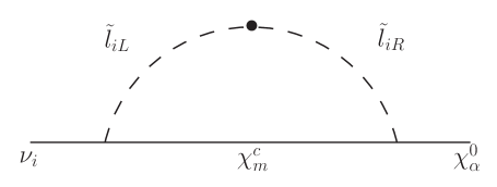
(a) Effective coupling $\mu^{\tilde{\lambda}}_{i\alpha}$.

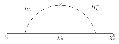
(b) Effective coupling $\mu^{\tilde{B}}_{i\alpha}$.

Figure 2: The blob indicates the mixing between left and right-handed sleptons. The cross indicates the RPV B-vertex.

The separable contribution to the neutrino mass matrix that is proportional to the coupling $\tilde{\lambda}\tilde{\lambda}$ is

$$\left[m_{\nu}\right]_{ij}^{\text{S},\tilde{\lambda}\tilde{\lambda}}=\sum_{\alpha}\frac{\mu^{\tilde{\lambda}}_{i\alpha}\mu^{\tilde{\lambda}}_{j\alpha}}{m_{\chi_{\alpha}^{0}}}\approx\frac{27}{32\pi^{4}}g^{2}\tilde{\lambda}_{i}\tilde{\lambda}_{j}\frac{m_{l_{i}}m_{l_{j}}}{\tilde{m}},$$ (24)

where we used the approximation $m_{\chi_{\alpha}}\sim\tilde{m}$. This contribution is suppressed by two loop factors, two RPV couplings and two leptonic Yukawa couplings. The latter makes this contribution irrelevant in most cases.

Moving to the one that depends on $\tilde{\lambda}_{k}\tilde{B}$ we get

$$\left[m_{\nu}\right]_{ij}^{\text{S},\tilde{\lambda}\tilde{B}}=\sum_{\alpha}\frac{\mu^{\tilde{\lambda}}_{i\alpha}\mu^{\tilde{B}}_{j\alpha}+\mu^{\tilde{B}}_{i\alpha}\mu^{\tilde{\lambda}}_{j\alpha}}{m_{\chi_{\alpha}^{0}}}\approx\sum_{k}\frac{27}{128\pi^{4}}g^{3}\frac{\tilde{\lambda}_{i}\tilde{B}_{jk}m_{l_{i}}+\tilde{\lambda}_{j}\tilde{B}_{ik}m_{l_{j}}}{\tilde{m}^{2}},$$ (25)

where in the last step we consider $m_{\chi_{\alpha}}\sim\tilde{m}$. The suppression factors in this case are given by two loop factors, one Yukawa coupling and the two RPV couplings $\tilde{\lambda}$ and $\tilde{B}$.

Last we show the result for the loop that depends on $\tilde{B}\tilde{B}$. It is given by

$$\left[m_{\nu}\right]_{ij}^{\text{S},\tilde{B}\tilde{B}}=\sum_{\alpha}\frac{\mu^{\tilde{B}}_{i\alpha}\mu^{\tilde{B}}_{j\alpha}}{m_{\chi_{\alpha}^{0}}}\approx\sum_{k,k^{\prime}}\frac{27}{512\pi^{4}}g^{4}\frac{\tilde{B}_{ik}\tilde{B}_{jk^{\prime}}}{\tilde{m}^{3}},$$ (26)

where in the last step $m_{\chi_{\alpha}}\approx\tilde{m}$ is considered. The suppression factors in this case are given by two loop factors and the two RPV couplings $\tilde{\lambda}$, $\tilde{B}$. Since there is no leptonic Yukawa coupling in this case, this is the least suppressed of these contributions.

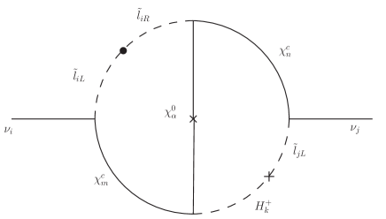
(a) $\tilde{B}\tilde{\lambda}$ diagram

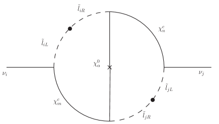
(b) $\tilde{\lambda}\tilde{\lambda}$ diagram

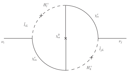
(c) $\tilde{B}\tilde{B}$ diagram

Figure 3: Non-separable two loop diagrams that contribute to neutrino masses. The cross in the bosonic line indicates the RPV $B$ vertex.

4.2 Non-separable contributions

We now move to discuss non-separable two loop diagrams. We have found that there are several of them. We include here three representative cases in order to have an insight of their possible importance. These diagrams are represented in Fig. 3, and we discuss them in turn below.

For the $\tilde{B}\tilde{\lambda}$-diagram in Fig. 3(a) we find

$$\left[m_{\nu}\right]_{ij}^{\text{NS},\tilde{\lambda}\tilde{B}}=\sum_{\alpha,n,m,k}2g^{3}\tilde{\lambda}_{i}^{*}\tilde{B}_{jk}m_{\chi_{\alpha}}m_{\chi_{m}}m_{\chi_{n}}\Delta m_{\tilde{l}_{i}}^{2}C_{2}^{\alpha mnki}I_{6}(m_{\tilde{l}_{i}},m_{\chi_{m}},m_{\chi_{n}},m_{\tilde{l}_{j}},m_{H_{k}},m_{\chi_{\alpha}}),$$ (27)

where

$$\!\!\!\!C_{2}^{\alpha mnki}\equiv$$ (28)

$$\!\!\!\!Z_{-}^{1m}Z_{-}^{1n}(Z_{H}^{2k}+Z_{H}^{3k})^{*}(Z_{-}^{3n}Z_{N}^{4\alpha}-Z_{-}^{2n}Z_{N}^{5\alpha})^{*}\left[(Z_{N}^{4\alpha}+Z_{N}^{5\alpha})Z_{-}^{1i}-\frac{1}{\sqrt{2}}\left(Z_{N}^{1\alpha}+\frac{g^{\prime}}{g}Z_{N}^{0\alpha}\right)(Z_{-}^{2i}+Z_{-}^{3i})\right]$$

and $I_{6}$ is defined in Eq. (67). Note that $C_{2}^{\alpha mnki}$ has several subtractions of $Z$’s and so it could undergo large cancellations. Taking all the masses to be at the electroweak scale, and using $C_{2}^{\alpha mnki}\sim 0.5$, we find

$$\left[m_{\nu}\right]_{ij}^{\text{NS},\tilde{\lambda}\tilde{B}}\approx-\sum_{k}\frac{15.12}{256\pi^{4}}g^{3}\tilde{\lambda}_{i}^{*}\tilde{B}_{jk}\frac{m_{l_{i}}}{\tilde{m}^{2}},$$ (29)

where $I_{6}$ for the equal masses case has been computed in Eq. (68). This contribution to the neutrino mass matrix is suppressed by a lepton mass, the trilinear RPV $\tilde{\lambda}$-coupling, the bilinear supersymmetry-breaking RPV $\tilde{B}$-coupling, and two loop factors.

Moving to the $\tilde{\lambda}\tilde{\lambda}$-diagram in Fig. 3(b) we obtain

$$\left[m_{\nu}\right]_{ij}^{\text{NS},\tilde{\lambda}\tilde{\lambda}}=-\sum_{\alpha,n,m,k}4g^{2}\tilde{\lambda}_{i}^{*}\tilde{\lambda}_{j}^{*}m_{\chi_{\alpha}}m_{\chi_{m}}m_{\chi_{n}}\Delta m_{\tilde{l}_{i}}^{2}\Delta m_{\tilde{l}_{j}}^{2}C_{3}^{\alpha mn}I_{5}(m_{\tilde{l}_{i}},m_{\chi_{m}},m_{\tilde{l}_{j}},m_{\chi_{n}},m_{\chi_{\alpha}}),$$ (30)

where,

$$C_{3}^{\alpha mn}\equiv Z_{-}^{1m}Z_{-}^{1n}(Z_{-}^{3n}Z_{N}^{4\alpha}-Z_{-}^{2n}Z_{N}^{5\alpha})^{*}(Z_{-}^{3m}Z_{N}^{4\alpha}-Z_{-}^{2m}Z_{N}^{5\alpha})^{*}$$ (31)

and $I_{5}$ is defined in Eq. (62). Taking all the masses to be at the electroweak scale, and considering $C_{3}^{\alpha mn}\sim 0.5$, we find:

$$\left[m_{\nu}\right]_{ij}^{\text{NS},\tilde{\lambda}\tilde{\lambda}}\approx\frac{60.48}{256\pi^{4}}g^{2}\tilde{\lambda}_{i}^{*}\tilde{\lambda}_{j}^{*}\frac{m_{l_{i}}m_{l_{j}}}{\tilde{m}},$$ (32)

where $I_{5}$ for the equal mass case has been computed in Eq. (66). This contribution to the neutrino mass matrix is suppressed by two lepton masses, two trilinear RPV $\tilde{\lambda}$-couplings, and two loop factors.

Finally, for the $\tilde{B}\tilde{B}$-diagram in Fig. 3(c), the result reads

$$\left[m_{\nu}\right]_{ij}^{\text{NS},\tilde{B}\tilde{B}}=-\sum_{\alpha,n,m,k,l}g^{2}\tilde{B}_{il}\tilde{B}_{jk}m_{\chi_{\alpha}}m_{\chi_{m}}m_{\chi_{n}}C_{4}^{\alpha mnki}I_{7}(m_{\chi_{m}},m_{H_{l}},m_{\tilde{l}_{i}},m_{\chi_{n}},m_{H_{k}},m_{\tilde{l}_{j}},m_{\chi_{\alpha}}),$$ (33)

where,

$$C_{4}^{\alpha mnkij} \equiv Z_{-}^{1m}Z_{-}^{1n}(Z_{H}^{2k}+Z_{H}^{3k})^{*}(Z_{-}^{3n}Z_{N}^{4\alpha}-Z_{-}^{2n}Z_{N}^{5\alpha})^{*}$$

$$\left[(Z_{N}^{4\alpha}+Z_{N}^{5\alpha})Z_{-}^{1i}-\frac{1}{\sqrt{2}}\left(Z_{N}^{1\alpha}+\frac{g^{\prime}}{g}Z_{N}^{0\alpha}\right)(Z_{-}^{2i}+Z_{-}^{3i})\right]$$

$$(Z_{H}^{2l}+Z_{H}^{3l})^{*}(Z_{-}^{3m}Z_{N}^{4\alpha}-Z_{-}^{2m}Z_{N}^{5\alpha})^{*}\left[(Z_{N}^{4\alpha}+Z_{N}^{5\alpha})Z_{-}^{1j}-\frac{1}{\sqrt{2}}\left(Z_{N}^{1\alpha}+\frac{g^{\prime}}{g}Z_{N}^{0\alpha}\right)(Z_{-}^{2j}+Z_{-}^{3j})\right]$$

and $I_{7}$ is defined in Eq. (69). Note that $C_{4}^{\alpha mnkij}$, just as $C_{2}^{\alpha mnki}$, has several subtractions of $Z$’s and so it could also undergo large cancellations. Taking all the masses to be at the electroweak scale, and using $C_{4}^{\alpha mnkij}\sim 0.5$, we find:

$$\left[m_{\nu}\right]_{ij}^{\text{NS},\tilde{B}\tilde{B}}\approx\sum_{k,l}\frac{3.80}{256\pi^{4}}g^{2}\frac{\tilde{B}_{il}\tilde{B}_{jk}}{\tilde{m}^{3}},$$ (35)

where $I_{7}$ for the equal masses case has been computed in Eq. (70). This contribution to the neutrino mass matrix is suppressed by two bilinear supersymmetry-breaking RPV $\tilde{B}$-couplings, and two loop factors. Note that there is no Yukawa suppression for this diagram.

5 Conclusions

We study new sources of neutrino masses in RPV supersymmetric models with an extra pair of Higgs doublets. In these models there is a new type of RPV term in the superpotential of the form $\tilde{\lambda}_{k}\hat{H}_{D_{1}}\hat{H}_{D_{2}}E_{k}$. Such a term is forbidden in the MSSM since $\lambda$ is antisymmetric in its first two indices. There are also similar new soft SUSY breaking terms. These new terms violate lepton number by one unit and therefore two such terms can induce Majorana neutrino masses.

We find that the tree level effects that arise due to neutrino-neutralino mixing, contribute to the mass of only one neutrino, just like it happens in the MSSM. The value of this mass is quadratically proportional to the small R-parity breaking parameter, which in this case is measured by the deviation of the vector $v$ from planarity with respect to the two $\mu$-like vectors.

At the loop level we find that the new term can contribute to the mass matrix only through two loop diagrams. Thus, in general we expect such terms not to be significant. The estimates of the different diagrams are given in Eqs. (24), (25), (26), (29), (32), and (35). Since they depend on different RPV parameters it is not always clear which one gives the most important contribution. There is, however, one factor that tells them apart which is the amount of Yukawa suppressions. We see that the number of Yukawa factors is the same as the number of $\tilde{\lambda}$ couplings.

If we make the assumption that all RPV parameters are of the same order, that is, $\tilde{B}/\tilde{m}^{2}\sim\tilde{\mu}/\tilde{m}\sim\tilde{\lambda}$, the Yukawa suppression governs the hierarchy. In that case the diagrams without any $\tilde{\lambda}$ couplings are the most important, that is, Eqs. (26) and (35) are expected to give the dominant effect. Nevertheless, the are one loop effects proportional to two $\tilde{B}$’s as in Eq. (55) and thus it is unlikely that the two loop effects will be important.

On the other hand, if we consider another plausible assumption, namely that the only coupling that is significant is $\tilde{\lambda}$, we find that its effect is always suppressed by one small Yukawa, and so it can be important only when $\tilde{\lambda}$ is very large. In this case, we could consider $\tilde{B}/\tilde{m}\sim\tilde{\mu}\sim\tilde{\lambda}m_{l}$ and so the leading contributions will be Eqs. (24), (25), (29), and (32).

Our results can be extended to other similar models. They include models where the extra Higgs states are not just simple duplication of the MSSM one. They may be relevant also to a case study in [20] where non-holomorphic terms like $EH_{D}H_{U}^{\dagger}$ can appear.

To conclude, neutrino masses can be used to put bounds on any model with lepton number violation. In the model we considered, due to the fact that the new term we study couples only to right handed charged leptons, its contribution to neutrino masses is somewhat suppressed. Thus, neutrino masses may not give severe bounds on such models.

Appendix A Feynman Rules

In this Appendix we give the set of Feynman rules in our model necessary for describing all the diagrams studied in this work. As a reference for notation we have followed the MSSM Feynman rules in [14]. For every rule described here, there is one with all arrows reversed and complex conjugated couplings (except for the explicit $i$). In all the cases, fermions are taken to be in their eigenstate basis and sfermions in a basis where they are their supersymmetric partners.

In this model there are RPV bilinear $\mu$-like terms involving a neutrino which arise from Eq. (2), RPV bilinear terms involving neutral scalars and RPV bilinear terms involving charged scalars, both arising from Eq. (4). These vertices and their Feynman rules are represented below

$$i\tilde{\mu}_{ij}^{+}\equiv i(\mu_{1i}Z_{+}^{2j}+\mu_{2i}Z_{+}^{3j})$$ (36)

$$i\tilde{\mu}_{i\alpha}\equiv i(\mu_{1i}Z_{N}^{2\alpha}+\mu_{2i}Z_{N}^{3\alpha})$$ (37)

$$\frac{i}{\sqrt{2}}\tilde{B}_{i\{h,H_{j},A_{j}\}}\equiv\frac{i}{\sqrt{2}}\left[B_{1i}\{Z_{R}^{00},Z_{R}^{0j},iZ_{H}^{0j}\}\right.$$

$$+B_{2i}\{Z_{R}^{10},Z_{R}^{1j},iZ_{H}^{1j}\}+(M_{\tilde{L}}^{2})_{0(1+i)}\{Z_{R}^{20},Z_{R}^{2j},iZ_{H}^{2j}\}$$

$$+\left.(M_{\tilde{L}}^{2})_{1(1+i)}\{Z_{R}^{30},Z_{R}^{3j},iZ_{H}^{3j}\}\right]$$ (38)

$$i\tilde{B}_{ij}\equiv i\left(B_{1i}Z_{H}^{0j}+B_{2i}Z_{H}^{1j}+(M_{\tilde{L}}^{2})_{0(1+i)}Z_{H}^{2j}\right.$$

$$+\left.(M_{\tilde{L}}^{2})_{1(1+i)}Z_{H}^{3j}\right)$$ (39)

where we used

$$(M_{\tilde{L}})_{im}=\lambda_{0(1+i)m}\frac{v_{d_{1}}}{\sqrt{2}}+\lambda_{1(1+i)m}\frac{v_{d_{2}}}{\sqrt{2}}.$$ (40)

The trilinear RPV vertices which include two Higgs fields arise from Eq. (3) and are represented below

$$i\tilde{\lambda}_{k}(Z_{-}^{3j}Z_{N}^{4\alpha}-Z_{-}^{2j}Z_{N}^{5\alpha})$$ (41)

$$\frac{i}{\sqrt{2}}\tilde{\lambda}_{k}(Z_{-}^{3j}\{Z_{R}^{20},Z_{R}^{2i},iZ_{H}^{2i}\}-Z_{-}^{2j}\{Z_{R}^{30},Z_{R}^{3i},iZ_{H}^{3i}\})$$

(42)

$$i\tilde{\lambda}_{k}(Z_{H}^{3i}Z_{N}^{4\alpha}-Z_{H}^{2i}Z_{N}^{5\alpha})$$ (43)

where $\tilde{\lambda}_{k}=\lambda_{01k}=-\lambda_{10k}$.

The triliniear R-parity conserving vertices involving a neutrino are

$$i(\lambda_{0(1+i)i}Z_{H}^{1k}+\lambda_{1(1+i)i}Z_{H}^{2k})$$ (44)

$$i(\lambda_{0(1+i)i}Z_{H}^{1k}+\lambda_{1(1+i)i}Z_{H}^{2k})$$ (45)

$$-i\frac{g}{2}\left(Z_{N}^{1\alpha}-\frac{g^{\prime}}{g}Z_{N}^{0\alpha}\right)$$ (46)

$$i(\lambda_{0(1+i)i}Z_{-}^{2j}+\lambda_{1(1+i)i}Z_{-}^{3j})$$ (47)

$$-igZ_{-}^{1j}$$ (48)

There are other R-parity conserving vertices which we have also extended to include them in our diagrams. They are :

$$-i\frac{g}{2\sqrt{2}}\left[\left(\{Z_{R}^{20},Z_{R}^{2k},iZ_{H}^{2k}\}Z_{N}^{4\alpha}+\{Z_{R}^{30},Z_{R}^{3k},iZ_{H}^{3k}\}Z_{N}^{5\alpha}\right.\right.$$

$$\left.\left.-\{Z_{R}^{00},Z_{R}^{0k},iZ_{H}^{0k}\}Z_{N}^{2\alpha}-\{Z_{R}^{10},Z_{R}^{1k},iZ_{H}^{1k}\}Z_{N}^{3\alpha}\right)\right.$$

$$\left.\left(Z_{N}^{1\beta}-Z_{N}^{0\beta}\frac{g^{\prime}}{g}\right)+\left(\{Z_{R}^{20},Z_{R}^{2k},iZ_{H}^{2k}\}Z_{N}^{4\beta}\right.\right.$$

$$\left.\left.+\{Z_{R}^{30},Z_{R}^{3k},iZ_{H}^{3k}\}Z_{N}^{5\beta}-\{Z_{R}^{00},Z_{R}^{0k},iZ_{H}^{0k}\}Z_{N}^{2\beta}\right.\right.$$

$$\left.\left.-\{Z_{R}^{10},Z_{R}^{1k},iZ_{H}^{1k}\}Z_{N}^{3\beta}\right)\left(Z_{N}^{1\alpha}-Z_{N}^{0\alpha}\frac{g^{\prime}}{g}\right)\right]$$

(49)

$$-ig(Z_{H}^{2k}+Z_{H}^{3k})\left[(Z_{N}^{4\alpha}+Z_{N}^{5\alpha})Z_{-}^{1i}\right.$$

$$\left.-\frac{1}{\sqrt{2}}\left(Z_{N}^{1\alpha}+\frac{g^{\prime}}{g}Z_{N}^{0\alpha}\right)(Z_{-}^{2i}+Z_{-}^{3i})\right]$$ (50)

$$-igZ_{+}^{1i}$$ (51)

$$-i\frac{g}{\sqrt{2}}\left(Z_{N}^{1\alpha}-\frac{g^{\prime}}{g}Z_{N}^{0\alpha}\right)$$ (52)

Appendix B One loop contributions to neutrino masses

Here we collect the results for the one-loop diagrams that contribute to the neutrino masses but do not include the new term in Eq. (3) that we have studied in this work. Due to the extra Higgs fields, the results are not exactly what we have in the MSSM, and thus we show them here.

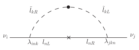
(a) $\lambda\lambda$ loop

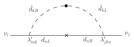
(b) $\lambda^{\prime}\lambda^{\prime}$ loop

Figure 4: $\lambda\lambda$ and $\lambda^{\prime}\lambda^{\prime}$ loops.

The contributions coming from trilinear RPV couplings, which have been already studied in the literature are represented in Fig. 4. Approximate expressions for them, which are enough for our study are:

$$\delta{m_{\nu}}_{ij}^{\lambda\lambda}\approx\frac{1}{8\pi^{2}}\sum_{n,k}\lambda_{ink}\lambda_{jkn}\frac{m_{l_{n}}\Delta m^{2}_{\tilde{l}_{k}}}{m^{2}_{\tilde{l}_{k}}}$$ (53)

$$\delta{m_{\nu}}_{ij}^{\lambda^{\prime}\lambda^{\prime}}\simeq\frac{3}{8\pi^{2}}\sum_{n,k}\lambda^{\prime}_{ink}\lambda^{\prime}_{jkn}\frac{m_{d_{n}}\Delta m^{2}_{\tilde{d}_{k}}}{m^{2}_{\tilde{d}_{k}}}$$ (54)

The soft supersymmetric breaking RPV terms combined in $\tilde{B}_{ik}$ and $\tilde{B}_{i\{h,H_{j},A_{j}\}}$, defined in Eqs. (39) and (A) respectively, also produce contributions to the neutrino masses at the loop level as represented in Fig. 5(a).

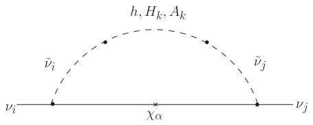
(a) BB contribution to the neutrino mass matrix

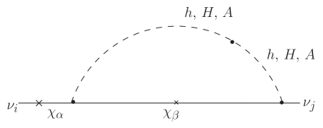
(b) $\mu$B contribution to the neutrino mass matrix

Figure 5: $BB$ and $\mu B$ loops.

The one loop contribution is given by

$$\delta{m_{\nu}}_{ij}^{BB} = \sum_{\alpha}\frac{g^{2}}{4}\left(Z_{N}^{0\alpha}-\frac{g^{\prime}}{g}Z_{N}^{1\alpha}\right)^{2}\left[\tilde{B}_{ih}\tilde{B}_{jh}I_{4}(m_{h},m_{\tilde{\nu}_{i}},m_{\tilde{\nu}_{j}},m_{\chi_{\alpha}})\right.$$ (55)

$$+ \left.\sum_{k}\tilde{B}_{iH_{k}}\tilde{B}_{jH_{k}}I_{4}(m_{H_{k}},m_{\tilde{\nu}_{i}},m_{\tilde{\nu}_{j}},m_{\chi_{\alpha}})+\sum_{k}\tilde{B}_{iA_{k}}\tilde{B}_{jA_{k}}I_{4}(m_{A_{k}},m_{\tilde{\nu}_{i}},m_{\tilde{\nu}_{j}},m_{\chi_{\alpha}})\right]$$

where $I_{4}$ is defined in Eq. (60).

Finally, we study the $\tilde{\mu}\tilde{B}$ Loops represented in Fig. 5(b). These kind of loops contribute like:

$$\delta{m_{\nu}}_{ij}^{\mu B} = \sum_{\alpha,\beta}\frac{g^{2}}{4}\tilde{\mu}_{i\alpha}\left(Z_{N}^{0\alpha}-\frac{g^{\prime}}{g}Z_{N}^{1\alpha}\right)\frac{m_{\chi_{\beta}}}{m_{\chi_{\alpha}}}\left\{\tilde{B}_{jh}\left[\left(Z_{R}^{20}Z_{N}^{4\alpha}+Z_{R}^{30}Z_{N}^{5\alpha}-Z_{R}^{10}Z_{N}^{3\alpha}\right)\frac{}{}\right.\right.$$ (56)

$$\left.\left.\left(Z_{N}^{1\beta}-\frac{g^{\prime}}{g}Z_{N}^{0\beta}\right)+\left(Z_{R}^{20}Z_{N}^{4\beta}+Z_{R}^{30}Z_{N}^{5\beta}-Z_{R}^{00}Z_{N}^{2\beta}-Z_{R}^{10}Z_{N}^{3\beta}\right)\left(Z_{N}^{1\alpha}-\frac{g^{\prime}}{g}Z_{N}^{0\alpha}\right)\right]\right.$$

$$\left.I_{3}(m_{\chi_{\beta}},m_{\tilde{\nu}},m_{h})+\sum_{k}\tilde{B}_{jH_{k}}\left[\left(Z_{R}^{2k}Z_{N}^{4\alpha}+Z_{R}^{3k}Z_{N}^{5\alpha}\right)\left(Z_{N}^{1\beta}-\frac{g^{\prime}}{g}Z_{N}^{0\beta}\right)\right.\right.$$

$$\left.\left.+\left(Z_{R}^{2k}Z_{N}^{4\beta}+Z_{R}^{3k}Z_{N}^{5\beta}-Z_{R}^{0k}Z_{N}^{2\beta}-Z_{R}^{1k}Z_{N}^{3\beta}\right)\left(Z_{N}^{1\alpha}-\frac{g^{\prime}}{g}Z_{N}^{0\alpha}\right)\right]\right.$$

$$\left.I_{3}(m_{\chi_{\beta}},m_{\tilde{\nu}},m_{H_{k}})+\sum_{k}\tilde{B}_{jA_{k}}\left[\left(Z_{H}^{2k}Z_{N}^{4\alpha}+Z_{H}^{3k}Z_{N}^{5\alpha}\right)\left(Z_{N}^{1\beta}-\frac{g^{\prime}}{g}Z_{N}^{0\beta}\right)\right.\right.$$

$$\left.\left.+\left(Z_{H}^{2k}Z_{N}^{4\beta}+Z_{H}^{3k}Z_{N}^{5\beta}-Z_{H}^{0k}Z_{N}^{2\beta}-Z_{H}^{1k}Z_{N}^{3\beta}\right)\left(Z_{N}^{1\alpha}-\frac{g^{\prime}}{g}Z_{N}^{0\alpha}\right)\right]\right.$$

$$\left.I_{3}(m_{\chi_{\beta}},m_{\tilde{\nu}},m_{A_{k}})\frac{}{}\right\}+(i\leftrightarrow j)$$

where $\tilde{\mu}_{i\alpha}$ is defined in Eq. (36). Note that in this result we have neglected terms which are proportional to the tree-level masses.

Appendix C Loop integrals

Here we collect some loop integrals that we have used throughout this work. For all of the integrals a positive and infinitesimal imaginary part is assumed in the propagators.

$$I_{2}(m_{1},m_{2}) \equiv \frac{1}{i}\int\frac{d^{4}p}{(2\pi)^{4}}\frac{1}{p^{2}-m_{1}^{2}}\frac{1}{p^{2}-m_{2}^{2}}=-\frac{1}{16\pi^{2}}\frac{m_{1}^{2}}{m_{1}^{2}-m_{2}^{2}}\ln\frac{m_{1}^{2}}{m_{2}^{2}}$$ (57)

$$I_{3}(m_{1},m_{2},m_{3}) \equiv \frac{1}{i}\int\frac{d^{4}p}{(2\pi)^{4}}\frac{1}{p^{2}-m_{1}^{2}}\frac{1}{p^{2}-m_{2}^{2}}\frac{1}{p^{2}-m_{3}^{2}}=\frac{1}{m_{1}^{2}-m_{2}^{2}}\left[I_{2}(m_{1},m_{3})-I_{2}(m_{2},m_{3})\right].$$ (58)

When all masses are equal we get:

$$I_{3}(m,m,m)=\frac{1}{32\pi^{2}}\frac{1}{m^{2}}.$$ (59)

Next we have

$$I_{4}(m_{1},m_{2},m_{3},m_{4}) \equiv \frac{1}{i}\int\frac{d^{4}p}{(2\pi)^{4}}\frac{1}{p^{2}-m_{1}^{2}}\frac{1}{p^{2}-m_{2}^{2}}\frac{1}{p^{2}-m_{3}^{2}}\frac{1}{p^{2}-m_{4}^{2}}$$

$$= \frac{1}{m_{1}^{2}-m_{2}^{2}}\left[I_{3}(m_{1},m_{3},m_{4})-I_{3}(m_{2},m_{3},m_{4})\right].$$ (60)

For the case where the masses are equal

$$I_{4}(m,m,m,m)=\frac{-1}{96\pi^{2}}\frac{1}{m^{4}}.$$ (61)

Moving on

$$I_{5}(m_{1},m_{2},m_{3},m_{4},m_{5})=$$

$$\frac{1}{m_{2}m_{4}m_{5}}\int\frac{d^{4}q}{(2\pi)^{4}}\frac{d^{4}k}{(2\pi)^{4}}\frac{m_{2}m_{3}m_{5}+m_{2}k^{2}-m_{5}q^{2}+(m_{4}-m_{2}+m_{5})q\cdot k}{(q^{2}-m_{1}^{2})^{2}(q^{2}-m_{2}^{2})((q-k)^{2}-m_{3}^{2})^{2}((q-k)^{2}-m_{4}^{2})(k^{2}-m_{5}^{2})}$$

$$=\frac{\partial}{\partial m_{1}^{2}}\frac{\partial}{\partial m_{3}^{2}}\left\{\frac{1}{m_{1}^{2}-m_{2}^{2}}\frac{1}{m_{3}^{2}-m_{4}^{2}}J_{3}(m_{5},m_{2},m_{4},m_{1},m_{3},m_{5})\right.$$

$$\left.+\frac{1}{m_{1}^{2}-m_{2}^{2}}\frac{1}{m_{4}^{2}-m_{3}^{2}}J_{3}(m_{5},m_{2},m_{4},m_{1},m_{4},m_{5})+\frac{1}{m_{2}^{2}-m_{1}^{2}}\frac{1}{m_{3}^{2}-m_{4}^{2}}J_{3}(m_{5},m_{2},m_{4},m_{2},m_{3},m_{5})\right.$$

$$\left.+\frac{1}{m_{2}^{2}-m_{1}^{2}}\frac{1}{m_{4}^{2}-m_{3}^{2}}J_{3}(m_{5},m_{2},m_{4},m_{2},m_{4},m_{5})\right\}\,,$$ (62)

where we have defined

$$J_{3}(m_{1},m_{2},m_{3},m_{A},m_{B},m_{C}) \equiv$$ (63)

$$\frac{1}{m_{2}m_{4}m_{5}}\int\frac{d^{4}q}{(2\pi)^{4}}\frac{d^{4}k}{(2\pi)^{4}}\frac{m_{1}m_{2}m_{3}+m_{2}k^{2}-m_{1}q^{2}+(m_{3}+m_{1}-m_{2})q\cdot k}{(q^{2}-m_{A}^{2})((k-q)^{2}-m_{B}^{2})(k^{2}-m_{C}^{2})}$$

$$=\frac{(m_{1}+m_{2}+m_{3})}{2m_{1}m_{2}m_{3}}T_{2}(m_{A},m_{B})-\frac{(m_{1}-m_{2}+m_{3})}{2m_{1}m_{2}m_{3}}T_{2}(m_{A},m_{C})-\frac{(m_{1}+m_{2}-m_{3})}{2m_{1}m_{2}m_{3}}T_{2}(m_{B},m_{C})$$

$$+\left(1+\frac{m_{3}\left(m_{A}^{2}-m_{B}^{2}+m_{C}^{2}\right)+m_{1}\left(-m_{A}^{2}-m_{B}^{2}+m_{C}^{2}\right)+m_{2}\left(-m_{A}^{2}+m_{B}^{2}+m_{C}^{2}\right)}{2m_{1}m_{2}m_{3}}\right)$$

$$T_{3}(m_{A},m_{B},m_{C}),$$

and

$$T_{2}(m_{1},m_{2}) \equiv (2\pi)^{-2D}\int\frac{d^{D}k\,d^{D}l}{(k^{2}-m_{1}^{2})(l^{2}-m_{2}^{2})}=-\frac{(\mu^{2})^{4-D}}{(4\pi)^{D}}\left(\Gamma\left(1-D/2\right)\right)^{2}(m_{1}^{2}m_{2}^{2})^{D/2-1}\,$$ (64)

$$T_{3}(m_{1},m_{2},m_{3}) \equiv \frac{(\mu^{2})^{4-D}}{(2\pi)^{2D}}\int\frac{d^{D}k\,d^{D}l}{(k^{2}-m_{1}^{2})((k-l)^{2}-m_{2}^{2})(l^{2}-m_{3}^{2})}\,,$$ (65)

where $\mu$ is the dimensional regularization scale, and $T_{3}$ has been evaluated in [19]. Note that even though both $T_{2}$ and $T_{3}$ diverge and are therefore dimensional regularization scale dependent, the total sum of all their contributions in Eq. (62) is finite and scale independent. The same thing happens for Eqs. (67) and (69). For the case where all the masses are equal we get

$$I_{5}(m,m,m,m,m,) = \frac{1}{(4\pi)^{4}}\frac{1}{m^{6}}\left\{-\frac{5}{12}+3\int_{0}^{1}dx(1-x)x^{3}\int_{0}^{1}dy\frac{(1-y)^{2}y}{2((1-x)x(1-y)+y)^{3}}\right\}$$ (66)

$$\approx -\frac{1}{(4\pi)^{4}}\frac{0.14}{m^{6}},$$

where in the last step the integral is computed numerically. Next we have

$$I_{6}(m_{1},m_{2},m_{3},m_{4},m_{5},m_{6})=\frac{1}{m_{2}m_{3}m_{6}}\int\frac{d^{4}q}{(2\pi)^{4}}\frac{d^{4}k}{(2\pi)^{4}}$$

$$\frac{m_{2}m_{3}m_{6}+m_{2}k^{2}-m_{6}q^{2}+(m_{3}-m_{2}+m_{6})q\cdot k}{(q^{2}-m_{1}^{2})^{2}(q^{2}-m_{2}^{2})((q-k)^{2}-m_{3}^{2})((q-k)^{2}-m_{4}^{2})((q-k)^{2}-m_{5}^{2})(k^{2}-m_{6}^{2})}$$

$$=\frac{\partial}{\partial m_{1}^{2}}\left\{\frac{J_{3}(m_{6},m_{2},m_{3},m_{1},m_{3},m_{6})}{(m_{1}^{2}-m_{2}^{2})(m_{3}^{2}-m_{4}^{2})(m_{3}^{2}-m_{5}^{2})}+\frac{J_{3}(m_{6},m_{2},m_{3},m_{1},m_{4},m_{6})}{(m_{1}^{2}-m_{2}^{2})(m_{4}^{2}-m_{3}^{2})(m_{4}^{2}-m_{5}^{2})}\right.$$

$$\hskip 93.89409pt+\left.\frac{J_{3}(m_{6},m_{2},m_{3},m_{1},m_{5},m_{6})}{(m_{1}^{2}-m_{2}^{2})(m_{5}^{2}-m_{3}^{2})(m_{5}^{2}-m_{4}^{2})}+\frac{J_{3}(m_{6},m_{2},m_{3},m_{2},m_{3},m_{6})}{(m_{2}^{2}-m_{1}^{2})(m_{3}^{2}-m_{4}^{2})(m_{3}^{2}-m_{5}^{2})}\right.$$

$$\hskip 93.89409pt-\left.\frac{J_{3}(m_{6},m_{2},m_{3},m_{2},m_{4},m_{6})}{(m_{2}^{2}-m_{1}^{2})(m_{4}^{2}-m_{3}^{2})(m_{4}^{2}-m_{5}^{2})}+\frac{J_{3}(m_{6},m_{2},m_{3},m_{2},m_{5},m_{6})}{(m_{2}^{2}-m_{1}^{2})(m_{5}^{2}-m_{3}^{2})(m_{5}^{2}-m_{4}^{2})}\right\}\,.$$ (67)

For the case where all the masses are equal we get

$$I_{6}(m,m,m,m,m,m)=I_{5}(m,m,m,m,m).$$ (68)

Last we have,

$$I_{7}(m_{1},m_{2},m_{3},m_{4},m_{5},m_{6},m_{7})=\int\frac{d^{4}q}{(2\pi)^{4}}\frac{d^{4}k}{(2\pi)^{4}}$$

$$\frac{m_{1}m_{4}m_{7}+m_{1}k^{2}-m_{7}q^{2}+(m_{4}-m_{1}+m_{7})q\cdot k}{(q^{2}-m_{1}^{2})(q^{2}-m_{2}^{2})(q^{2}-m_{3}^{2})((q-k)^{2}-m_{4}^{2})((q-k)^{2}-m_{5}^{2})((q-k)^{2}-m_{6}^{2})(k^{2}-m_{7}^{2})}$$

$$=\frac{J_{3}(m_{7},m_{1},m_{4},m_{1},m_{4},m_{7})}{(m_{1}^{2}-m_{2}^{2})(m_{1}^{2}-m_{3}^{2})(m_{4}^{2}-m_{5}^{2})(m_{4}^{2}-m_{6}^{2})}+\frac{J_{3}(m_{7},m_{1},m_{4},m_{1},m_{5},m_{7})}{(m_{1}^{2}-m_{2}^{2})(m_{1}^{2}-m_{3}^{2})(m_{5}^{2}-m_{4}^{2})(m_{5}^{2}-m_{6}^{2})}$$

$$+\frac{J_{3}(m_{7},m_{1},m_{4},m_{1},m_{6},m_{7})}{(m_{1}^{2}-m_{2}^{2})(m_{1}^{2}-m_{3}^{2})(m_{6}^{2}-m_{4}^{2})(m_{6}^{2}-m_{5}^{2})}+\frac{J_{3}(m_{7},m_{1},m_{4},m_{2},m_{4},m_{7})}{(m_{2}^{2}-m_{1}^{2})(m_{2}^{2}-m_{3}^{2})(m_{4}^{2}-m_{5}^{2})(m_{4}^{2}-m_{6}^{2})}$$

$$+\frac{J_{3}(m_{7},m_{1},m_{4},m_{2},m_{5},m_{7})}{(m_{2}^{2}-m_{1}^{2})(m_{2}^{2}-m_{3}^{2})(m_{5}^{2}-m_{4}^{2})(m_{5}^{2}-m_{6}^{2})}+\frac{J_{3}(m_{7},m_{1},m_{4},m_{2},m_{6},m_{7})}{(m_{2}^{2}-m_{1}^{2})(m_{2}^{2}-m_{3}^{2})(m_{6}^{2}-m_{4}^{2})(m_{6}^{2}-m_{5}^{2})}$$

$$+\frac{J_{3}(m_{7},m_{1},m_{4},m_{3},m_{4},m_{7})}{(m_{3}^{2}-m_{1}^{2})(m_{3}^{2}-m_{2}^{2})(m_{4}^{2}-m_{5}^{2})(m_{4}^{2}-m_{6}^{2})}+\frac{J_{3}(m_{7},m_{1},m_{4},m_{3},m_{5},m_{7})}{(m_{3}^{2}-m_{1}^{2})(m_{3}^{2}-m_{2}^{2})(m_{5}^{2}-m_{4}^{2})(m_{5}^{2}-m_{6}^{2})}$$

$$+\frac{J_{3}(m_{7},m_{1},m_{4},m_{3},m_{5},m_{7})}{(m_{3}^{2}-m_{1}^{2})(m_{3}^{2}-m_{2}^{2})(m_{6}^{2}-m_{4}^{2})(m_{6}^{2}-m_{5}^{2})}\,.$$ (69)

For the case where all the masses are equal we get

$$I_{7}(m,m,m,m,m,m,m)=I_{5}(m,m,m,m,m).$$ (70)

References

[1]
For a review on neutrino physics see, for example,
R. N. Mohapatra, S. Antusch, K. S. Babu, G. Barenboim, M. -C. Chen, A. de Gouvea, P. de Holanda and B. Dutta et al.,
Rept. Prog. Phys. 70, 1757 (2007)
[hep-ph/0510213].
[2]
Y. Fukuda et al. [Super-Kamiokande Collaboration],
Phys. Rev. Lett. 81, 1562 (1998)
[hep-ex/9807003].
W. A. Mann [Soudan-2 Collaboration],
Nucl. Phys. Proc. Suppl. 91, 134 (2001)
[hep-ex/0007031].
Q. R. Ahmad et al. [SNO Collaboration],
Phys. Rev. Lett. 89, 011301 (2002)
[nucl-ex/0204008].
B. T. Cleveland, T. Daily, R. Davis, Jr., J. R. Distel, K. Lande, C. K. Lee, P. S. Wildenhain and J. Ullman,
Astrophys. J. 496, 505 (1998).
[3]
M. C. Gonzalez-Garcia and C. Pena-Garay,
Phys. Rev. D 68, 093003 (2003)
[hep-ph/0306001].
M. Maltoni, T. Schwetz, M. A. Tortola and J. W. F. Valle,
Phys. Rev. D 68, 113010 (2003)
[hep-ph/0309130].
A. Bandyopadhyay, S. Choubey, S. Goswami,
Phys. Lett. B 583, 134 (2004)
[hep-ph/0309174].
[4]
J. Beringer et al. [Particle Data Group Collaboration],
Phys. Rev. D 86, 010001 (2012).
[5]
We do not reference here all the literature on neutrinos within RPV SUSY:
C. S. Aulakh and R. N. Mohapatra,
Phys. Lett. B 119, 136 (1982).
L. J. Hall and M. Suzuki,
Nucl. Phys. B 231, 419 (1984).
F. Borzumati, Y. Grossman, E. Nardi and Y. Nir,
Phys. Lett. B 384, 123 (1996)
[hep-ph/9606251].
S. Rakshit, G. Bhattacharyya and A. Raychaudhuri,
Phys. Rev. D 59, 091701 (1999)
[hep-ph/9811500].
S. Davidson and M. Losada,
JHEP 0005, 021 (2000)
[hep-ph/0005080].
S. Davidson and M. Losada,
Phys. Rev. D 65, 075025 (2002)
[hep-ph/0010325].
[6]
T. Lee, Phys. Rev., vol D8, pp. 1226-1239, 1973.
J. F. Gunion, H. E. Haber, G. L. Kane and S. Dawson,
Front. Phys. 80, 1 (2000).
G. Branco, P. Ferreira, L. Lavoura, M. Rebelo, M. Sher, et al., Phys.Rept., vol. 516, pp. 1’Äì102, 2012, 1106.0034
[7]
J. R. Espinosa and M. Quiros,
Phys. Lett. B 302, 51 (1993)
[hep-ph/9212305].
G. D. Kribs, E. Poppitz and N. Weiner,
Phys. Rev. D 78, 055010 (2008)
[arXiv:0712.2039 [hep-ph]].
D. S. M. Alves, P. J. Fox and N. Weiner,
arXiv:1207.5522 [hep-ph].
[8]
D. S. M. Alves, P. J. Fox and N. J. Weiner,
arXiv:1207.5499 [hep-ph].
[9]
Y. Grossman and H. E. Haber,
Phys. Rev. D 59, 093008 (1999)
[hep-ph/9810536].
[10]
L. E. Ibanez and G. G. Ross,
Nucl. Phys. B 368, 3 (1992).
[11]
T. Banks, Y. Grossman, E. Nardi and Y. Nir,
Phys. Rev. D 52, 5319 (1995)
[hep-ph/9505248].
[12]
F. Borzumati, Y. Grossman, E. Nardi and Y. Nir,
Phys. Lett. B 384, 123 (1996)
[hep-ph/9606251].
[13]
Y. Grossman and S. Rakshit,
Phys. Rev. D 69, 093002 (2004)
[hep-ph/0311310].
[14]
H. K. Dreiner, H. E. Haber, S. P. Martin and ,
Phys. Rept. 494, 1 (2010)
[arXiv:0812.1594 [hep-ph]].
[15]
J. Rosiek,
hep-ph/9511250.
[16]
S. P. Martin,
In *Kane, G.L. (ed.): Perspectives on supersymmetry II* 1-153
[hep-ph/9709356].
[17]
S. Davidson and M. Losada,
JHEP 0005, 021 (2000)
[hep-ph/0005080].
[18]
S. Davidson and M. Losada,
Phys. Rev. D 65, 075025 (2002)
[hep-ph/0010325].
[19]
C. Ford, I. Jack and D. R. T. Jones,
Nucl. Phys. B 387, 373 (1992)
[Erratum-ibid. B 504, 551 (1997)]
[hep-ph/0111190].
[20]
C. Csaki, E. Kuflik and T. Volansky,
arXiv:1309.5957 [hep-ph].