Exploring the Phase Structure and Thermodynamics of QCD

Abstract:

We put forward a Polyakov-loop extended quark meson model, where matter as well as glue fluctuations are taken into account, cf. [1]. The latter are included via a Polyakov-loop potential. Usually such a glue potential is based on Yang-Mills lattice data only. We show that a parametrisation of unquenching effects as proposed in [2], together with the inclusion of fluctuations via the functional renormalisation group [3, 4], accounts for the relevant dynamics. This is demonstrated by a comparison of order parameters and thermodynamic observables to recent lattice results at vanishing chemical potential, where we find very good agreement.

bjcolrgb1,0.205,0.80

1 Introduction

The understanding of the phase structure and thermodynamics of Quantum Chromodynamics (QCD) has been a major aim of theoretical as well as experimental high-energy physics over the last years. Running and planned experiments at CERN, RHIC, NICA and FAIR will provide us with important insights into the behaviour of strongly interacting matter under extreme conditions, such as high temperatures and densities. For a comprehensive theoretical understanding of these systems, it is necessary to employ non-perturbative techniques. These allow to study the physics of, e.g., the chiral and deconfinement phase transitions in QCD. Functional methods, such as the Functional Renormalisation Group (FRG) provide one such tool. The recent years have seen a lot of progress in this area: for example it has been demonstrated that the FRG is a suitable tool to study QCD at finite temperature as well as at finite chemical potentials [5, 6, 7, 8].

While first-principles studies of QCD are possible within the FRG framework by now, they still pose a formidable task. Thus, it has proven fruitful to employ functional techniques also to low-energy effective models, which share some aspects with the full theory while being more tractable. Furthermore, it has been demonstrated that these effective models can be related to QCD in a systematic fashion, see e.g. [2, 3, 9] for a detailed discussion. In the present work we use the Polyakov–quark-meson (PQM) model, as one representative of Polyakov-loop enhanced chiral models, see e.g. [10, 11, 12, 13, 14], which is known to describe the chiral properties of QCD very well. Furthermore, the coupling to the Polyakov-loop provides a statistical implementation of confinement. Unquenching effects are included as in [1, 2], see also our discussion in Sec. 3.

A different first-principles approach to QCD are lattice simulations. These have shed light on the phase structure and bulk thermodynamics, especially at vanishing chemical potential, where the infamous sign problem is absent. In this region, results at physical masses [15, 16] and in the continuum limit are available by now [17, 18, 19]. These results can be used to scrutinise results from other approaches, allowing us to determine whether all relevant physical effects have been included, for a more detailed discussion see [1].

2 QCD at Low Energies: The Polyakov-Quark-Meson Truncation

We briefly recapitulate the Polyakov–quark-meson (PQM) model [14] as a low-energy effective theory for QCD. For a more detailed discussion, the reader is referred to e.g. [3, 4, 20, 21]. The Euclidean Lagrangian of this model, including a flavour-blind chemical potential $\mu$, reads

$$\mathcal{L}_{\rm PQM} = \bar{q}\left({D\!\hbox to0.0pt{\hss/}}\,+h\,T^{a}(\sigma_{a}+i\gamma_{5}\pi_{a})+\mu\gamma_{0}\right)q+\ \mathcal{L}_{m}+\ V_{\rm glue}(\Phi,\bar{\Phi};t)\,.$$ (1)

Here, the chiral sector is given by the well-known quark-meson model, see e.g. [22] and references therein. It is supplemented by a mesonic Lagrangian [4, 20]

$$\mathcal{L}_{m} = \operatorname{Tr}(\partial_{\mu}\Sigma\partial_{\mu}\Sigma^{\dagger})+U(\rho_{1},\tilde{\rho}_{2})+c\,\xi-\ \operatorname{Tr}\left[C(\Sigma+\Sigma^{\dagger})\right]\,,$$ (2)

where $\Sigma$ is a complex matrix containing the mesonic fields: $\Sigma=\Sigma_{a}T^{a}=(\sigma_{a}+i\pi_{a})T^{a}\,,$ with $\sigma_{a}$ denoting the scalar and $\pi_{a}$ the pseudo-scalar meson nonets. Furthermore, $T^{a}=\lambda^{a}/2\,$ denote the Hermitian generators of the flavour $U(3)$ symmetry, defined via the Gell-Mann matrices. A flavour-blind Yukawa coupling $h$ couples the quark fields to the mesonic sector. In the following we will consider the $(2+1)$-flavour case, hence assuming isospin symmetry in the light sector.

The meson potential $U$ can be expressed via the chiral invariants $\rho_{i}~{}=~{}\operatorname{Tr}\left[(\Sigma\Sigma^{\dagger})^{i}\right]$, $i=1,\,\dots,\,N_{f}$ [23]. In the ($2+1$)-flavour approximation considered here, we restrict ourselves to the two perturbatively renormalisable invariants $\rho_{1}$ and $\tilde{\rho}_{2}=\rho_{2}-\frac{1}{3}\rho_{1}^{2}$. The chiral $U_{A}(1)$ anomaly is included with the help of the ’t Hooft determinant $\xi=\det(\Sigma)+\det(\Sigma^{\dagger})$ [24, 25]. The strength of its coupling, $c$, determines the mass splitting between the $\eta$, $\eta^{\prime}$ and pions, see e.g. [4, 20, 26] for a detailed discussion.

The gauge fields, represented in terms of Polyakov-loop variables, are coupled to the matter sector via the covariant derivative ${D\!\hbox to0.0pt{\hss/}}\,(\Phi)=\gamma_{\mu}\partial_{\mu}-i\,g\gamma_{0}A_{0}(\Phi)$. Integrating out the gluonic degrees of freedom furthermore results in a potential for the Polyakov loops, $V_{\rm glue}(\Phi(A_{0}),\,\bar{\Phi}(A_{0}))$, which is discussed in more detail in the following.

3 Unquenching

Consider the effective action of full QCD, which can be written as

$$\Gamma_{k}=\beta\mathcal{V}V[A_{0}]+\Delta\Gamma_{k}[\bar{A}_{0},\phi]\,,$$ (3)

where $\mathcal{V}$ is the spatial volume and $\beta=1/T$ the inverse temperature. In Eq. (3), the first term denotes the QCD glue potential, encoding the ghost-gluon dynamics in the presence of matter fields. The second term contains the matter contribution coupled to a background gluon field $\bar{A}_{0}$. For brevity, the remaining field content is collected in $\phi$. This part is well-described in terms of low-energy chiral models, such as the PQM model discussed above.

It is important to notice that the QCD glue potential is different from its pure Yang-Mills counterpart: unquenching effects of the matter fields modify the QCD glue potential. In particular, they lower the deconfinement temperature, see also the discussion in [1, 2, 9, 14, 21]. Within effective model studies, different ansätze for this potential are used, which usually are fitted to Yang-Mills lattice data. Obviously, this procedure does not account for the unquenching effects.

By now, first principles FRG calculations of the glue potential in pure Yang-Mills theory as well as 2-flavour QCD in the chiral limit are available [5, 6, 7, 27]. These have revealed striking similarities between the two potentials: apart from a linear rescaling and shift in the critical temperature, their overall shape is very similar. This insight has been used in [2] to derive a simple relation between the reduced temperatures, $t_{\rm YM,glue}=({T-T_{\rm YM,glue}^{\rm cr}})/{T_{\rm YM,glue}^{\rm cr}}$, of the two theories

$$t_{\rm YM}(t_{\rm glue})\approx 0.57\,t_{\rm glue}\,.$$ (4)

In practice, Eq. (4) allows to keep the well-known parametrisations of the Polyakov-loop potential, as proposed e.g. in [12, 28, 29, 30, 31], and include unquenching effects by a simple rescaling of the reduced temperature. In [2] this approach has been used within a mean-field analysis of the PQM model. Already there it was found that the inclusion of the unquenching effects in this simple manner yields results that are very close to the lattice ones. Here, we report on the next step that consists of including quantum and thermal fluctuations via the FRG. A more detailed discussion is provided in [1]. Specifically, we show results for a polynomial version of the Polyakov-loop potential, introduced in [12, 28]

$$\frac{\mathcal{U}_{\rm poly}(\Phi,\bar{\Phi};t)}{T^{4}} = -\frac{b_{2}(t)}{2}\Phi\bar{\Phi}-\ \frac{b_{3}}{6}\left(\Phi^{3}+\bar{\Phi}^{3}\right)+\ \frac{b_{4}}{4}\left(\Phi\bar{\Phi}\right)^{2}\,,$$ (5)

with the (Yang-Mills based) parameters as given in [12]. The remaining open parameter in Eq. (4), $T_{\rm cr}^{\rm glue}$, is fixed by a comparison to the lattice result for the pressure, resulting in $T_{\rm cr}^{\rm glue}=210$ MeV for our FRG computation. A discussion of the parameter dependence of our results can be found in [1].

4 Including Fluctuations

As mentioned above, we include thermal as well as quantum fluctuations with the FRG. It has been shown previously, see e.g. [22], that this is crucial to achieve a realistic description of the phase transition, which is too steep in, e.g., the standard mean-field approximation.

In [1] we have put forward the flow equation for the $(2+1)$-flavour PQM model in the lowest order of a derivative expansion

$$\partial_{t}\Omega_{k} = \frac{k^{5}}{12\pi^{2}}\left\{\sum_{i=1}^{2N_{f}^{2}}\frac{1}{E_{i}}\coth\left(\frac{E_{i}}{2T}\right)-\frac{8N_{c}}{E_{l}}\left[1-N_{l}(T,\mu;\Phi,\bar{\Phi})-N_{\bar{l}}(T,\mu;\Phi,\bar{\Phi})\right]\right.$$ (6)

$$\quad\left.-\frac{4N_{c}}{E_{s}}\left[1-N_{s}(T,\mu;\Phi,\bar{\Phi})-N_{\bar{s}}(T,\mu;\Phi,\bar{\Phi})\right]\right\}\,.$$

Here, the Polyakov-loop enhanced quark/anti-quark occupation numbers are given by

$$N_{q}(T,\mu;\Phi,\bar{\Phi}) = \dfrac{1+2\bar{\Phi}e^{(E_{q}-\mu)/T}+\Phi e^{2(E_{q}-\mu)/T}}{1+3\bar{\Phi}e^{(E_{q}-\mu)/T}+3\Phi e^{2(E_{q}-\mu)/T}+e^{3(E_{q}-\mu)/T}}\,,$$ (7)

and $N_{\bar{q}}(T,\mu;\Phi,\bar{\Phi})\equiv N_{q}(T,-\mu;\bar{\Phi},\Phi)$ for $q=l,s$. Furthermore, the quasi-particle energies of the quarks and mesons are given by $E_{j}=\sqrt{k^{2}+m_{j}^{2}}$, $j~{}\in~{}\{l,\,s,\,i\}$ with $i\in\{\sigma,\,\vec{a_{0}},\,\vec{\kappa},\,f_{0},\,\vec{\pi},\,\vec{K},\,\eta,\,\eta^{\prime}\}$.

For convenience, we use a non-strange–strange basis, where the light and strange quark masses can be expressed in terms of the non-strange, $\sigma_{x}$, and strange, $\sigma_{y}$, condensates and the Yukawa coupling as $m_{l}=h\frac{\sigma_{x}}{2}\,,m_{s}=h\frac{\sigma_{y}}{\sqrt{2}}$ . The meson masses, on the other hand, are defined via eigenvalues of the Hessian of the potential

$$\{m_{j}^{2}\}=\text{eig}\left\{H_{\Sigma}\left(U(\rho_{1},\tilde{\rho}_{2})+c\xi\right)\right\}\,.$$ (8)

Equation (6) encodes the scale dependence of the mesonic couplings via the scale-dependent effective potential $\Omega_{k}$ , while the running of other interactions containing quarks is neglected. The flow equation can be solved once the initial potential is fixed at an ultraviolet scale $\Lambda=1$ GeV, where we expect our truncation to be a reasonable description of QCD, cf. our discussion above. For the details of our numerical method and the used parameters we refer the reader to [1, 4, 32].

Evolving the flow equation from $\Lambda$ to the infrared, $k\to 0$, fluctuations with momenta smaller than $\Lambda$ are included. However, this also implies that high modes with momenta $k>\Lambda$ are neglected. In particular, this translates into a restriction of the tractable temperature range, $\Lambda\gtrsim 2\pi T\,.$ Above this temperature, thermal fluctuations become important also at scales above the cutoff. Therefore, the initial potential $\Omega_{\Lambda}$ is not fully independent of temperature, which becomes quantitatively important in the region $2\pi T\gtrsim\Lambda$. In [1] we have argued that the fermionic contributions are dominant over the bosonic ones in this region. Moreover, we have shown there, how these fermionic temperature fluctuations can be included in the initial action $\Omega_{\Lambda}$ at the cutoff. Our argument relies on the fact that the temperature dependence of the initial potential $\Omega_{\Lambda}$ is also governed by the flow Eq. (6). The finite temperature correction can then be obtained by integrating the vacuum flow from $\Lambda$ to $\bar{\Lambda}\gg 2\pi T$ and subsequently integrating the finite temperature flow down to $k=\Lambda$. The resulting flow is especially easy for the fermionic system, where one can actually use $\bar{\Lambda}=\infty$ . This procedure allows to study thermodynamic observables also at temperatures above the phase transition. We refer the interested reader to [1] for a detailed discussion.

5 Results

Although finite densities are straight-forward to implement in our setup, see also [33] for a discussion of possible issues, we focus in the following on the case of vanishing chemical potential. On the one hand, this is the region where we can benchmark our results with the lattice ones. On the other hand, it also has numerical advantages, since the Polyakov loop and its conjugate coincide in this case $\bar{\Phi}(T,\mu=0)=\Phi(T,\mu=0)$ . This reduces the numerical effort for solving the equations of motions drastically.

The effective potential in the infrared, $\Omega_{k\to 0}$, evaluated at the solution, $\chi_{0}=\left(\sigma_{x},\sigma_{y},\Phi\right)$, of the corresponding equations of motion

$$\left.\frac{d\Omega_{k\to 0}}{d\sigma_{x}}\right|_{\chi_{0}}=\left.\frac{d\Omega_{k\to 0}}{d\sigma_{y}}\right|_{\chi_{0}}=\left.\frac{d\Omega_{k\to 0}}{d\Phi}\right|_{\chi_{0}}=0\,,$$ (9)

will serve as the basis to calculate thermodynamic observables. It is related to the pressure $P(T,\mu)=-(\Omega(T,\mu)-\Omega(0,0))$ with $\Omega(T,\mu)=\Omega_{k\to 0}(T,\mu)|_{\chi_{0}}$, and as such acts as a thermodynamic potential, from which observables can be calculated in the standard manner.

To highlight the importance of fluctuations, we also show results from a standard mean-field calculation, which neglects fluctuations of the mesonic fields. It has been shown that the standard mean-field approximation (MF) misses a contribution stemming from the fermionic vacuum loop. While this term is naturally included in the FRG approach, it can be added to the standard MF, resulting in the so-called extended MF (eMF) [34, 35].

Furthermore, it is our goal to check the proper inclusion of fluctuations as well as unquenching effects. To do so, we compare our results to recent lattice data by the HotQCD [15, 16] and Wuppertal-Budapest collaborations [17, 18, 19].

In the following, we show all our results in terms of the reduced temperature $t=(T-T_{\chi})/T_{\chi}$, where $T_{\chi}$ denotes the chiral transition temperature. This choice allows us to compare the overall shape - and thereby the proper inclusion of the relevant dynamics - of the observables, while a possible mismatch of the critical temperature is scaled out. Note, however, that the scale mismatch is $\leq 10\%$ within our FRG calculation, see Tab. 1.

5.1 Phase Structure

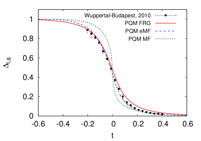
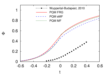
Figure 1: Temperature dependence of the subtracted chiral condensate (left) and Polyakov loop (right). The FRG result is compared to the lattice one of the Wuppertal-Budapest collaboration, [17], as well as to mean-field computations. See text for details and comments on the Polyakov loop in continuum approaches.

First, we consider the phase structure, defined by the order parameters. In particular, we display the subtracted chiral condensate

$$\Delta_{l,s}=\frac{\left(\sigma_{x}-\frac{c_{x}}{c_{y}}\sigma_{y}\right)_{T}}{\left(\sigma_{x}-\frac{c_{x}}{c_{y}}\sigma_{y}\right)_{T=0}}\,,$$ (10)

as well as the Polyakov loop in Fig. 1. The left panel shows the subtracted chiral condensate in comparison to the lattice result by the Wuppertal-Budapest collaboration [17]. As expected, the MF result (green, short-dashed curve) is too steep in the transition region. The slope of the curve decreases when the vacuum term is included (eMF, blue, long-dashed curve), and the result agrees nicely with the lattice points. Our full FRG result (red, solid curve) has a similar slope and coincides very well with the lattice at low temperatures. Above the phase transition, however, it slightly overestimates the lattice values. We expect that this can be cured by dynamical hadronisation [36, 37, 38, 39].

Considering the Polyakov-loop shown in the right panel of Fig. 1, we want to emphasise that the quantity considered on the lattice, $\langle\Phi\rangle$, is different from the one calculated in our continuum approach, $\Phi[\langle A_{0}\rangle]$. Based on the Jensen inequality one can show that the two observables are related via $\Phi[\langle A_{0}\rangle]\geq~{}\langle\Phi\rangle$ [5, 6, 40], i.e. the continuum observable serves as an upper bound for the lattice one. Hence it is not surprising that all our curves are far above the lattice points. Furthermore, we want to stress that the confinement-deconfinement transition is a crossover in full QCD. Thus, there is no unique definition of the critical temperature and different (approximate) order parameters will likely show different transition temperatures. In particular, the commonly used definition of the Polyakov loop on the lattice contains a temperature-dependent normalisation, which can shift the crossover temperature. This is not the case for the definition employed here.

For completeness we also quote our results, as well as the lattice ones, for the critical temperature in Tab. 1. We have used the peak in the temperature derivative of the non-strange condensate/Polyakov loop as a definition of the phase transition temperatures for the crossovers. Note that the Polyakov loop on the lattice is rather flat, cf. Fig. 1 (right), and no deconfinement critical temperature is given.

Method	MF	eMF	FRG	WB [17]	HotQCD [15]
$T_{\chi}$ [MeV]	158	181	172	$157\pm{3}$	$154\pm{9}$
$T_{d}$ [MeV]	158	173	163	-	-

Table 1: Chiral and deconfinement critical temperatures resulting from the different methods.

5.2 Thermodynamics

Next, we discuss the pressure $P$ as well as the interaction measure $\Delta$, which can be derived from the grand potential in the standard way:

$$\Delta=\epsilon-3P\,,$$ (11)

with $\epsilon=-P+Ts+\sum_{f}\mu_{f}n_{f}\,,$ where $s=\partial P/\partial T$ and $n_{f}=\partial P/\partial\mu_{f}\,,\ f=u,d,s$ are the entropy and quark number densities, respectively. As before, we consider vanishing chemical potential, i.e. the third term in the energy density is absent.

We compare these quantities to results of the HotQCD collaboration, [16] (open symbols), using the HISQ action and temporal lattice extents of $N_{\tau}=8,12$ as well as to the continuum extrapolated results of the Wuppertal-Budapest collaboration [18] (full symbols). Moreover, we also show the continuum fit provided by the Wuppertal-Budapest collaboration [19] (black, solid line).

Results for the pressure are displayed in Fig. 2 (left). As before, we show results in mean-field approximations and by the FRG. First, we discuss the eMF result depicted by the yellow, solid curve in Fig. 2. Since this approach neglects mesonic fluctuations, the curve is approximately zero at small temperatures, where pions carry the dominant contribution to the pressure. In order to overcome this deficiency, we have chosen to supplement our MF and eMF computations with a gas of thermal pions (MF+$\pi$: green, short-dashed; eMF+$\pi$: blue, long-dashed). The pion in-medium mass is determined by the mean-field potential. Strictly speaking, this induces a field-dependence in this contribution, which would modify the equations of motion. Here, however, we consider it as a correction to the thermodynamic potential only, and hence neglect its backcoupling on the equations of motion. For consistency, we also neglect all terms containing field derivatives, $dP_{\pi}/d\phi_{i}$, in higher thermodynamic observables. In the FRG approach, which includes mesonic fluctuations in a consistent manner, such a modification is, of course, not necessary. The nice agreement of the mean-field with our FRG result and the lattice at low temperatures confirms that it is indeed crucial to include pionic modes.

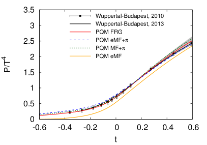
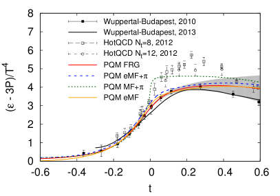
Figure 2: $(2+1)$-flavour FRG results for the pressure (left) and interaction measure (right) compared to the lattice, [16, 18, 19], and mean-field results. See text for details.

As discussed above, we have used the pressure to fix the open parameter $T_{\rm cr}^{\rm glue}$. This entails of course, that our results agree well with the lattice results at $t=0$. Away from $t=0$, on the other hand, the agreement can be attributed to the proper inclusion of the relevant dynamics. Especially our FRG result (red, solid curve) agrees very well with the lattice throughout the whole temperature range. This can be seen more clearly in the interaction measure, shown in the right panel of Fig. 2. Clearly, the MF result is too steep in the interaction region and its peak is too high as compared to the continuum extrapolated lattice result by the Wuppertal-Budapest collaboration (full symbols). The eMF result is still slightly to steep in the transition region. Finally, our FRG result lies almost on top of the lattice points. This coincidence is not only due to the presence of matter fluctuations. In fact, the inclusion of unquenching effects, $t_{\rm YM}(t_{\rm glue})$, results in a drastic reduction of the peak height in the interaction measure towards the lattice results, see also [2, 41] for a direct comparison in MF.

At high temperatures, our results start to deviate from the lattice. However, this is the region where the influence of the UV cutoff $\Lambda=1$ GeV sets in. Furthermore, Eq. (4) ceases to be valid at high scales where the slope saturates and the perturbative limit is reached. The grey band in Fig. 2 gives an estimate of the error in our FRG result. It is obtained from the change of the threshold functions with respect to the temperature, at vanishing mass at the ultraviolet cutoff $\Lambda$, see [1] for details.

6 Conclusions

In this talk we have discussed the inclusion of unquenching effects in the glue potential in QCD effective models. Recent first-principles continuum results for the unquenched glue potentials, [5, 6, 7, 27], have allowed to improve the glue sector of effective models significantly, which had thus far been badly constrained: mostly a Ginzburg–Landau-like ansatz for the glue potential, fitted to lattice Yang-Mills theory, had been used. In [2] it was shown that by a simple rescaling of the temperature in the standard Yang-Mills based Polyakov-loop potentials one can already capture the essential glue dynamics of the unquenched system. There, results in the mean-field approximation have been put forward. Here, we have taken the next step and included thermal and quantum fluctuations in the matter sector with the functional renormalisation group.

We have investigated order parameters and thermodynamic observables within the Polyakov-extended quark-meson model with $2+1$ flavours. This type of model can be systematically related to full QCD, as e.g. discussed in [2, 3, 9]. A comparison to lattice QCD simulations with $2~{}+~{}1$ flavours shows excellent agreement up to temperatures of approximately $1.3$ times the critical temperature. Therefore, we conclude that most of the relevant dynamics for the QCD crossover can already be captured within the PQM model.

The present work serves as a benchmark of our system at vanishing chemical potential, which allows us to conclude that we have all relevant fluctuations included. Since our approach is not restricted to the zero chemical potential region we can now aim at the full phase diagram, $\mu\geq 0$ .

- [1] T. K. Herbst, M. Mitter, J. M. Pawlowski, B.-J. Schaefer, and R. Stiele, “Thermodynamics of qcd at vanishing density,” arXiv:1308.3621 [hep-ph].
- [2] L. M. Haas, R. Stiele, J. Braun, J. M. Pawlowski, and J. Schaffner-Bielich, “Improved polyakov-loop potential for effective models from functional calculations,” Phys.Rev. D87 (Apr, 2013) 076004, arXiv:1302.1993 [hep-ph].
- [3] T. K. Herbst, J. M. Pawlowski, and B.-J. Schaefer, “On the phase structure and thermodynamics of qcd,” Phys. Rev. D88 (2013) 014007, arXiv:1302.1426 [hep-ph].
- [4] M. Mitter and B.-J. Schaefer, “Fluctuations and the axial anomaly with three quark flavors,” arXiv:1308.3176 [hep-ph].
- [5] J. Braun, H. Gies, and J. M. Pawlowski, “Quark confinement from color confinement,” Phys.Lett. B684 (2010) 262–267, arXiv:0708.2413 [hep-th].
- [6] J. Braun, L. M. Haas, F. Marhauser, and J. M. Pawlowski, “Phase structure of two-flavor qcd at finite chemical potential,” Phys.Rev.Lett. 106 (2011) 022002, arXiv:0908.0008 [hep-ph].
- [7] L. Fister and J. M. Pawlowski, “Confinement from correlation functions,” Phys.Rev. D88 (2013) 045010, arXiv:1301.4163 [hep-ph].
- [8] C. S. Fischer, L. Fister, J. Luecker, and J. M. Pawlowski, “Polyakov loop potential at finite density,” arXiv:1306.6022 [hep-ph].
- [9] J. M. Pawlowski, “The qcd phase diagram: Results and challenges,” AIP Conf.Proc. 1343 (2011) 75–80, arXiv:1012.5075 [hep-ph].
- [10] K. Fukushima, “Chiral effective model with the polyakov loop,” Phys.Lett. B591 (2004) 277–284, arXiv:hep-ph/0310121.
- [11] E. Megias, E. Ruiz Arriola, and L. Salcedo, “Polyakov loop in chiral quark models at finite temperature,” Phys.Rev. D74 (2006) 065005, arXiv:hep-ph/0412308.
- [12] C. Ratti, M. A. Thaler, and W. Weise, “Phases of qcd: Lattice thermodynamics and a field theoretical model,” Phys.Rev. D73 (2006) 014019, arXiv:hep-ph/0506234.
- [13] S. Mukherjee, M. G. Mustafa, and R. Ray, “Thermodynamics of the pnjl model with nonzero baryon and isospin chemical potentials,” Phys.Rev. D75 (2007) 094015, arXiv:hep-ph/0609249 [hep-ph].
- [14] B.-J. Schaefer, J. M. Pawlowski, and J. Wambach, “The phase structure of the polyakov–quark-meson model,” Phys.Rev. D76 (2007) 074023, arXiv:0704.3234 [hep-ph].
- [15] A. Bazavov, T. Bhattacharya, M. Cheng, C. DeTar, H. Ding, et al., “The chiral and deconfinement aspects of the qcd transition,” Phys.Rev. D85 (2012) 054503, arXiv:1111.1710 [hep-lat].
- [16] HotQCD Collaboration Collaboration, A. Bazavov, “The qcd equation of state with 2+1 flavors of highly improved staggered quarks (hisq),” Nucl.Phys. A904-905 (2013) 877c–880c, arXiv:1210.6312 [hep-lat].
- [17] Wuppertal-Budapest Collaboration Collaboration, S. Borsanyi et al., “Is there still any mystery in lattice qcd? results with physical masses in the continuum limit iii,” JHEP 1009 (2010) 073, arXiv:1005.3508 [hep-lat].
- [18] S. Borsanyi, G. Endrodi, Z. Fodor, A. Jakovac, S. D. Katz, et al., “The qcd equation of state with dynamical quarks,” JHEP 1011 (2010) 077, arXiv:1007.2580 [hep-lat].
- [19] S. Borsanyi, Z. Fodor, C. Hoelbling, S. D. Katz, S. Krieg, et al., “Full result for the qcd equation of state with 2+1 flavors,” arXiv:1309.5258 [hep-lat].
- [20] B.-J. Schaefer and M. Wagner, “The three-flavor chiral phase structure in hot and dense qcd matter,” Phys.Rev. D79 (2009) 014018, arXiv:0808.1491 [hep-ph].
- [21] T. K. Herbst, J. M. Pawlowski, and B.-J. Schaefer, “The phase structure of the polyakov–quark-meson model beyond mean field,” Phys.Lett. B696 (2011) 58–67, arXiv:1008.0081 [hep-ph].
- [22] B.-J. Schaefer and J. Wambach, “The phase diagram of the quark meson model,” Nucl.Phys. A757 (2005) 479–492, arXiv:nucl-th/0403039.
- [23] D. Jungnickel and C. Wetterich, “Effective action for the chiral quark-meson model,” Phys.Rev. D53 (1996) 5142–5175, arXiv:hep-ph/9505267.
- [24] G. ’t Hooft, “Computation of the quantum effects due to a four-dimensional pseudoparticle,” Phys.Rev. D14 (1976) 3432–3450.
- [25] G. ’t Hooft, “Symmetry breaking through bell-jackiw anomalies,” Phys.Rev.Lett. 37 (1976) 8–11.
- [26] B.-J. Schaefer and M. Mitter, “Three-flavor chiral phase transition and axial symmetry breaking with the functional renormalization group,” arXiv:1312.3850 [hep-ph].
- [27] J. Braun, A. Eichhorn, H. Gies, and J. M. Pawlowski, “On the nature of the phase transition in su(n), sp(2) and e(7) yang-mills theory,” Eur.Phys.J. C70 (2010) 689–702, arXiv:1007.2619 [hep-ph].
- [28] R. D. Pisarski, “Quark gluon plasma as a condensate of su(3) wilson lines,” Phys.Rev. D62 (2000) 111501, arXiv:hep-ph/0006205.
- [29] S. Roessner, C. Ratti, and W. Weise, “Polyakov loop, diquarks and the two-flavour phase diagram,” Phys.Rev. D75 (2007) 034007, arXiv:hep-ph/0609281.
- [30] K. Fukushima, “Phase diagrams in the three-flavor nambu-jona-lasinio model with the polyakov loop,” Phys.Rev. D77 (2008) 114028, arXiv:0803.3318 [hep-ph].
- [31] P. M. Lo, B. Friman, O. Kaczmarek, K. Redlich, and C. Sasaki, “Polyakov loop fluctuations in su(3) lattice gauge theory and an effective gluon potential,” Phys. Rev. D 88, 074502 (2013) , arXiv:1307.5958 [hep-lat].
- [32] N. Strodthoff, B.-J. Schaefer, and L. von Smekal, “Quark-meson-diquark model for two-color qcd,” Phys.Rev. D85 (2012) 074007, arXiv:1112.5401 [hep-ph].
- [33] B. W. Mintz, R. Stiele, R. O. Ramos, and J. Schaffner-Bielich, “Phase diagram and surface tension in the 3-flavor polyakov-quark-meson model,” Phys.Rev. D87 (2013) 036004, arXiv:1212.1184 [hep-ph].
- [34] V. Skokov, B. Friman, E. Nakano, K. Redlich, and B.-J. Schaefer, “Vacuum fluctuations and the thermodynamics of chiral models,” Phys.Rev. D82 (2010) 034029, arXiv:1005.3166 [hep-ph].
- [35] B.-J. Schaefer and M. Wagner, “Qcd critical region and higher moments for three flavor models,” Phys.Rev. D85 (2012) 034027, arXiv:1111.6871 [hep-ph].
- [36] H. Gies and C. Wetterich, “Renormalization flow of bound states,” Phys.Rev. D65 (2002) 065001, arXiv:hep-th/0107221.
- [37] H. Gies and C. Wetterich, “Universality of spontaneous chiral symmetry breaking in gauge theories,” Phys.Rev. D69 (2004) 025001, arXiv:hep-th/0209183 [hep-th].
- [38] J. M. Pawlowski, “Aspects of the functional renormalisation group,” Annals Phys. 322 (2007) 2831–2915, arXiv:hep-th/0512261.
- [39] S. Floerchinger and C. Wetterich, “Exact flow equation for composite operators,” Phys.Lett. B680 (2009) 371–376, arXiv:0905.0915 [hep-th].
- [40] F. Marhauser and J. M. Pawlowski, “Confinement in polyakov gauge,” arXiv:0812.1144 [hep-ph].
- [41] R. Stiele, L. M. Haas, J. Braun, J. M. Pawlowski, and J. Schaffner-Bielich, “Qcd thermodynamics of effective models with an improved polyakov-loop potential,” PoS ConfinementX (2012) 215, arXiv:1303.3742 [hep-ph].