Kinematic Properties of Slow ICMEs and an Interpretation of a Modified Drag Equation for Fast and Moderate ICMEs

Abstract

We report kinematic properties of slow interplanetary coronal mass ejections (ICMEs) identified by SOHO/LASCO, interplanetary scintillation, and in-situ observations, and propose a modified equation for the ICME motion. We identify seven ICMEs between 2010 and 2011, and examine them with 39 events reported in our previous work. We examine 15 fast ($V_{\mathrm{SOHO}}-V_{\mathrm{bg}}>500$ ${\mathrm{km~{}s^{-1}}}$), 25 moderate ($0$ $\mathrm{km~{}s^{-1}}$ $\leq V_{\mathrm{SOHO}}-V_{\mathrm{bg}}\leq 500$ ${\mathrm{km~{}s^{-1}}}$), and 6 slow ($V_{\mathrm{SOHO}}-V_{\mathrm{bg}}<$ $0$ ${\mathrm{km~{}s^{-1}}}$) ICMEs, where ${V_{\mathrm{SOHO}}}$ and ${V_{\mathrm{bg}}}$ are the initial speed of ICMEs and the speed of the background solar wind, respectively. For slow ICMEs, we found the following results: i) They accelerate toward the speed of the background solar wind during their propagation, and reach their final speed by ${0.34\pm 0.03}$ AU. ii) The acceleration ends when they reach $479\pm 126$ ${\mathrm{km~{}s^{-1}}}$; this is close to the typical speed of the solar wind during the period of this study. iii) When ${{\gamma}_{\mathrm{1}}}$ and ${{\gamma}_{\mathrm{2}}}$ are assumed to be constants, a quadratic equation for the acceleration $a=-{\gamma}_{\mathrm{2}}(V-V_{\mathrm{bg}})|V-V_{\mathrm{bg}}|$ is more appropriate than a linear one $a=-{\gamma}_{\mathrm{1}}(V-V_{\mathrm{bg}})$, where $V$ is the propagation speed of ICMEs, while the latter gives a smaller ${\chi}^{2}$ value than the former. For the motion of the fast and moderate ICMEs, we found a modified drag equation $a=-2.07{\times}10^{-12}(V-V_{\mathrm{bg}})|V-V_{\mathrm{bg}}|-4.84{\times}10^{-6}(V-V_{\mathrm{bg}})$. From the viewpoint of fluid dynamics, we interpret this equation as indicating that ICMEs with ${0}$ ${\mathrm{km~{}s^{-1}}}$ $\leq V-V_{\mathrm{bg}}\leq 2300$ ${\mathrm{km~{}s^{-1}}}$ are controlled mainly by the hydrodynamic Stokes drag force, while the aerodynamic drag force is a predominant factor for the propagation of ICME with $V-V_{\mathrm{bg}}>2300$ ${\mathrm{km~{}s^{-1}}}$.

1 Introduction

introduction

Coronal mass ejections (CMEs) are transient events in which a large amount of plasma and magnetic field are expelled from the Sun into the interplanetary space with a wide range of speed. Interplanetary coronal mass ejections (ICMEs) are defined as CMEs propagating far from the Sun [Howard (2011)]. Some of them reach the Earth and sometimes cause severe geomagnetic storms [Gosling et al. (1991), Brueckner et al. (1998), Cane, Richardson, and St. Cyr, O.C. (2000)]. Therefore, understanding of ICME propagation is very important for space weather forecasting. It is known that the range of ICME speeds in the near-Earth region is narrower than that in the near-Sun region by space-borne coronagraphs and near-Earth in-situ observations (e.g. Lindsay1999; Gopalswamy2000, 2001). On the basis of this fact, many investigators expect that ICMEs undergo an interaction with the ambient interplanetary medium. Vrsnak2002 proposed a model for the motion of ICMEs in which the interaction with the solar wind is simply expressed by the following equation for the acceleration:

$$\ilabel{eq.linear}a=-{\gamma}_{\mathrm{1}}(V-V_{\mathrm{bg}}),$$ (1)

where ${{\gamma}_{\mathrm{1}}}$ is a function of distance, and $V$ and $V_{\mathrm{bg}}$ are the speeds of ICMEs and of the background solar wind, respectively. They also compared their model with the drag acceleration of the following form:

$$\ilabel{eq.quadratic}a=-{\gamma}_{\mathrm{2}}(V-V_{\mathrm{bg}})|V-V_{\mathrm{bg}}|,$$ (2)

where ${{\gamma}_{\mathrm{2}}}$ is another function of distance; this expression is known as the aerodynamic drag force (e.g. Chen1996; Cargill2004; Vrsnak2010). Although the motion of ICMEs is also affected by the Lorentz and gravity forces in the near-Sun region, it is expected that both forces become negligible at a large distance Chen (1996). Therefore, they take only the effect of drag force into account. Borgazzi et al. (2008, 2009) studied the dynamics of ICMEs in the solar wind using the hydrodynamic theory. They introduced two kinds of drag force depending on $V-V_{\mathrm{bg}}$ (a laminar drag) and $(V-V_{\mathrm{bg}})^{2}$ (a turbulent drag) to the equation of motion.

Drag force models have been tested by comparing with ICME observations. Reiner2003 examined the speed profile of a CME obtained by measurements of type-II radio bursts. Tappin2006 studied the propagation of a CME that occurred on 5 April 2003 using observations by the Large Angle and Spectrometric Coronagraph (LASCO; Brueckner1995) onboard the Solar and Heliosphere Observatory (SOHO) spacecraft, Solar Mass Ejection Imager (SMEI) onboard the Coriolis satellite, and the Ulysses interplanetary probe. Manoharan2006 examined radial evolutions of 30 CMEs observed by SOHO/LASCO, Advanced Composition Explorer (ACE; Stone1998), and the Ooty radio telescope between 1998 and 2004. Maloney2010 derived three-dimensional kinematics of three ICMEs detected between 2008 and 2009 using the Sun Earth Connection Coronal and Heliospheric Investigation (SECCHI) instruments onboard the Solar-Terrestrial Relations Observatory (STEREO) A and B spacecraft. Temmer2011 also studied the influence of the solar wind on the propagation of three ICMEs using the same spacecraft. Lara2011 investigated the velocity profile of an ICME from the Sun to 5.3 AU using data from SOHO/LASCO, ACE, and Ulysses, and then estimated the drag coefficient and the kinematic viscosity for the ICME–solar wind interaction on the basis of fluid dynamics.

We assume that the radial motion of ICMEs is governed by the drag force(s) due to interaction with the background solar wind, and that the magnitude of the force is proportional to the difference in speed between the ICME and the solar wind. Our assumption should be tested using data obtained by interplanetary observations. We take advantage of the interplanetary scintillation (IPS; Hewish1964) observations to determine the speeds and accelerations of ICMEs. Our IPS observations have been carried out since early 1980s using the 327 MHz radio-telescope system of the Solar-Terrestrial Environment Laboratory (STEL), Nagoya University Kojima and Kakinuma (1990). These observations allow us to probe into the inner heliosphere with a cadence of 24 h, and therefore are suitable to collecting global data on ICMEs.

In our previous study (Iju2013; referred to as Paper I), we detected 39 ICMEs using the IPS observations by the Kiso IPS antenna Asai et al. (1995) during 1997 – 2009. Using the values of the initial speed ($V_{\mathrm{SOHO}}$) and $V_{\mathrm{bg}}$, we classified them into three types: fast ($V_{\mathrm{SOHO}}-V_{\mathrm{bg}}>500$ $\mathrm{km~{}s^{-1}}$), moderate ($0~{}{\mathrm{km~{}s^{-1}}}\leq V_{\mathrm{SOHO}}-V_{\mathrm{bg}}\leq 500$ ${\mathrm{km~{}s^{-1}}}$), and slow ($V_{\mathrm{SOHO}}-V_{\mathrm{bg}}<0$ $\mathrm{km~{}s^{-1}}$), and then examined their kinematic properties. From this examination, we found that fast and moderate ICMEs decelerate, while slow ones accelerate, and their radial speeds converge toward the speed of the solar wind as the distance increases. We also found that Equation (eq.linear) is more appropriate than (eq.quadratic) to describe the kinematics of ICMEs moving faster than the solar wind.

In the current study, we add new ICMEs identified between 2010 and 2011 to our list, and then examine their kinematics again on the assumption that ICMEs are controlled by the drag force(s) only. Earlier observational studies were mainly on the propagation of fast ICMEs, although the propagation of slow ICMEs was also studied (e.g. Shanmugaraju2009; Byrne2010; Maloney2010; Lynch2010; Temmer2011; Shen2011; Rollett2012; Vrsnak2013). These earlier studies presented mainly case studies of slow ICMEs. However, understanding the general properties of their propagation requires a statistical study. Hence, in this article we focus on the kinematics of slow ICMEs, and determine their general properties by statistical analysis. We also examine fast and moderate ICMEs in further detail. Although we showed a simple equation for their motion in Paper I, we will provide a modified one and its physical implications in this article.

The outline of this article is as follows. Section data and method describes IPS observations, methods for event identification, and estimating ICME speeds and accelerations. Section results provides the speed profiles of ICMEs and the analyses of the propagation properties. Section discussion discusses the propagation of slow ICMEs, a modified drag equation for fast and moderate ICMEs, and the estimated viscosity for the ICME–solar wind interaction. Section conclusion summarizes the main conclusions of our study.

2 Data and Analysis Method

data and method

The solar wind disturbance factor, the so called “g-value” Gapper et al. (1982), is derived from IPS observations, and represents the relative level of density fluctuation integrated along the line-of-sight (LOS) from an observed radio source to a telescope. When dense plasma passes across the LOS, the g-value becomes greater than unity, while that is about unity for the quiet solar wind. In the current study, we use g-value data obtained between 2010 and 2011. The measurement of g-value has been carried out using the Solar Wind Imaging Facility (SWIFT; Tokumaru2011) since 2010. From an examination of these data, we found 260 disturbance days between 2010 and 2011, and made a list of them.

These disturbance days should be compared with CME/ICME pairs identified using SOHO/LASCO and in-situ observations. In this examination, because there was no list of CME/ICME pairs between 2010 and 2011, we identified them ourselves using the SOHO/LASCO CME catalog (Yashiro2004; Gopalswamy2009; available at cdaw.gsfc.nasa.gov/CME˙list/), 1 and 2 h averaged data of solar-wind charge states obtained by the Solar Wind Ion Composition Spectrometer (SWICS; Gloeckler1998) onboard ACE (available at www.srl.caltech.edu/ACE/ASC/), and the criteria of ICME identification introduced by Richardson2010. According to the above paper, the mean Fe charge ${\langle\mathrm{Q}_{\mathrm{Fe}}\rangle}$ and O viii / O vii ratio are enhanced during the passage of an ICME. Hence, we define the detection of a near-Earth ICME as the enhancement in the charge state observed by ACE/SWICS within five days after the appearance of a major Earth-side CME in the SOHO/LASCO-C2 field-of-view (FOV). The start and end times of an ICME event correspond to those of the charge-state enhancement, respectively. Using the above method, we made a list of CME/ICMEs found between 2010 and 2011.

We compared the list of disturbance days with that of CME/ICMEs by assuming that an ICME causes a disturbance day. We then identified seven ICMEs that were detected by SOHO/LASCO, IPS, and in-situ observations between 2010 and 2011. For them, we calculated the average reference distances (${R_{\mathrm{1}}}$ and ${R_{\mathrm{2}}}$), the average radial speeds (${V_{\mathrm{1}}}$ and ${V_{\mathrm{2}}}$), and accelerations (${a_{\mathrm{1}}}$ and ${a_{\mathrm{2}}}$). We also estimated the transit speed (${V_{\mathrm{Tr}}}$) using the appearance time in the SOHO/LASCO-C2 FOV (${T_{\mathrm{SOHO}}}$) and the detection time at 1 AU (${T_{\mathrm{Earth}}}$). The initial speed of the associated CMEs (${V_{\mathrm{SOHO}}}$) was estimated from their speed measured in the plane of the sky by SOHO/LASCO (${V_{\mathrm{POS}}}$). The radial speed of near-Earth ICMEs (${V_{\mathrm{Earth}}}$) is equivalent to the speed of plasma flow during the charge-state enhancement derived from in-situ measurements. We note that ${V_{\mathrm{SOHO}}}$ and ${V_{\mathrm{Earth}}}$ represent the average values in the near-Sun and near-Earth regions. Linkewise, ${V_{\mathrm{1}}}$ and ${a_{\mathrm{1}}}$ are averages in the SOHO–IPS region (from 0.1 to ${\approx}$ 0.6 AU), and ${V_{\mathrm{2}}}$ and ${a_{\mathrm{2}}}$ are averages in the IPS–Earth region (from ${\approx}$ 0.6 to 1 AU). To determine the speed of the background solar wind ${V_{\mathrm{bg}}}$, we used the OMNI dataset through OMNIWeb Plus (omniweb.gsfc.nasa.gov/). Using the value of ${V_{\mathrm{SOHO}}}$ and ${V_{\mathrm{bg}}}$, we have classified seven ICMEs into fast ($V_{\mathrm{SOHO}}-V_{\mathrm{bg}}>500$ ${\mathrm{km~{}s^{-1}}}$), moderate ($0$ ${\mathrm{km~{}s^{-1}}}$ $\leq V_{\mathrm{SOHO}}-V_{\mathrm{bg}}\leq 500$ ${\mathrm{km~{}s^{-1}}}$), and slow ($V_{\mathrm{SOHO}}-V_{\mathrm{bg}}<$ $0$ ${\mathrm{km~{}s^{-1}}}$) ones. In our results, the numbers of fast, moderate, and slow ICMEs are 1, 5, and 1, respectively. Detailed methods of calculation for the above properties were presented in Paper I.

3 Results

results

We list the properties of seven ICMEs detected by SWIFT between 2010 and 2011 in Tables table1 and table2 including ${R_{\mathrm{0}}}$, ${T_{\mathrm{IPS}}}$, ${\alpha}$, and ${\beta}$ in addition to ${T_{\mathrm{SOHO}}}$, ${V_{\mathrm{POS}}}$, ${V_{\mathrm{SOHO}}}$, ${R_{\mathrm{1}}}$, ${V_{\mathrm{1}}}$, ${a_{\mathrm{1}}}$, ${R_{\mathrm{2}}}$, ${V_{\mathrm{2}}}$, ${a_{\mathrm{2}}}$, ${T_{\mathrm{Earth}}}$, ${V_{\mathrm{Earth}}}$, ${V_{\mathrm{Tr}}}$, and ${V_{\mathrm{bg}}}$. Here, ${T_{\mathrm{IPS}}}$ and ${R_{\mathrm{0}}}$ are the mean detection time and average radial distance for a disturbance detected by IPS observations, respectively; their detailed descriptions were presented in Paper I. Parameters ${\alpha}$ and ${\beta}$ are defined as

$$\ilabel{eq.powerlaw}V={\beta}R^{\alpha},$$ (3)

where $R$ is the heliocentric distance. On the other hand, the catalog of 39 ICMEs detected by the Kiso IPS antenna during 1997 – 2009 was given in Paper I. We also provide a list of slow ICMEs extracted from the above catalog in Tables table3 and table4. Therefore, we examine 46 ICMEs which consist of 15 fast, 25 moderate, and 6 slow ones identified during 1997 – 2011. In this investigation, we assume that ${V_{\mathrm{bg}}}$ is constant for heliocentric distances ranging from ${\approx}$ 0.1 to 1 AU. This assumption is consistent with the speed profile of the solar wind estimated using coronagraph observations Sheeley et al. (1997); Guhathakurta and Fisher (1998). The constant speed of the solar wind has been verified between ${\approx}$ 0.3 and 1 AU by in-situ measurements Schwenn et al. (1981). =17.2cm

Properties derived from SOHO/LASCO, IPS (SWIFT), and in-situ observations for seven ICMEs during 2010 – 2011. table1 SOHO/LASCO IPS Disturbance SOHO–IPS region Date Time ${V_{\mathrm{POS}}}$ ${V_{\mathrm{SOHO}}}$ CME PA Date Time ${R_{\mathrm{0}}}$ [AU] $R_{\mathrm{1}}$ [AU] $V_{\mathrm{1}}$ [$\mathrm{km~{}s^{-1}}$] $a_{\mathrm{1}}$ [$\mathrm{m~{}s^{-2}}$] No. [ddmmmyyyy] [hhmm] [${\mathrm{km~{}s^{-1}}}$] [${\mathrm{km~{}s^{-1}}}$] Type [deg] [ddmmmyyyy] [hhmm] aver. ${\sigma}$ aver. ${\sigma}$ aver. ${\sigma}$ aver. ${\sigma}$ 1 07 Feb 2010 0354 421  505 FH $-99$ 11 Feb 2010 0117 0.81 0.20 0.45 0.10  359  92 $-0.44$ 0.56 2 03 Apr 2010 1033 668  802 FH $-99$ 04 Apr 2010 0043 0.81 0.16 0.44 0.08 1030 236 $-0.77$ 1.56 3 08 Apr 2010 0131 227  272 PH $~{}76$ 11 Apr 2010 0240 0.67 0.22 0.37 0.11  374 122 $~{}0.90$ 0.84 4 24 May 2010 1406 427  512 FH $-99$ 26 May 2010 0251 0.63 0.19 0.35 0.09  466 135 $-0.51$ 0.53 5 01 Aug 2010 1342 850 1020 FH $-99$ 03 Aug 2010 0356 0.77 0.21 0.43 0.11  563 160 $-1.70$ 1.67 6 12 Nov 2010 0836 482  578 PH $170$ 15 Nov 2010 0201 0.80 0.16 0.44 0.08  501 105 $-0.56$ 0.65 7 15 Feb 2011 0224 669  803 FH $-99$ 17 Feb 2011 0307 0.73 0.17 0.41 0.08  615 135 $-1.49$ 0.87 Column: (1) Event number; (2) – (3) Appearance date [ddmmmyyyy] and time [hhmm] of an ICME–associated CME observed by SOHO/LASCO;(4) Speed in the sky plane measured by SOHO/LASCO at a reference distance of 0.08 AU; (5) Radial speed estimated using $V_{\mathrm{SOHO}}=1.20\times V_{\mathrm{POS}}$; (6) Type of CME (FH, PH, and NM mean Full Halo, Partial Halo, and Normal CME, respectively); (7) Position angle measured counter-clockwise from solar north in degrees ($-99$ means Full Halo); (8) – (9) Observation date [ddmmmyyyy] and mean time [hhmm] of IPS disturbance event day ; (10) – (11) Average and standard errors for the distance of observed disturbance ${R_{\mathrm{0}}}$; (12) – (13) Average and standard errors for the reference distance ${R_{\mathrm{1}}}$ in the SOHO–IPS region; (14) – (15) Average and standard errors for the speed ${V_{\mathrm{1}}}$ in the SOHO–IPS region; (16) – (17) Average and standard errors for acceleration ${a_{\mathrm{1}}}$ in the SOHO–IPS region.

=17.2cm

Properties derived from SOHO/LASCO, IPS (SWIFT), and in-situ observations for seven ICMEs, and speeds of the background solar wind during 2010 – 2011. table2 IPS in situ Parameters for IPS–Earth region power-law equation                Background wind $R_{\mathrm{2}}$ [AU] $V_{\mathrm{2}}$ [$\mathrm{km~{}s^{-1}}$] $a_{\mathrm{2}}$ [$\mathrm{m~{}s^{-2}}$] Date Time $V_{\mathrm{Earth}}$ Index Coefficient $V_{\mathrm{Tr}}$  $V_{\mathrm{bg}}$ [$\mathrm{km~{}s^{-1}}$] No. aver. ${\sigma}$ aver. ${\sigma}$ aver. ${\sigma}$ [ddmmmyyyy] [hhmm] [$\mathrm{km~{}s^{-1}}$] ${\alpha}$ ${\beta}$ [$\mathrm{km~{}s^{-1}}$] aver. $\sigma$ 1 0.91 0.10 356 376 $~{}0.62$ 2.29 12 Feb 2010 0000 410 $-0.113$ 366.1 358 339 23 2 0.90 0.07 388 300 $~{}0.01$ 2.40 05 Apr 2010 1600 701 $-0.160$ 599.7 776 540 90 3 0.83 0.11 640 445 $-1.10$ 2.89 12 Apr 2010 0000 419  $0.255$ 514.2 439 461 74 4 0.81 0.09 359 175 $-0.25$ 0.68 28 Apr 2010 1600 373 $-0.140$ 370.3 424 328 22 5 0.89 0.10 786 692 $-1.62$ 7.97 04 Aug 2010 1000 592 $-0.169$ 620.4 608 461 35 6 0.90 0.08 395 303 $~{}1.46$ 1.94 16 Nov 2010 1800 557 $-0.080$ 468.7 476 534 72 7 0.87 0.08 466 298 $-0.38$ 1.78 18 Feb 2011 0300 506 $-0.203$ 487.3 572 534 46 Column: (1) Event number [identical with column (1) in Table table1]; (2) – (3) Average and standard errors for the reference distance $R_{\mathrm{2}}$ in the IPS–Earth region; (4) – (5) Average and standard errors for the speed $V_{\mathrm{2}}$ in the IPS–Earth region; (6) – (7) Average and standard errors for the acceleration $a_{\mathrm{2}}$ in the IPS–Earth region; (8) – (9) Detection date [ddmmmyyyy] and time [hhmm] of a near-Earth ICME by in-situ observation at 1 AU; (10) Near-Earth ICME speed measured by in-situ observation at 1 AU; (11) – (12); Index $\alpha$ and coefficient $\beta$ for a power-law form of radial speed evolution; (13) 1 AU transit speed derived from the CME appearance and the ICME detection times; (14) – (15) Average and standard errors for the speed of the background wind $V_{\mathrm{bg}}$ measured by spacecraft.

=17.2cm

Properties derived from SOHO/LASCO, IPS (KIT and SWIFT), and in-situ observations for six slow ICMEs during 1997 – 2011. table3 SOHO/LASCO IPS Disturbance SOHO–IPS region Date Time ${V_{\mathrm{POS}}}$ ${V_{\mathrm{SOHO}}}$ CME PA Date Time ${R_{\mathrm{0}}}$ [AU] ${R_{\mathrm{1}}}$ [AU] ${V_{\mathrm{1}}}$ [${\mathrm{km~{}s^{-1}}}$] ${a_{\mathrm{1}}}$ [${\mathrm{m~{}s^{-2}}}$] No. [ddmmmyyyy] [hhmm] [${\mathrm{km~{}s^{-1}}}$] [${\mathrm{km~{}s^{-1}}}$] Type [deg] [ddmmmyyyy] [hhmm] aver. ${\sigma}$ aver. ${\sigma}$ aver. ${\sigma}$ aver. ${\sigma}$ 1 13 Apr 1999 0330 291 349 PH $228$ 15 Apr 1999 0453 0.55 0.16 0.32 0.08  456 130 $~{}0.71$ 0.55 2 06 Aug 2000 1830 233 280 PH $105$ 09 Aug 2000 0503 0.62 0.14 0.35 0.07  432  95 $~{}0.68$ 0.40 3 14 Aug 2003 2006 378 454 FH $-99$ 17 Aug 2003 0409 0.68 0.12 0.38 0.06  497 106 $~{}0.62$ 0.63 4 12 Sep 2008 1030  91  91 NM $~{}89$ 14 Sep 2008 0449 0.58 0.10 0.33 0.05  556  96 $~{}2.04$ 0.34 5 29 May 2009 0930 139 139 NM $258$ 01 Jun 2009 0148 0.56 0.18 0.32 0.09  353 116 $~{}0.72$ 0.32 6 08 Apr 2010 0131 227 272 PH $~{}76$ 11 Apr 2010 0240 0.67 0.22 0.37 0.11  374 122 $~{}0.90$ 0.84 Column: (1) Event number; (2) – (3) Appearance date [ddmmmyyyy] and time [hhmm] of an ICME–associated CME observed by SOHO/LASCO;(4) Speed in the sky plane measured by SOHO/LASCO at a reference distance of 0.08 AU ; (5) Radial speed estimated using $V_{\mathrm{SOHO}}=1.20\times V_{\mathrm{POS}}$; (6) Type of CME (FH, PH, and NM mean Full Halo, Partial Halo, and Normal CME, respectively); (7) Position angle measured counter-clockwise from solar north in degrees ($-99$ means Full Halo); (8) – (9) Observation date [ddmmmyyyy] and mean time [hhmm] of IPS disturbance event day ; (10) – (11) Average and standard errors for the distance of observed disturbance ${R_{\mathrm{0}}}$; (12) – (13) Average and standard errors for the reference distance ${R_{1}}$ in the SOHO–IPS region; (14) – (15) Average and standard errors for the speed ${V_{\mathrm{1}}}$ in the SOHO–IPS region; (16) – (17) Average and standard errors for acceleration ${a_{\mathrm{1}}}$ in the SOHO–IPS region.

=17.2cm

Properties derived from SOHO/LASCO, IPS (KIT and SWIFT), and in-situ observations for six slow ICMEs, and speeds of background solar wind during 1997–2011. table4 IPS in situ Parameters for IPS–Earth region power-law equation                Background wind $R_{\mathrm{2}}$ [AU] $V_{\mathrm{2}}$ [$\mathrm{km~{}s^{-1}}$] $a_{\mathrm{2}}$ [$\mathrm{m~{}s^{-2}}$] Date Time $V_{\mathrm{Earth}}$ Index Coefficient $V_{\mathrm{Tr}}$  $V_{\mathrm{bg}}$ [$\mathrm{km~{}s^{-1}}$] No. aver. ${\sigma}$ aver. ${\sigma}$ aver. ${\sigma}$ [ddmmmyyyy] [hhmm] [$\mathrm{km~{}s^{-1}}$] ${\alpha}$ ${\beta}$ [$\mathrm{km~{}s^{-1}}$] aver. $\sigma$ 1 0.78 0.08 495 165 $-0.49$ 0.73 16 Apr 1999 1800 410 $0.094$ 465.0 480 398  15 2 0.81 0.07 414 149 $~{}0.06$ 0.62 10 Aug 2000 1900 430 $0.165$ 447.8 430 412  36 3 0.84 0.06 666 265 $-1.84$ 1.70 18 Aug 2003 0100 450 $0.068$ 543.0 540 534  55 4 0.79 0.05 247  58 $-0.01$ 0.20 17 Sep 2008 0400 400 $0.486$ 425.8 366 406 107 5 0.78 0.09 256 103 $~{}0.02$ 0.28 04 Jun 2009 0200 310 $0.276$ 327.7 304 327  26 6 0.83 0.11 640 445 $-1.10$ 2.89 12 Apr 2010 0000 419 $0.255$ 514.2 439 461  74 Column: (1) Event number [identical with column (1) in Table table1]; (2) – (3) Average and standard errors for the reference distance $R_{\mathrm{2}}$ in the IPS–Earth region; (4) – (5) Average and standard errors for the speed $V_{\mathrm{2}}$ in the IPS–Earth region; (6) – (7) Average and standard errors for the acceleration $a_{\mathrm{2}}$ in the IPS–Earth region; (8) – (9) Detection date [ddmmmyyyy] and time [hhmm] of a near-Earth ICME by in-situ observation at 1 AU; (10) Near-Earth ICME speed measured by in-situ observation at 1 AU; (11) – (12); Index $\alpha$ and coefficient $\beta$ for a power-law form of radial speed evolution; (13) 1 AU transit speed derived from the CME appearance and the ICME detection times; (14) – (15) Average and standard errors for the speed of the background wind $V_{\mathrm{bg}}$ measured by spacecraft.

In the following figures, an error bar represents one standard deviation ($1\sigma$ error) of the mean for each parameter. Figure fig1 shows speed profiles for six slow ICMEs identified in this study. As shown here, the ICME speeds increase with the radial distance, and those at 1 AU are close to the speed of the solar wind for all of them. From this, we claim that their speed profiles are well fit by a power-law function within the error bars, excluding the 12 September 2008 event (see No.4 in Tables 3 and 4). The 12 September 2008 event has the largest difference in speed ($V_{\mathrm{SOHO}}-V_{\mathrm{bg}}=-314$ ${\mathrm{km~{}s^{-1}}}$) in our sample, while the others have $V_{\mathrm{SOHO}}-V_{\mathrm{bg}}>-200$ ${\mathrm{km~{}s^{-1}}}$.

Figure fig2 exhibits the relationship between the initial speed $V_{\mathrm{SOHO}}$ and the index ${\alpha}$ for slow ICMEs. As shown here, ${\alpha}$ decreases from $0.486$ to $0.068$ as ${V_{\mathrm{SOHO}}}$ increases. The intersection point between the best-fit line $\alpha=k_{\mathrm{1}}+k_{\mathrm{2}}V_{\mathrm{SOHO}}$ and the ${\alpha=0}$ line is designated as ${V_{\mathrm{c}}}$ in the following. Manoharan2006 studied the same relationship for 30 CMEs. Four of them are slow CMEs, which have a slower initial speed than the final. In order to compare with our result, they are also plotted in Figure fig2. We find that their values of ${\alpha}$ range from $0.58$ to $-0.06$. The mean values of ${V_{\mathrm{c}}}$ and coefficients ${k_{\mathrm{1}}}$ and ${k_{\mathrm{2}}}$ for the best-fit line, and their standard ($1\sigma$) errors are given in Table tablebestfit. From the above examination, we find $V_{\mathrm{c}}=479\pm 126$ ${\mathrm{km~{}s^{-1}}}$ as the threshold speed when ${\alpha}$ becomes zero, i.e. the slow ICMEs have zero acceleration.

In Figure fig3, we plot all of their speed profiles in order to compare radial-speed evolutions of slow ICMEs. Here, data points for each ICME are connected by solid lines instead of fitting by Equation (eq.powerlaw). We note that differences in speed (${V-V_{\mathrm{bg}}}$) are used instead of ICME speeds in the $y$-axis, which correspond to $V_{\mathrm{SOHO}}-V_{\mathrm{bg}}$ in the near-Sun region, $V_{\mathrm{1}}-V_{\mathrm{bg}}$ in the SOHO–IPS region, $V_{\mathrm{2}}-V_{\mathrm{bg}}$ in the IPS–Earth region, and $V_{\mathrm{Earth}}-V_{\mathrm{bg}}$ in the near-Earth region. From the top panel, we find that the speed differences range from ${-314}$ ${\mathrm{km~{}s^{-1}}}$ to ${-49}$ ${\mathrm{km~{}s^{-1}}}$ in the near-Sun region, while they show a narrow range from ${-84}$ ${\mathrm{km~{}s^{-1}}}$ to ${11}$ ${\mathrm{km~{}s^{-1}}}$ in the near-Earth region. The bottom panel shows the averaged profile for their propagation. Table tablespeedevolution gives the average values of the distance and of the speed difference with the standard error in each region for the slow ICMEs.

We attempt to show which of Equations (eq.linear) and (eq.quadratic) is more suitable to describe the relationship between the acceleration and the difference in speeds for slow ICMEs. We assume that ${{\gamma}_{\mathrm{1}}}$ and ${{\gamma}_{\mathrm{2}}}$ are constants because we want as few variables as possible to describe the relationship as Paper I.

            (a)                                               (b)

 

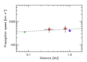
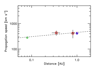
            (c)                                               (d)

 

            (e)                                               (f)

 

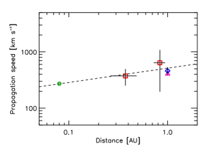
Figure 1.: Speed profiles for six slow ICMEs detected between (a) 13 and 16 April 1999, (b) 6 and 10 August 2000, (c) 14 and 18 August 2003, (d) 12 and 17 September 2008, (e)29 May and 4 June 2009, and (f) 8 and 12 April 2010. In each panel, the circle (green, at 0.08 AU), squares (red, at ${R_{\mathrm{1}}}$ and ${R_{\mathrm{2}}}$), and triangle (purple, at 1 AU) denote measurements of ICME speeds from SOHO/LASCO, IPS, and in-situ observations, respectively. Diamonds (blue, at 1 AU) indicate the speed of the background solar wind measured by in-situ observations, and the dashed line represents the power-law fit to the data using Equation (eq.powerlaw). fig1

Figure 2.: Relationship between the estimated initial speed ${V_{\mathrm{SOHO}}}$ and the index ${\alpha}$ [Equation (eq.powerlaw)] for six slow ICMEs. Circles show our data points, and crosses indicate those for the four slow events studied by Manoharan (2006). The solid and dotted lines denote the best-fit line $\alpha=k_{\mathrm{1}}+k_{\mathrm{2}}V_{\mathrm{SOHO}}$ and the $\alpha=0$ line, respectively. The arrow indicates the intersection of these two lines corresponding to the zero-acceleration point, $V_{\mathrm{c}}=479\pm 126$ ${\mathrm{km~{}s^{-1}}}$. fig2

                        (a)

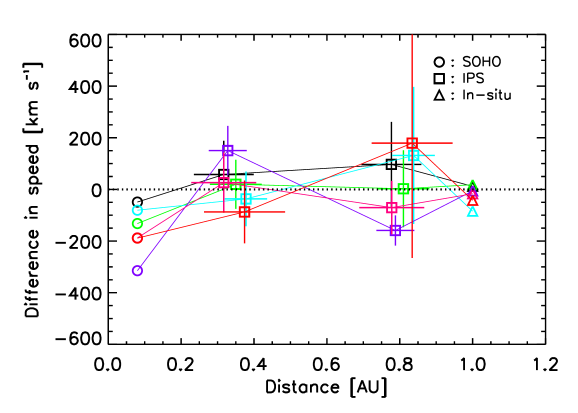
                       (b)

Figure 3.: Radial evolution of (a) differences in speed ($V-V_{\mathrm{bg}}$) for six slow ICMEs and (b) their averaged profiles. Circles, squares, and triangles indicate the values of ${V-V_{\mathrm{bg}}}$ for the ICMEs in near-Sun, interplanetary space, and near-Earth regions, respectively. Symbols for each ICME in panel (a) are connected by solid lines with the same color. The dotted line denotes the $V-V_{\mathrm{bg}}=0$ line in each panel. fig3

                      (a)

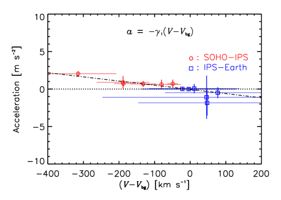
                     (b)

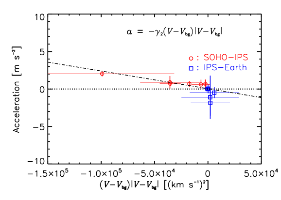
Figure 4.: Relationships between (a) acceleration ($a$) and difference in speed (${V-V_{\mathrm{bg}}}$) and (b) between $a$ and ${(V-V_{\mathrm{bg}})|V-V_{\mathrm{bg}}|}$ for six slow ICMEs in this study. Circles (red) and squares (blue) denote data points in the SOHO–IPS and IPS–Earth regions, respectively. The dash–dotted line and the dotted line denote the best-fit line and the zero-acceleration line, respectively, in each panel. fig4

                      (a)

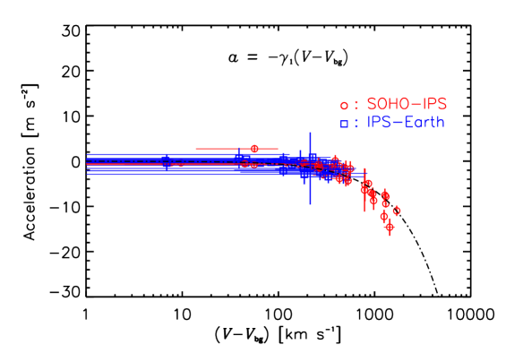
                      (b)

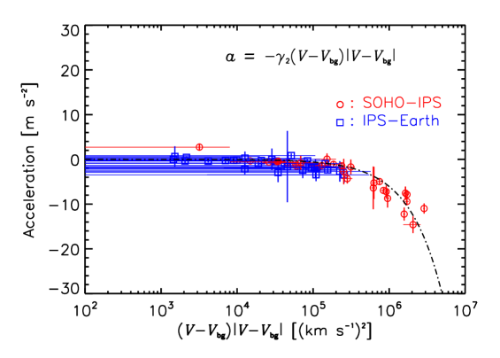
Figure 5.: Relationships between (a) acceleration ($a$) and difference in speed (${V-V_{\mathrm{bg}}}$) and (b) between $a$ and ${(V-V_{\mathrm{bg}})|V-V_{\mathrm{bg}}|}$ for 40 fast and moderate ICMEs (i.e. $V_{\mathrm{SOHO}}-V_{\mathrm{bg}}\geq 0$ ${\mathrm{km~{}s^{-1}}}$) in this study. Circles (red) and squares (blue) denote data points in the SOHO–IPS and IPS–Earth regions, respectively. The dash–dotted line shows the best-fit line in each panel. fig5

In Figure fig4, the top panel shows the relationship between $a$ and $V-V_{\mathrm{bg}}$, and the bottom panel between $a$ and $(V-V_{\mathrm{bg}})|V-V_{\mathrm{bg}}|$ for slow ICMEs. Data of ${V_{\mathrm{SOHO}}}$ and ${a_{\mathrm{1}}}$ were used for the SOHO–IPS region, while those of ${V_{\mathrm{IPS}}}$ and ${a_{\mathrm{2}}}$ were used for the IPS–Earth region. As shown here, the ${\chi}^{2}$ value for the linear equation is smaller than for the quadratic one. In Figure fig5, the top panel shows the relationship between $a$ and $V-V_{\mathrm{bg}}$, and the bottom panel between $a$ and $(V-V_{\mathrm{bg}})|V-V_{\mathrm{bg}}|$ for a group of fast and moderate ICMEs. Data of ${V_{\mathrm{SOHO}}}$ and ${a_{\mathrm{1}}}$ were used for the SOHO–IPS region, while those of ${V_{\mathrm{IPS}}}$ and ${a_{\mathrm{2}}}$ were used for the IPS–Earth region. In this figure, the best fit curves are not straight lines because of the logarithmic ${x}$-axis scale.

We derived the values of coefficients from the slopes of best-fit lines in Figures fig4 and fig5, and also calculated the reduced ${\chi}^{2}$ values in order to assess the goodness of fit. They are listed in Table tablecoef.

Table 1.: Mean values of the distance and of the speed difference with a standard error in each region for the slow ICMEs. tablespeedevolution

	Distance	Difference in speed
Region	[AU]	[${\mathrm{km~{}s^{-1}}}$]
Near-Sun	${0.08}$	${-159\pm 95}$
SOHO–IPS	${0.34\pm 0.08}$	${22\pm 111}$
IPS–Earth	${0.80\pm 0.08}$	${30\pm 197}$
Near-Earth	${1.00}$	${-20\pm 38}$

Table 2.: Mean values of coefficients ${k_{\mathrm{1}}}$ and ${k_{\mathrm{2}}}$ for the best-fit line ${\alpha=k_{\mathrm{1}}+k_{\mathrm{2}}V_{\mathrm{SOHO}}}$, the speed at the zero-acceleration point (${V_{\mathrm{c}}}$), and their standard errors. tablebestfit

	${k_{\mathrm{1}}}$	${k_{\mathrm{2}}}$	${V_{\mathrm{c}}}$ [${\mathrm{km~{}s^{-1}}}$]
Mean	${5.00\times 10^{-1}}$	${-1.04\times 10^{-3}}$	479
Standard error	${6.82\times 10^{-2}}$	${2.34\times 10^{-4}}$	126

Table 3.: Coefficients ${\gamma_{\mathrm{1}}}$, ${\gamma_{\mathrm{2}}}$, and reduced $\chi^{2}$ values for the slow ICMEs and a group of moderate and fast ones. tablecoef

Type of ICMEs	Coefficient
and equation	(Mean and standard error)	$\chi^{2}$
Slow ICMEs
Linear	${{\gamma}_{\mathrm{1}}=5.58(\pm 1.77)\times 10^{-6}}$ [${\mathrm{s^{-1}}}$]	0.24
Quadratic	${{\gamma}_{\mathrm{2}}=2.36(\pm 1.03)\times 10^{-11}}$ [${\mathrm{m^{-1}}}$]	0.36
Fast and Moderate ICMEs
Linear	${{\gamma}_{\mathrm{1}}=6.51(\pm 0.23)\times 10^{-6}}$ [${\mathrm{s^{-1}}}$]	1.14
Quadratic	${{\gamma}_{\mathrm{2}}=6.06(\pm 0.23)\times 10^{-12}}$ [${\mathrm{m^{-1}}}$]	2.50

4 Discussion

discussion

4.1 Kinematics of Slow ICMEs

slowICMEs

From Figure fig1, we confirm that all of the slow ICMEs accelerate toward the speed of the background solar wind during their outward propagation. Figure fig2 shows that the value of ${\alpha}$ decreases from 0.486 to 0.068 as the wind speed increases, up to the intersection point ${V_{\mathrm{c}}}$ where ${\alpha=0}$. Our range of ${\alpha}$ is consistent with that reported by Manoharan2006 for slow CMEs. As presented in Table tablebestfit, we derive the coefficients for the best-fit line and the value of ${V_{\mathrm{c}}}$ from the observational data. We find that our result ($\alpha=0.50-0.0010V_{\mathrm{SOHO}}$) is similar to $\alpha=0.69-0.0012V$ reported by Shanmugaraju2009 for the best-fit line. We note that their result was obtained from SOHO/LASCO observations with FOV $<32$ solar radii, while we studied the radial evolution of ICMEs in a wider region from the Sun to the Earth. The similarity between these best-fit lines implies that slow ICMEs quickly adjust to the speed of the solar wind. We also obtain $V_{\mathrm{c}}=479\pm 126$ ${\mathrm{km~{}s^{-1}}}$ as the threshold speed where ${\alpha}$ becomes zero, which is consistent with Paper I. The mean value is somewhat lower than the threshold speed of $575$ ${\mathrm{km~{}s^{-1}}}$ derived from their best-fit equation, though the difference is within the standard error.

Figure fig3 (a) shows that the distribution of speed differences in the near-Sun region is wider than in the near-Earth region. This and the above results justify our assumption that the motion of ICMEs is controlled by the drag force(s) due to interaction with the background solar wind. Temmer2011, Rollett2012, and Vrsnak2013 reported that the acceleration of slow ICMEs attains the speed of the solar wind within 0.5 AU. Figure fig3 (b) and Table tablespeedevolution show that the slow ICMEs attain their final speed by $0.34\pm 0.03$ AU. These are consistent with the earlier studies. It is emphasized that the acceleration cessation distance of ${\approx 0.3}$ AU for slow ICMEs is different from ${\approx 0.8}$ AU for fast ones as reported by Gopalswamy2001 and Paper I. Using the numerical MHD simulation, Vrsnak2010 found that ICMEs having a large angular width adjust to the speed of the solar wind already close to the Sun.

We confirm that not only a group of fast and moderate ICMEs, but also slow ICMEs show that the ${\chi}^{2}$ value for the linear equation is smaller than for the quadratic one. However, the assessment of significance level shows that Equation (eq.quadratic) is more suitable than (eq.linear) to describe the relationship between $a$ and $V-V_{\mathrm{bg}}$ for the slow ICMEs because the latter is too good to fit with data points. Maloney2010 introduced an equation of motion ${\mathrm{d}}V/{\mathrm{d}}t=-{\kappa}R^{-{\lambda}}(V-V_{\mathrm{bg}})^{\phi}$ in order to describe the motion of ICMEs, where ${\kappa}$, ${\lambda}$, and ${\phi}$ are constants. They reported that a quadratic equation ${({\phi}=2)}$ explained the motion of a slow ICME, while a linear equation ${({\phi}=1)}$ gave a better fitting than the quadratic one for the motion of a fast ICME. Byrne2010 also presented evidence that the aerodynamic drag force acted on a slow ICME of 12 December 2008. Our results are consistent with their studies for slow ICMEs. However, six events of slow ICMEs in our sample are not sufficient to investigate their kinematics more precisely, while we detected 40 events of fast and moderate ones during 1997 – 2011. We need to identify more slow ICMEs and then examine their propagation carefully.

4.2 Modified Drag Equation for Fast and Moderate ICMEs

modified equation

For the group of fast and moderate ICMEs, we find the values of coefficients ${\gamma}_{\mathrm{1}}$ and ${\gamma}_{\mathrm{2}}$, which are consistent with Paper I. Although the constancy of these coefficients is assumed in Equations (eq.linear) and (eq.quadratic), we also find a speed dependence in ${{\gamma}_{\mathrm{1}}}$ and ${{\gamma}_{\mathrm{2}}}$ as shown in Table tablecoef. In Paper I, we showed a linear relationship between the acceleration and difference in speed for a group of fast and moderate ICMEs, and then proposed a simple expression:

$$\ilabel{eq.previous}a=-6.58\times 10^{-6}(V-V_{\mathrm{bg}}),$$ (4)

as an equation of ICME motion on the assumption that the coefficient is constant in a speed range of $V_{\mathrm{SOHO}}-V_{\mathrm{bg}}\geq 0~{}{\mathrm{km~{}s^{-1}}}$. Now, we need to correct our assumption for the constancy of ${{\gamma}_{\mathrm{1}}}$.

In order to analyze this point in detail, we calculated the mean values of ${{\gamma}_{\mathrm{1}}}$ and difference in speed with the standard ($1\sigma$) error for each classification of ICMEs. These values are presented in Table table8. In this analysis, slow ICMEs are excluded from consideration because of the conclusion presented in the previous subsection. Earlier studies (e.g. Vrsnak2002; Maloney2010) assumed a distance dependence of ${{\gamma}_{\mathrm{1}}}$ such as ${{\kappa}R^{-{\lambda}}}$. We also examined the difference between ${{\gamma}_{\mathrm{1}}}$ in the SOHO–IPS region and in the IPS–Earth region for fast and moderate ICMEs. The mean values of ${{\gamma}_{\mathrm{1}}}$ and the distance, with the standard error in each region, are given in Table table9. From comparison between the above results, we find that a speed dependence of ${{\gamma}_{\mathrm{1}}}$ is more significant than its distance dependence. Therefore, we conclude that the former is a more remarkable factor than the latter in the following examination. We used the values of mean difference in speed and ${{\gamma}_{\mathrm{1}}}$ for fast and moderate ICMEs, and draw the straight line through their data points on a $x$-$y$-chart. From the mean values of the slope and of the intercept in the $y$-axis, the relationship between ${{\gamma}_{\mathrm{1}}}$ and mean $V-V_{\mathrm{bg}}$ can be approximated by the following equation:

$$\ilabel{eq.gamma}{\gamma}_{1}=2.07\times 10^{-12}(V-V_{\mathrm{bg}})+4.84\times 10^{-6}.$$ (5)

We modify the expression for the ICME motion by taking the variability of ${{\gamma}_{\mathrm{1}}}$ into account. Substituting Equation (eq.gamma) into Equation (eq.linear), we obtain the following expression:

$$\ilabel{eq.modified}a=-2.07\times 10^{-12}(V-V_{\mathrm{bg}})|V-V_{\mathrm{bg}}|-4.84\times 10^{-6}(V-V_{\mathrm{bg}}).$$ (6)

Acceleration-speed profiles given by Equations (eq.previous) and (eq.modified) were compared with observations in Figure fig6. Data of ${V_{\mathrm{SOHO}}}$ and ${a_{\mathrm{1}}}$ were used for the SOHO–IPS region, while those of ${V_{\mathrm{IPS}}}$ and ${a_{2}}$ were used for the IPS–Earth region. We confirm that the ${\chi}^{2}$ value for Equation (eq.modified) is more closer to unity than that for Equation (eq.previous), although both ${\chi}^{2}$ values satisfy the statistical significance level of 0.05. Therefore, we conclude that Equation (eq.modified) is more appropriate than Equation (eq.previous) to describe the motion of ICMEs propagating faster than the solar wind. On the other hand, we also confirm that the acceleration-speed profile given by Equation (eq.modified) is very close to that of Equation (eq.previous) with a discrepancy of $<\pm 0.4~{}\mathrm{m~{}s^{-2}}$ in a range of speed from $0$ to ${\approx 1000~{}{\mathrm{km~{}s^{-1}}}}$. This confirmation suggests that Equation (eq.previous) is a good approximation for kinematics of ICMEs with ${0}$ ${{\mathrm{km~{}s^{-1}}}}$ $\leq V-V_{\mathrm{bg}}<1000$ ${\mathrm{km~{}s^{-1}}}$.

Table 4.: Mean values of coefficient ${\gamma_{\mathrm{1}}}$ and the difference in speed with the standard errors for each group of ICMEs. table8

Type of	${V_{\mathrm{SOHO}}-V_{\mathrm{bg}}}$	${\gamma_{\mathrm{1}}}$
ICMEs	[${\mathrm{km~{}s^{-1}}}$]	[${\times 10^{-6}}$ ${\mathrm{s^{-1}}}$]
Fast	$1012\pm 357$	${6.94\pm 0.26}$
Moderate	$~{}231\pm 138$	${5.32\pm 0.40}$

Table 5.: Mean values of coefficient ${\gamma_{\mathrm{1}}}$ and the distance in the SOHO–IPS and IPS–Earth regions for each group of ICMEs, and their standard errors. table9

	Distance	${\gamma_{\mathrm{1}}}$ [${\times 10^{-6}}$ ${\mathrm{s^{-1}}}$]
Region	[AU]	Fast ICMEs	Moderate ICMEs
SOHO–IPS	${0.34\pm 0.08}$	${6.95\pm 0.27}$	${5.36\pm 0.41}$
IPS–Earth	${0.80\pm 0.08}$	${6.20\pm 1.88}$	${4.74\pm 1.66}$

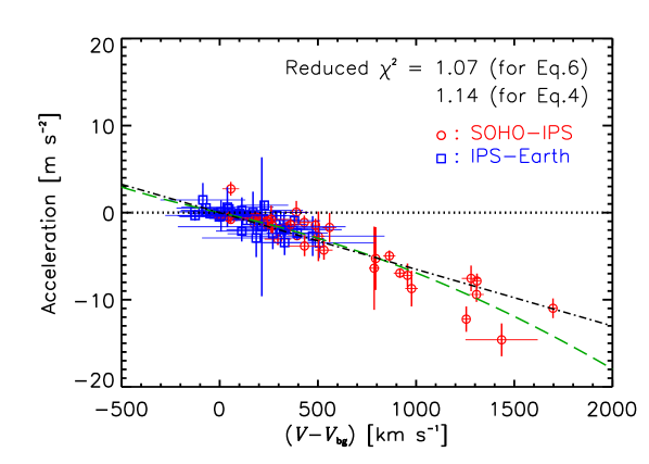
Figure 6.: Relationship between acceleration $a$ and difference in speed ${(V-V_{\mathrm{bg}})}$ for 40 fast and moderate ICMEs identified in this study. Circles (red) and squares (blue) denote data points in the SOHO–IPS and IPS–Earth regions, respectively. The dotted line shows the zero-acceleration line. The dash–dotted (black) line and the dashed (green) line denote the acceleration-speed profiles of Equation (eq.previous) and Equation (eq.modified), respectively. fig6

Equations (eq.linear) and (eq.gamma) are similar to a set of simultaneous equations in the “snow plough” model proposed by Tappin2006. While he explained that ICMEs decelerate by the momentum transfer with piling up mass in front of them, we will explain their acceleration in terms of fluid dynamics. When an object propagates in a fluid, the object suffers the drag force due to the interaction with the surrounding medium. The characteristics of drag force changes depending on the Reynolds number $\mathrm{Re}=({\rho}dU)/{\mu}=(dU)/{\nu}$, where ${\rho}$, $d$, $U$, and ${\mu}$ are fluid density, the size and speed of the object, and viscosity of the fluid, respectively, and ${\nu}$ is the kinematic viscosity defined as ${{\nu}={\mu}/{\rho}}$. The drag force is proportional to $U$ for ${\mathrm{Re}\ll 1}$ and to ${U^{2}}$ for ${\mathrm{Re}\gg 1}$. The former is called the hydrodynamic Stokes drag force, while the latter corresponds to the aerodynamic drag force. Borgazzi et al. (2008, 2009) discussed the ICME propagation using a model involving both drag forces by assuming a spherical body of ICMEs. They assumed that ICMEs undergo both Stokes and aerodynamic drag forces during their propagation.

Here, we note that Equation (eq.modified) consists of quadratic and linear terms, which can be interpreted to be due to the aerodynamic and Stokes drag forces, respectively. In order to understand the character of this equation, we assess the contribution from each term to the net acceleration. Such contributions were calculated by applying various solar-wind speeds to Equation (eq.modified), and are listed in Table table10. We confirm from this table that the contribution from each term varies with the difference in speed, and the linear term (Stokes drag force) has a larger contribution than the quadratic term (aerodynamic drag force) to the net acceleration in a speed range of ${0}$ ${{\mathrm{km~{}s^{-1}}}}$ $\leq V-V_{\mathrm{bg}}\leq 2300$ ${\mathrm{km~{}s^{-1}}}$. This result suggests that ICMEs with the above speed range are controlled mainly by the Stokes drag force, while the aerodynamic drag force is a predominant factor for the propagation of ICMEs with ${V-V_{\mathrm{bg}}>2300}$ ${\mathrm{km~{}s^{-1}}}$. This interpretation is consistent with the fundamental theory of fluid dynamics because ${\mathrm{Re}\propto V}$. However, ICMEs with $V-V_{\mathrm{bg}}>2300$ ${\mathrm{km~{}s^{-1}}}$ are extremely fast eruptions having the propagation speed exceeding 2800 ${\mathrm{km~{}s^{-1}}}$, and so are very rare Gopalswamy et al. (2009). Therefore, we conclude that the Stokes drag force will play the key role for almost all of the fast and moderate ICMEs.

Table 6.: Contributions of linear and quadratic terms to the net acceleration versus the difference in speed (${V-V_{\mathrm{bg}}}$) in Equation (eq.modified). table10

${(V-V_{\mathrm{bg}})}$	Net acceleration	Linear term	Quadratic term
[${\mathrm{km~{}s^{-1}}}$]	[${\mathrm{m~{}s^{-2}}}$]	contrib. [%]	contrib. [%]
100	$-0.51$	95.9	4.1
500	$-2.94$	82.4	17.6
1000	$-6.91$	70.1	29.9
1500	$-11.92$	60.9	39.1
2000	$-17.97$	53.9	46.1
2100	$-19.30$	52.7	47.3
2200	$-20.68$	51.5	48.5
2300	$-22.09$	50.4	49.6
2400	$-23.55$	49.4	50.6
2500	$-25.05$	48.4	51.6
3000	$-33.16$	43.8	56.2

4.3 Kinematic Viscosity and Drag Coefficient for the ICME–Solar Wind Interaction

viscosity

Furthermore, Equation (eq.modified) also implies that the effective kinematic viscosity of the solar wind (${{\nu}_{\mathrm{SW}}}$) exhibits a large value in the ICME–solar wind interaction system. Now, we estimate the value of ${{\nu}_{\mathrm{SW}}}$. Borgazzi2008 pointed out that the drag force is represented by $F=-6{\pi}{\nu}{\rho}d(V-V_{\mathrm{bg}})$ for ${\mathrm{Re}\ll 1}$ by assuming a spherical body of ICMEs. We apply this expression to the linear term in Equation (eq.modified), and find

$$\ilabel{eq.viscosity}\frac{6{\pi}{\nu}_{\mathrm{SW}}{\rho}_{\mathrm{SW}}d}{m}=4.84\times 10^{-6}~{}{\mathrm{s^{-1}}},$$ (7)

where ${{\rho}_{\mathrm{SW}}}$, $d$, and $m$ are the solar wind density, radial size, and mass of ICMEs, respectively. Substituting the values of $d=4.49\times 10^{10}$ m (${=0.3}$ AU) Richardson and Cane (2010), $m=1.7\times 10^{12}$ kg Vourlidas et al. (2002), and ${\rho}_{\mathrm{SW}}=1.67\times 10^{-22}$ ${\mathrm{kg~{}m^{-3}}}$ (in other words, the total mass density of 10 protons per cubic centimeter) in the above equation, we obtain ${{\nu}_{\mathrm{SW}}=5.8\times 10^{16}}$ ${\mathrm{m^{2}~{}s^{-1}}}$. This value is an order of magnitude smaller than the viscosity estimated by Lara2011. On the other hand, if we use the value of viscosity estimated by them, we may estimate the mass of ICMEs instead of ${{\nu}_{\mathrm{SW}}}$. Lara2011 reported ${\nu}_{\mathrm{SW}}=1.55\times 10^{17}$ ${\mathrm{m^{2}~{}s^{-1}}}$ (from the speed matching method) and ${2.60\times 10^{17}}$ ${\mathrm{m^{2}~{}s^{-1}}}$ (from the time matching method) as the value of viscosity. Substituting this value into Equation (eq.viscosity) with the above $d$ and ${\rho}_{\mathrm{SW}}$ values, we obtain $m\approx 10^{13}$ kg. This value corresponds to the upper limit of CME mass observed using SOHO/LASCO Gopalswamy et al. (2009). Therefore, this analysis corroborates our expectation in Paper I that ICMEs detected by the IPS observations are probably massive events.

Borgazzi2008 also showed that the drag force is described by $F=-(\mathrm{C_{d}}A{\rho})/2(V-V_{\mathrm{bg}})^{2}$ for ${\mathrm{Re}\gg 1}$, where $\mathrm{C_{d}}$ and $A$ are the dimensionless drag coefficient and cross section of ICMEs, respectively. By applying this expression to the quadratic term in Equation (eq.modified) with $A={\pi}({d/2})^{2}$, we can estimate the value of $\mathrm{C_{d}}$. Using the following equation:

$$\ilabel{eq.coefficient}\frac{{\mathrm{C_{d}}}{\rho}_{\mathrm{SW}}{\pi}d^{2}}{8m}=2.07\times 10^{-12}~{}{\mathrm{m^{-1}}},$$ (8)

and the above values of $m$, $d$, and ${\rho}_{\mathrm{SW}}$, we find $\mathrm{C_{d}}=27$. This value is almost three orders of magnitude smaller than the estimation by Lara2011; they reported ${\mathrm{C_{d}}=2.63\times 10^{3}}$ (from the speed matching method) and ${1.08\times 10^{4}}$ (from the time matching method). Borgazzi2009 reported that $\mathrm{C_{d}}$ is ${0.6\times 10^{5}}$ – ${1.6\times 10^{5}}$ (considering the variation in radius) or ${2\times 10^{4}}$ – ${8\times 10^{4}}$ (considering the density variation) for the turbulent regime. On the other hand, Cargill2004 showed by numerical simulations that $\mathrm{C_{d}}$ varies slowly between the Sun and the Earth, and is roughly unity for dense ICMEs. He also showed that when the ICME and solar wind densities are similar, $\mathrm{C_{d}}$ is larger than unity (between 3 and 10), but remains approximately constant with the radial distance. As shown here, each researcher reports different values of $\mathrm{C_{d}}$, and so it is difficult to determine its real value.

5 Summary and Conclusions

conclusion

We investigated kinematic properties of six slow (${V_{\mathrm{SOHO}}-V_{\mathrm{bg}}<0}$ ${\mathrm{km~{}s^{-1}}}$), 25 moderate (${0}$ ${\mathrm{km~{}s^{-1}}}$ ${\leq V_{\mathrm{SOHO}}-V_{\mathrm{bg}}\leq 500}$ ${\mathrm{km~{}s^{-1}}}$), and 15 fast ($V_{\mathrm{SOHO}}-V_{\mathrm{bg}}>500$ ${\mathrm{km~{}s^{-1}}}$) ICMEs detected by SOHO/LASCO, IPS, and in-situ observations during 1997 – 2011.

Our analyses for the slow ICMEs show the following results: i) They accelerate toward the speed of the background solar wind during their propagation, and attain their final speed by ${0.34\pm 0.03}$ AU. ii) The acceleration ends when they reach ${479\pm 126}$ ${\mathrm{km~{}s^{-1}}}$; this is close to the typical speed of the solar wind during the period of this study. Examinations of the relationship between the difference in speed and the acceleration and the assessment of significance level for them show that iii) Equation (eq.quadratic) with ${\gamma}_{\mathrm{2}}=2.36~{}(\pm 1.03)\times 10^{-11}$ $\mathrm{m^{-1}}$ is more suitable than Equation (eq.linear) to describe the kinematics of slow ICMEs. The result iii) is consistent with earlier studies by Maloney2010 and Byrne2010. However, six events of slow ICMEs in our sample are not sufficient to investigate their kinematics more precisely. Therefore, we need to identify more slow ICMEs and then examine their kinematics carefully.

We also found from examinations of fast and moderate ICMEs that the value of coefficient ${{\gamma}_{\mathrm{1}}}$ has speed dependence described by Equation (eq.gamma). On the basis of these, we find a modified equation, $a=-2.07\times 10^{-12}$$(V-V_{\mathrm{bg}})|V-V_{\mathrm{bg}}|$ $-4.84\times 10^{-6}(V-V_{\mathrm{bg}})$, for the ICME motion. We interpret this equation as indicating that ICMEs with ${0}$ ${\mathrm{km~{}s^{-1}}}$ $\leq V-V_{\mathrm{bg}}\leq 2300$ ${\mathrm{km~{}s^{-1}}}$ are controlled mainly by the Stokes drag force, while the aerodynamic drag force is a predominant factor for the propagation of ICMEs with $V-V_{\mathrm{bg}}>2300$ ${\mathrm{km~{}s^{-1}}}$. Because such extremely fast ICMEs are very rare, we conclude that the Stokes drag force will play the key role for almost all of the fast and moderate ICMEs.

We also estimated the effective kinematic viscosity of the solar wind (${{\nu}_{\mathrm{SW}}}$) and the dimensionless drag coefficient ($\mathrm{C_{d}}$) in the ICME–solar wind interaction system. Combining the linear term in the modified equation and $F=-6{\pi}{\nu}{\rho}d(V-V_{\mathrm{bg}})$, we obtain ${\nu}_{\mathrm{SW}}=5.8\times 10^{16}$ ${\mathrm{m^{2}~{}s^{-1}}}$; this is an order of magnitude smaller than the value in an earlier study by Lara2011. By comparing the quadratic term in the modified equation with $F=-(\mathrm{C_{d}}A{\rho})/2(V-V_{\mathrm{bg}})^{2}$, we find $\mathrm{C_{d}}=27$ for the value of drag coefficient.

Acknowledgements

The IPS observations were carried out under the solar wind program of the Solar-Terrestrial Environment Laboratory (STEL) of Nagoya University. We acknowledge use of the SOHO/LASCO CME catalog; this CME catalog is generated and maintained at the CDAW Data Center by the National Aeronautics and Space Administration (NASA) and the Catholic University of America in cooperation with the Naval Research Laboratory. SOHO is a project of international cooperation between the European Space Agency and NASA. We thank the Space Physics Data Facility of NASA’s Goddard Space Flight Center for use of OMNIWeb service and OMNI data.

References

- Asai et al. (1995) Asai, K., Ishida, Y., Kojima, M., Maruyama, K., Misawa, H., Yoshimi, N.: 1995, Multi-station system for solar wind observations using the interplanetary scintillation method. J. Geomagn. Geoelectr. 47, 1107 – 1112.
- Borgazzi et al. (2008) Borgazzi, A., Lara, A., Romero-Salazar, L., Ventura, A.: 2008, Transport in the interplanetary medium of coronal mass ejections. Geofis. Int. 47, 301 – 310.
- Borgazzi et al. (2009) Borgazzi, A., Lara, A., Echer, E., Alves, M.V.: 2009, Dynamics of coronal mass ejections in the interplanetary medium. A&A 498, 885 – 889.
- Brueckner et al. (1995) Brueckner, G.E., Howard, R.A., Koomen, M.J., Korendyke, C.M., Michels, D.J., Moses, J.D., et al.: 1995, The Large Angle Spectroscopic Coronagraph (LASCO). Sol. Phys. 162, 357 – 402.
- Brueckner et al. (1998) Brueckner, G.E., Delaboudiniere, J.P., Howard, R.A., Paswaters, S.E., St. Cyr, O.C., Schwenn, R., Lamy, P., Simnett, G., Thompson, B., Wang, D.: 1998, Geomagnetic storms caused by coronal mass ejections (CMEs): March 1996 through June 1997. Geophys. Res. Lett. 25, 3019 – 3022.
- Byrne et al. (2010) Byrne, J.P., Maloney, S.A., McAteer, R.J., Refojo, J.M., Gallagher, P.T.: 2010, Propagation of an earth-directed coronal mass ejection in three dimensions. Nature Comm. 1, 74.
- Cane, Richardson, and St. Cyr, O.C. (2000) Cane, H., Richardson, I., St. Cyr, O.C.: 2000, Coronal mass ejections, interplanetary ejecta and geomagnetic storms. Geophys. Res. Lett. 27, 3591 – 3594.
- Cargill (2004) Cargill, P.J.: 2004, On the aerodynamic drag force acting on interplanetary coronal mass ejections. Sol. Phys. 221, 135 – 149.
- Chen (1996) Chen, J.: 1996, Theory of prominence eruption and propagation: Interplanetary consequences. J. Geophys. Res. 101, 27499 – 27520.
- Gapper et al. (1982) Gapper, G.R., Hewish, A., Purvis, A., Duffett-Smith, P.J.: 1982, Observing interplanetary disturbances from the ground. Nature 296, 633 – 636.
- Gloeckler et al. (1998) Gloeckler, G., Cain, J., Ipavich, F.M., Tums, E.O., Bedini, P., Fisk, L.A., et al.: 1998, Investigation of the composition of solar and interstellar matter using solar wind and pickup ion measurements with SWICS and SWIMS on the ACE spacecraft. Space Sci. Rev. 86, 497 – 539.
- Gopalswamy et al. (2000) Gopalswamy, N., Lara, A., Lepping, R.P., Kaiser, M.L., Berdichevsky, D., St. Cyr, O.C.: 2000, Interplanetary acceleration of coronal mass ejections. Geophys. Res. Lett. 27, 145 – 148.
- Gopalswamy et al. (2001) Gopalswamy, N., Lara, A., Yashiro, S., Kaiser, M.L., Howard, R.A.: 2001, Predicting the 1-AU arrival times of coronal mass ejections. J. Geophys. Res. 106, 29207 – 29218.
- Gopalswamy et al. (2009) Gopalswamy, N., Yashiro, S., Michalek, G., Stenborg, G., Vourlidas, A., Freeland, S., Howard, R.: 2009, The SOHO/LASCO CME Catalog. Earth Moon Planets 104, 295 – 313.
- Gosling et al. (1991) Gosling, J., McComas, D., Phillips, J., Bame, S.: 1991, Geomagnetic activity associated with earth passage of interplanetary shock disturbances and coronal mass ejections. J. Geophys. Res. 96, 7831 – 7839.
- Guhathakurta and Fisher (1998) Guhathakurta, M., Fisher, R.: 1998, Solar wind consequences of a coronal hole density profile: Spartan 201-03 coronagraph and Ulysses observations from 1.15 to 4 AU. ApJ 499, L215 – L218.
- Hewish, Scott, and Wills (1964) Hewish, A., Scott, P.F., Wills, D.: 1964, Interplanetary scintillation of small diameter radio sources. Nature 203, 1214 – 1217.
- Howard (2011) Howard, T.: 2011, Coronal Mass Ejections: An Introduction, Springer, New York, 4.
- Iju, Tokumaru, and Fujiki (2013) Iju, T., Tokumaru, M., Fujiki, K.: 2013, Radial speed evolution of coronal mass ejections during solar cycle 23. Sol. Phys. 288, 331 – 353. (Paper I).
- Kojima and Kakinuma (1990) Kojima, M., Kakinuma, T.: 1990, Solar cycle dependence of global distribution of solar wind speed. Space Sci. Rev. 53, 173 – 222.
- Lara et al. (2011) Lara, A., Flandes, A., Borgazzi, A., Subramanian, P., México, C.U.: 2011, Velocity profile of interplanetary coronal mass ejections beyond 1 AU. J. Geophys. Res. 116, A12102.
- Lindsay et al. (1999) Lindsay, G.M., Luhmann, J.G., Russell, C.T., Gosling, J.T.: 1999, Relationships between coronal mass ejection speeds from coronagraph images and interplanetary characteristics of associated interplanetary coronal mass ejections. J. Geophys. Res. 104, 12515 – 12524.
- Lynch et al. (2010) Lynch, B.J., Li, Y., Thernisien, A.F.R., Robbrecht, E., Fisher, G.H., Luhmann, J.G., Vourlidas, A.: 2010, Sun to 1 AU propagation and evolution of a slow streamer-blowout coronal mass ejection. J. Geophys. Res. 115, A07106.
- Maloney and Gallagher (2010) Maloney, S.A., Gallagher, P.T.: 2010, Solar wind drag and the kinematics of interplanetary coronal mass ejections. ApJ 724, L127 – L132.
- Manoharan (2006) Manoharan, P.K.: 2006, Evolution of coronal mass ejections in the inner heliosphere: A study using white-light and scintillation images. Sol. Phys. 235, 345 – 368.
- Reiner, Kaiser, and Bougeret (2003) Reiner, M.J., Kaiser, M.L., Bougeret, J.L.: 2003, On the deceleration of CMEs in the corona and interplanetary medium deduced from radio and white-light observations. In: Velli, M., Bruno, R., Malara, F. (eds.) Solar Wind Ten: Proceedings of the Tenth International Solar Wind Conference, AIP Conf. Proc. 679, 152 – 155.
- Richardson and Cane (2010) Richardson, I.G., Cane, H.V.: 2010, Near-earth interplanetary coronal mass ejections during solar cycle 23 (1996–2009): Catalog and summary of properties. Sol. Phys. 264, 189 – 237.
- Rollett et al. (2012) Rollett, T., Möstl, C., Temmer, M., Veronig, A.M., Farrugia, C.J., Biernat, H.K.: 2012, Constraining the kinematics of coronal mass ejections in the inner heliosphere with in-situ signatures. Sol. Phys. 276, 1 – 22.
- Schwenn et al. (1981) Schwenn, R., Mühlhäuser, K.H., Marsch, E., Rosenbauer, H.: 1981, Two states of the solar wind at the time of solar activity minimum, II Radial gradient of plasma parameters in fast and slow streams. In: Rosenbauer, H. (ed.) Solar Wind Four, Max-Plank-Institute für Aeronomie, Katlenburg-Lindau, 126 – 130.
- Shanmugaraju et al. (2009) Shanmugaraju, A., Moon, Y.-J., Vrsnak, B., Vrbanec, D.: 2009, Radial evolution of well-observed slow cmes in the distance range 2–30 . Sol. Phys. 257, 351 – 361.
- Sheeley et al. (1997) Sheeley, N.R. Jr., Wang, Y.-M., Hawley, S.H., Brueckner, G.E., Dere, K.P., Howard, R.A., et al.: 1997, Measurements of flow speeds in the corona between 2 and 30 . ApJ 484, 472 – 478.
- Shen et al. (2011) Shen, C., Wang, Y., Gui, B., Ye, P., Wang, S.: 2011, Kinematic evolution of a slow cme in corona viewed by STEREO-B on 8 October 2007. Sol. Phys. 269, 389 – 400.
- Stone et al. (1998) Stone, E.C., Frandsen, A.M., Mewaldt, R.A., Christian, E.R., Margolies, D., Ormes, J.F., Snow, F.: 1998, The Advanced Composition Explorer. Space Sci. Rev. 86, 1 – 22.
- Tappin (2006) Tappin, S.J.: 2006, The deceleration of an interplanetary transient from the sun to 5 AU. Sol. Phys. 233, 233 – 248.
- Temmer et al. (2011) Temmer, M., Rollett, T., Möstl, C., Veronig, A.M., Vršnak, B., Odstrčil, D.: 2011, Influence of the ambient solar wind flow on the propagation behavior of interplanetary coronal mass ejections. ApJ 743, 101 – 112.
- Tokumaru et al. (2011) Tokumaru, M., Kojima, M., Fujiki, K., Maruyama, K., Maruyama, Y., Ito, H., Iju, T.: 2011, A newly developed UHF radiotelescope for interplanetary scintillation observations: Solar wind imaging facility. Radio Sci. 46, RS0F02.
- Vourlidas et al. (2002) Vourlidas, A., Buzasi, D., Howard, R.A., Esfandiari, E.: 2002, Mass and energy properties of LASCO CMEs. In: Wilson, A. (ed.) Solar Variability: From Core to Outer Frontiers,ESA SP-506, 91 – 94.
- Vršnak and Gopalswamy (2002) Vršnak, B., Gopalswamy, N.: 2002, Influence of the aerodynamic drag on the motion of interplanetary ejecta. J. Geophys. Res. 107, 1019.
- Vršnak et al. (2010) Vršnak, B., Žic, T., Falkenberg, T.V., Möstl, C., Vennerstrom, S., Vrbanec, D.: 2010, The role of aerodynamic drag in propagation of interplanetary coronal mass ejections. A&A 512, A43.
- Vršnak et al. (2013) Vršnak, B., Žic, T., Vrbanec, D., Temmer, M., Rollett, T., Möstl, C., et al.: 2013, Propagation of interplanetary coronal mass ejections: The drag-based model. Sol. Phys. 285, 295 – 315.
- Yashiro et al. (2004) Yashiro, S., Gopalswamy, N., Michalek, G., St. Cyr, O.C., Plunkett, S.P., Rich, N.B., Howard, R.A.: 2004, A catalog of white light coronal mass ejections observed by the SOHO spacecraft. J. Geophys. Res. 109, A07105.