Glassy Chimeras Could Be Blind to Quantum Speedup:
Designing
Better Benchmarks for Quantum Annealing Machines
Abstract
Recently, a programmable quantum annealing machine has been built that minimizes the cost function of hard optimization problems by, in principle, adiabatically quenching quantum fluctuations. Tests performed by different research teams have shown that, indeed, the machine seems to exploit quantum effects. However experiments on a class of random-bond instances have not yet demonstrated an advantage over classical optimization algorithms on traditional computer hardware. Here we present evidence as to why this might be the case. These engineered quantum annealing machines effectively operate coupled to a decohering thermal bath. Therefore, we study the finite-temperature critical behavior of the standard benchmark problem used to assess the computational capabilities of these complex machines. We simulate both random-bond Ising models and spin glasses with bimodal and Gaussian disorder on the D-Wave Chimera topology. Our results show that while the worst-case complexity of finding a ground state of an Ising spin glass on the Chimera graph is not polynomial, the finite-temperature phase space is likely rather simple because spin glasses on Chimera have only a zero-temperature transition. This means that benchmarking optimization methods using spin glasses on the Chimera graph might not be the best benchmark problems to test quantum speedup. We propose alternative benchmarks by embedding potentially harder problems on the Chimera topology. Finally, we also study the (reentrant) disorder-temperature phase diagram of the random-bond Ising model on the Chimera graph and show that a finite-temperature ferromagnetic phase is stable up to 19.85(15)% antiferromagnetic bonds. Beyond this threshold, the system only displays a zero-temperature spin-glass phase. Our results therefore show that a careful design of the hardware architecture and benchmark problems is key when building quantum annealing machines.
pacs:
75.50.Lk, 75.40.Mg, 05.50.+q, 03.67.LxI Introduction
Quantum devices are gaining an increasing importance in everyday technology: They find applications in different technological areas such as (true) quantum random number generators, as well as quantum encryption systems for data transmission. The holy grail is to build a programmable quantum simulator with capabilities exceeding “traditional” computer hardware based on classical bits. The first programmable commercial device that attempts to exploit the unique power of quantum mechanics to perform computations is the D-Wave One quantum annealer com (a). In analogy to simulated annealing Kirkpatrick et al. (1983) where thermal fluctuations are adiabatically quenched to minimize a cost function, this machine is based on the quantum annealing optimization method Finnila et al. (1994); Kadowaki and Nishimori (1998); Kadowaki (1998); Brooke et al. (1999); Martoňák et al. (2002); Santoro et al. (2002); Santoro and Tosatti (2006); Das and Chakrabarti (2005, 2008) where quantum fluctuations replace thermal ones.
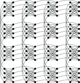
Tests by different research teams suggest that, indeed, the D-Wave quantum annealer likely optimizes using quantum effects Johnson et al. (2011); Boixo et al. (2013, 2013); Wang et al. (2013); Dickson et al. (2013). Although it has been shown theoretically Morita and Nishimori (2008), as well as with numerical experiments Santoro et al. (2002); com (b) that quantum annealing could, in principle, outperform classical (thermal) optimization algorithms (such as simulated annealing Kirkpatrick et al. (1983)) on an algorithmic level, when applied to a class of random edge-weight instances, the quantum annealing machine has not yet shown a speedup over classical optimization methods Boixo et al. (2013); Rønnow et al. (2014). In this work, we present evidence for why this might be the case: The D-Wave One and Two quantum annealing machines use a restrictive “Chimera” topology (see Fig. 1 for an example with 128 quantum bits) imposed because of fabrication constraints of the solid-state quantum bits.
Probably the best benchmark problem to test the efficiency of optimization algorithms is a spin glass Binder and Young (1986); Lucas (2014). Both the disorder and frustration produce a complex energy landscape that challenges optimization algorithms. As such, all current benchmarks of the quantum annealing machine attempt to find the ground state of a certain class of Ising spin glass on the Chimera topology. However, as shown in this work, instances belonging to this class of Ising spin glasses on the Chimera topology only have a spin-glass phase at zero temperature. Furthermore, the energy landscape of such problems seems to be simpler down to low temperatures than for a system with a finite-temperature transition because correlations only build up very close to absolute zero. Because quantum annealing excels in tunneling through barriers—barriers that do not seem to be very pronounced at finite, but low temperatures in this case—classical annealing schedules might typically have an advantage for this particular class of systems.
Although the worst-case complexity of finding a ground state of an Ising spin glass on the Chimera topology is worse than polynomial Barahona (1982), it seems that the fact that the system only orders at zero temperature allows for an easier determination of typical ground-state instances using heuristic classical approaches Boixo et al. (2013); com (c). As such, Ising spin glasses on the Chimera topology live up to their name: an amalgamation of both ordinary and complex behavior.
We reach this conclusion by studying the critical behavior of Ising spin glasses with both Gaussian and bimodal random bonds on the Chimera topology, as well as the random-bond Ising model. Based on our findings, we propose stronger benchmark problems by embedding on the Chimera topology problems that should have a finite-temperature transition and thus might be harder to optimize. Furthermore, our results show that a careful design of the hardware architecture and benchmark problems is key when building quantum annealing machines.
We should also mention that while the results of this paper provide a plausible explanation for the scaling behavior observed so far on random-bond Ising problems, it is also known that on quantum annealer implementations, the couplers and biases are influenced by various sources of noise and error, as demonstrated by the fact that gauge-transformed specifications of the same problem can give substantially different performance Boixo et al. (2013). Classical simulated annealing does not, of course, have this issue, and it is currently unclear how much loss of efficiency these errors cause for the hardware.
II Model, Observables, and Algorithm
We study the spin-glass Hamiltonian
| (1) |
with Ising spins on the nodes of the Chimera graph. An example of the topology with blocks of spins is shown in Fig. 1. A chimera graph with blocks has spins and a characteristic linear length scale of . The interactions are either chosen from a Gaussian disorder distribution with zero mean and unit variance or from a bimodal distribution , where with a probability a bond is ferromagnetic.
Ordering in spin glasses is detected from the spin overlap , where “” and “” are two independent spin replicas with the same disorder. In the ferromagnetic case, order is measured via the magnetization, i.e., . To detect the existence of a phase transition to high precision, we measure the Binder ratio Binder (1981) , where represents either the magnetization for the ferromagnetic sector or the spin overlap in the spin-glass sector. The Binder ratio is a dimensionless function, which means that, at a putative transition, data for different characteristic system sizes will cross when , where is the critical temperature (up to corrections to scaling). This means . Using a finite-size scaling analysis, the critical temperature and the critical exponent can be determined. To uniquely determine the universality class of a system, two critical exponents are needed Yeomans (1992). To this end, we also measure the susceptibility , where again represents either the magnetization for the ferromagnetic sector, or the spin-glass order parameter for the spin-glass sector. The susceptibility scales as , where is an independent critical exponent.
Simulations are done using the replica exchange Monte Carlo Hukushima and Nemoto (1996) method, and simulation parameters are listed in Table 1. Note that for each disorder instance we simulate two independent replicas to compute the spin-glass overlap. In the Gaussian case, we test equilibration using the method developed in Ref. Katzgraber et al. (2001) adapted to the Chimera topology. For bimodal disorder, we perform a logarithmic binning of the data. Once the last four bins agree within error bars, we deem the system to be in thermal equilibrium. To obtain optimal values for the critical parameters, we determine these via the analysis method pioneered in Ref. Katzgraber et al. (2006), where the critical parameters are optimized using a Levenberg-Marquard minimization until the chi square of a fit to a third-order polynomial is minimal. This approach is then bootstrapped to obtain statistically sound error bars.
| , , | ||||||
|---|---|---|---|---|---|---|
| , , | ||||||
| , , | ||||||
| , , | ||||||
| , , | ||||||
| , , | ||||||
| , , | ||||||
| , , | ||||||
| , , | ||||||
| , , | ||||||
| , , | ||||||
| , , | ||||||
| , | ||||||
| , | ||||||
| , | ||||||
| , | ||||||
| , | ||||||
| , | ||||||
| , | ||||||
| , | ||||||
| , | ||||||
| , | ||||||
| , | ||||||
| , | ||||||
| Gauss | ||||||
| Gauss | ||||||
| Gauss | ||||||
| Gauss |
III Results within the spin-glass sector
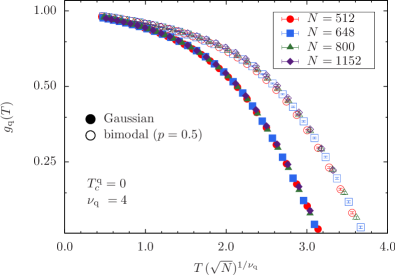
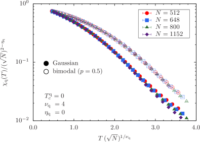
Figure 2 shows a finite-size scaling analysis of the Binder ratio (top panel) for both Gaussian disorder (full symbols) and bimodal disorder with (open symbols) in a semilogarithmic scale. The data scale extremely well, even far from the spin-glass transition temperature. We find that for both cases, we have the same critical parameters, namely com (d)
| (2) |
Note that spin glasses on two-dimensional square lattices have Katzgraber et al. (2004); i.e., spin glasses on the Chimera topology are close to two space dimensions.
Interestingly, the phase transition to a spin-glass phase only occurs at zero temperature, despite the Chimera graph being nonplanar. Furthermore, the divergence of the correlation length is rather violent, with for . This suggests that the phase space and correlations only build up close to for a spin glass defined on the Chimera topology. One of the potential advantages of a quantum algorithm over a classical one lies in its ability to tunnel through barriers. Classical algorithms must “climb” over these barriers com (e). The aforementioned results imply that the barriers of a spin glass defined on a Chimera graph at nonzero temperature seem to be of “finite” height, while for any Ising spin glass with a finite transition temperature the barriers diverge below for decreasing temperature and increasing system size . This could offer one explanation for why quantum annealing machines, such as D-Wave One and Two, cannot find a noticeable speedup over classical algorithms such as vanilla simulated annealing Kirkpatrick et al. (1983) on this class of problems. Furthermore, a spin glass on a Chimera graph seems to order in an almost “discontinuous” fashion at zero temperature with the highly-connected blocks of eight spins behaving like a “super spin” on a two-dimensional–like planar lattice. Once the individual blocks order, the whole system suddenly orders. It is well known that quantum annealing has problems when first-order transitions are present Young et al. (2008); Amin and Choi (2009); Young et al. (2010); Hen and Young (2011); i.e., this could be the second reason why quantum annealing machines do not seem to outperform simple classical optimization methods on these problems.
IV Results within the ferromagnetic sector
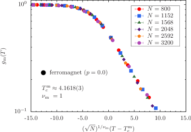
For completeness, we also study the Ising ferromagnet on the Chimera graph and compute the disorder (fraction of ferromagnetic bonds) vs temperature phase diagram of the model. For no disorder, i.e., the pure ferromagnet where , in Eq. (1), an Ising model on the Chimera graph displays a two-dimensional-Ising-model-like behavior. Figure 3, top panel, shows a finite-size scaling analysis of the ferromagnetic Binder ratio as a function of the scaling variable . The data scale extremely well for and . Note that the obtained value for the critical exponent agrees with the value for the two-dimensional Ising ferromagnet Yeomans (1992), therefore corroborating our assumption that the system might behave similarly to a two-dimensional superspin Ising model.
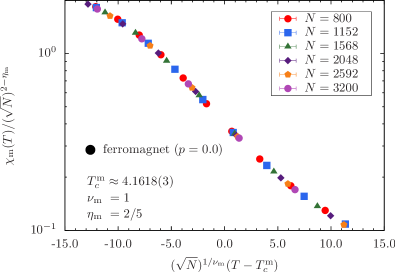
Figure 3, bottom panel, shows a finite-size scaling analysis of the ferromagnetic susceptibility as a function of using the estimate of the critical temperature determined from the finite-size scaling of the Binder ratio. The data scale very well with very small corrections to scaling using and . Note that the value of the critical exponent is slightly larger, yet close to the exact value of the two-dimensional Ising model (). Therefore, an Ising ferromagnet on the Chimera graph and the two-dimensional Ising model do not share the same universality class com (f). In summary,
| (3) |
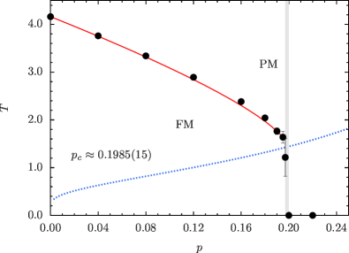
Finally, we study the random-bond version of the Ising model on the Chimera graph where a fraction of ferromagnetic bonds is antiferromagnetic. We vary and compute the critical temperature of the ferromagnetic phase. Figure 4 shows the (critical) temperature vs disorder phase diagram. The dotted (blue) line represents the Nishimori condition Nishimori (1981) . At the point where the phase boundary (solid line) crosses the Nishimori line, i.e., for , ferromagnetic order is lost. This means that for any finite temperature and , a random-bond Ising model on the Chimera graph is essentially a disordered ferromagnet and is easily solved with a conventional optimization algorithm. Therefore, to compare a quantum adiabatic optimizer to any classical optimization method, strong enough disorder is needed.
V Discussion
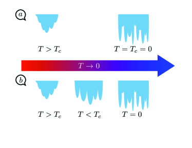
Figure 5 shows cartoons of the energy landscape for a system with a zero-temperature transition [panel (a), top] and a finite-temperature transition [panel (b), bottom] to a spin-glass state. When the temperature is above the putative critical temperature , the energy landscape is typically simple with one dominant minimum. For a system that has a finite-temperature transition and for temperatures , the energy landscape becomes rough with barriers that grow with decreasing temperature and increasing system size until the ground state of the system is reached. However, for a system where , such as spin glasses on the Chimera topology, the energy landscape is likely much simpler until close to the ground state. This means that for such a system, a classical annealing schedule should perform well in comparison to quantum annealing which, in theory, excels when the energy landscape has diverging barriers. Note also that when the system with bimodal disorder is in the ferromagnetic phase (), the energy landscape is also simpler and reminiscent of the cartoon shown in the left-most panels of Fig. 5. This means that benchmarking quantum annealing machines that operate at low, but finite temperatures using spin glasses on a Chimera topology is likely not the best approach. Indeed, recent studies in a field Dash (2013); Saket (2013) have shown that spin-glass instances can be efficiently computed classically, albeit still scaling exponentially. However, because there is likely no spin-glass state in a field Young and Katzgraber (2004); Jörg et al. (2008); Katzgraber et al. (2009a); Baity-Jesi et al. (2013), this is no surprise. To truly discern if quantum annealing machines (defined on the Chimera topology) display an advantage over classical annealing algorithms, problems that display a finite-temperature transition and have a rough energy landscape for a range of finite temperatures need to be embedded in the machine’s topology. Given the current hardware constraints, we propose the following benchmarks:
Three-dimensional cubic lattices.— The system has a finite-temperature transition to a spin-glass state at for Gaussian disorder ( for bimodal disorder and ) Katzgraber et al. (2006). We estimate that a Chimera graph of qubits could be used to embed a relatively modest 3D system of spins with periodic boundary conditions and one of size with free boundary conditions. Note that current state-of-the art classical optimization algorithms Hartmann and Rieger (2001, 2004) can estimate ground states to high accuracy of up to approximately spins.
Viana-Bray model.— The Ising spin glass is defined on a random graph with average connectivity Viana and Bray (1985); Katzgraber et al. (2001). For any , the system has a finite-temperature phase transition into a spin-glass state. To simplify the embedding, a random graph with Gaussian disorder and could be studied, where . However, to be able to embed the long-range connections between the spins, we estimate that qubits might be needed to embed a system with spins like in the mean-field Sherrington-Kirkpatrick model Sherrington and Kirkpatrick (1975); Choi (2008, 2011).
Rescaled Chimera systems.— It is plausible that if the ratio of interactions within the cells and between the cells changes proportional to the system size, a mean-field-like finite-temperature spin-glass transition might emerge. For example, the random intercell interactions could be rescaled with [where is a nondecreasing function of the system size] while leaving the random intracell interactions untouched. We attempted to weaken the effects of the tightly bound intercell spin clusters in the Chimera graph by setting the spin-spin interactions to of all intracell interactions (on average). Although universality considerations would suggest that should still be zero when , our data for systems up to approximately spins suggest . We do emphasize, however, that corrections to scaling are huge and a study with far larger systems might be needed.
One could, in principle, also embed a two-dimensional Ising spin glass on a square lattice, where it was first shown by Santoro et al. that quantum annealing might display an advantage over classical annealing via simulations at very low temperatures Santoro et al. (2002). However, ground states of two-dimensional Ising spin glasses can be computed in polynomial time, and the low-temperature behavior of this system is known to be unusual and still controversial Thomas et al. (2011). As such, this might not be a robust and well-controlled benchmark, especially because the D-Wave machines operate at temperatures considerably higher than in the aforementioned study by Santoro et al. Santoro et al. (2002).
The previous examples also illustrate a limitation of the Chimera topology: To embed many systems, a large overhead of quantum bits in the machine to simulated physical bits is needed. This is particularly the case because no long-range connections between the spins are present—a feature that should be included in future chip designs. Finally, at this point it is unclear if the critical behavior of an embedded system is the same as the critical behavior of the actual classical system. This is of utmost importance if one wants to use programmable quantum annealing machines as quantum simulators.
VI Conclusions
Although Barahona Barahona (1982) has rigorously shown that spin glasses defined on graphs like the Chimera topology are worst-case NP-hard types, the Chimera spin glass of the type used so far to compare quantum to classical annealers represents a hard, but typically easier optimization problem. Because such a spin glass on the Chimera topology only orders at zero temperature, classical thermal annealers will typically be able to efficiently estimate ground states for the system. The performance of these classical algorithms would considerably deteriorate if the problem to be optimized exhibits a finite-temperature transition below which energy barriers diverge with decreasing temperature and increasing system size. To be able to show that quantum annealing machines based on the Chimera topology outperform classical annealing schedules, nontrivial embeddings in higher space dimensions or with long-range interactions, as outlined above, are needed. Furthermore, at this point it is unclear how the overhead of the embedding scales with the size of the system and if the embedded system via edge contraction shares the same universality class as the true problem to be emulated—especially when simulated on the actual D-Wave hardware com (i). The latter open questions are the subject of current research and we conclude by emphasizing that the design of the hardware topology in quantum annealing machines is of crucial importance.
Acknowledgements.
We would like to thank F. Barahona, P. Bunyk, J. Machta, R. B. McDonald, C. Moore, M. A. Moore, H. Nishimori, T. F. Rønnow, C. K. Thomas, M. Troyer, A. P. Young, and I. Zintchenko for fruitful discussions. In particular, we would like to thank R. B. McDonald for porting the Python Chimera graph generator to C. H.G.K. acknowledges support from the NSF (Grant No. DMR-1151387) and would also like to thank Bruichladdich Dist. for providing the initial inspiration for this project, as well as the Royal Street Courtyard Inn in New Orleans for their hospitality during the final stages of this manuscript. Finally, we would like to thank the Texas Advanced Computing Center (TACC) at The University of Texas at Austin for providing HPC resources (Lonestar and Stampede Clusters) and Texas A&M University for access to their Eos cluster.References
- com (a) See http://www.dwavesys.com.
- Kirkpatrick et al. (1983) S. Kirkpatrick, C. D. Gelatt, Jr., and M. P. Vecchi, Optimization by simulated annealing, Science 220, 671 (1983).
- Finnila et al. (1994) A. B. Finnila, M. A. Gomez, C. Sebenik, C. Stenson, and J. D. Doll, Quantum annealing: A new method for minimizing multidimensional functions, Chem. Phys. Lett. 219, 343 (1994).
- Kadowaki and Nishimori (1998) T. Kadowaki and H. Nishimori, Quantum annealing in the transverse Ising model, Phys. Rev. E 58, 5355 (1998).
- Kadowaki (1998) T. Kadowaki, Ph.D. thesis, Tokyo Institute of Technology (1998), (quant-ph/0205020).
- Brooke et al. (1999) J. Brooke, D. Bitko, T. F. Rosenbaum, and G. Aepli, Quantum annealing of a disordered magnet, Science 284, 779 (1999).
- Martoňák et al. (2002) R. Martoňák, G. E. Santoro, and E. Tosatti, Quantum annealing by the path-integral Monte Carlo method: The two-dimensional random Ising model, Phys. Rev. B 66, 094203 (2002).
- Santoro et al. (2002) G. Santoro, E. Martoňák, R. Tosatti, and R. Car, Theory of quantum annealing of an Ising spin glass, Science 295, 2427 (2002).
- Santoro and Tosatti (2006) G. E. Santoro and E. Tosatti, TOPICAL REVIEW: Optimization using quantum mechanics: quantum annealing through adiabatic evolution, J. Phys. A 39, R393 (2006).
- Das and Chakrabarti (2005) A. Das and B. K. Chakrabarti, Quantum Annealing and Related Optimization Methods (Edited by A. Das and B.K. Chakrabarti, Lecture Notes in Physics 679, Berlin: Springer, 2005).
- Das and Chakrabarti (2008) A. Das and B. K. Chakrabarti, Quantum Annealing and Analog Quantum Computation, Rev. Mod. Phys. 80, 1061 (2008).
- Johnson et al. (2011) M. W. Johnson, M. H. S. Amin, S. Gildert, T. Lanting, F. Hamze, N. Dickson, R. Harris, A. J. Berkley, J. Johansson, P. Bunyk, et al., Nature 473, 194 (2011).
- Boixo et al. (2013) S. Boixo, T. F. Rønnow, S. V. Isakov, Z. Wang, D. Wecker, D. A. Lidar, J. M. Martinis, and M. Troyer, Quantum annealing with more than one hundred qubits (2013), (arXiv:cond-mat/1304.4595), eprint 1304.4595.
- Boixo et al. (2013) S. Boixo, T. Albash, F. M. Spedalieri, N. Chancellor, and D. A. Lidar, Experimental signature of programmable quantum annealing, Nat. Comm. 4, 2067 (2013).
- Wang et al. (2013) L. Wang, T. F. Rønnow, S. Boixo, S. V. Isakov, Z. Wang, D. Wecker, D. A. Lidar, J. M. Martinis, and M. Troyer, Comment on: ”Classical signature of quantum annealing” (2013), (arxiv:quant-phys/1305.5837).
- Dickson et al. (2013) N. G. Dickson, M. W. Johnson, M. H. Amin, R. Harris, F. Altomare, A. J. Berkley, P. Bunyk, J. Cai, E. M. Chapple, P. Chavez, et al., Thermally assisted quantum annealing of a 16-qubit problem, Nat. Comm. 4, 1903 (2013).
- Morita and Nishimori (2008) S. Morita and H. Nishimori, Mathematical Foundation of Quantum Annealing, J. Math. Phys. 49, 125210 (2008).
- com (b) Detailed tests of the distributions of time scales show that the speedup claimed in Ref. Santoro et al. (2002) could be explained by the fact that the analysis focused only on average times scales and not the distribution of time scales. (M. Troyer, private communication).
- Rønnow et al. (2014) T. F. Rønnow, Z. Wang, J. Job, S. Boixo, S. V. Isakov, D. Wecker, J. M. Martinis, D. A. Lidar, and M. Troyer, Defining and detecting quantum speedup (2014), (arXiv:quant-phys/1401.2910).
- Binder and Young (1986) K. Binder and A. P. Young, Spin glasses: Experimental facts, theoretical concepts and open questions, Rev. Mod. Phys. 58, 801 (1986).
- Lucas (2014) A. Lucas, Ising formulations of many NP problems, Front. Physics 12, 5 (2014).
- Barahona (1982) F. Barahona, On the computational complexity of Ising spin glass models, J. Phys. A 15, 3241 (1982).
- com (c) It is very important to study the distributions of times and not just averages. While the worst-case scenario is that there is at least one instance that cannot be treated efficiently, our claim is that, given the energy landscape, one can expect that the distribution of time scales to probe different ground-state instances likely does not have as fat a tail as, for example, a three-dimensional system with a finite transition temperature. In other words, the number of hard instances is small. However, the vast majority of instances can be treated rather efficiently with simple optimization methods, such as simulated annealing. Finally, all classical optimizers, as well as the D-Wave machine operate at nonzero temperatures. Because the system orders only at zero temperature, the path to low-lying states will be typically easier to reach than if the system had a finite transition temperature where barriers would grow in a more pronounced fashion.
- Binder (1981) K. Binder, Critical properties from Monte Carlo coarse graining and renormalization, Phys. Rev. Lett. 47, 693 (1981).
- Yeomans (1992) J. M. Yeomans, Statistical Mechanics of Phase Transitions (Oxford University Press, Oxford, 1992).
- Hukushima and Nemoto (1996) K. Hukushima and K. Nemoto, Exchange Monte Carlo method and application to spin glass simulations, J. Phys. Soc. Jpn. 65, 1604 (1996).
- Katzgraber et al. (2001) H. G. Katzgraber, M. Palassini, and A. P. Young, Monte Carlo simulations of spin glasses at low temperatures, Phys. Rev. B 63, 184422 (2001).
- Katzgraber et al. (2006) H. G. Katzgraber, M. Körner, and A. P. Young, Universality in three-dimensional Ising spin glasses: A Monte Carlo study, Phys. Rev. B 73, 224432 (2006).
- com (d) Note that we do not list error bars for the statistical estimates of the critical parameters. This is because the obtained results agree to high precision with the exact (often integer) values quoted. We also emphasize that the exact values of the critical exponents do not affect our main results. In particular, we feel it is unlikely that for spin glasses on the Chimera topology.
- Katzgraber et al. (2004) H. G. Katzgraber, L. W. Lee, and A. P. Young, Correlation length of the two-dimensional Ising spin glass with Gaussian interactions, Phys. Rev. B 70, 014417 (2004).
- com (e) Note that simulated annealing—by design—is unable to climb over barriers because temperature is monotonically quenched to zero. However, more efficient algorithms like exchange Monte Carlo Hukushima and Nemoto (1996) are able to “climb” over barriers.
- Young et al. (2008) A. P. Young, S. Knysh, and V. N. Smelyanskiy, Size dependence of the minimum excitation gap in the Quantum Adiabatic Algorithm, Phys. Rev. Lett. 101, 170503 (2008).
- Amin and Choi (2009) M. H. S. Amin and V. Choi, First-order quantum phase transition in adiabatic quantum computation, Phys. Rev. A 80, 062326 (2009).
- Young et al. (2010) A. P. Young, S. Knysh, and V. N. Smelyanskiy, First-Order Phase Transition in the Quantum Adiabatic Algorithm, Phys. Rev. Lett. 104, 020502 (2010).
- Hen and Young (2011) I. Hen and A. P. Young, Exponential complexity of the quantum adiabatic algorithm for certain satisfiability problems, Phys. Rev. E 84, 061152 (2011).
- com (f) To fully determine a universality class two critical exponents are needed (here and ).
- Nishimori (1981) H. Nishimori, Internal Energy, Specific Heat and Correlation Function of the Bond-Random Ising Model, Prog. Theor. Phys. 66, 1169 (1981).
- com (g) Note that the disorder vs temperature phase diagrams are typically reentrant for disordered ferromagnets. Therefore, it is safe to assume that a spin-glass phase at zero temperature might exist for values of slightly smaller than . For examples of reentrant phase diagrams for very different model systems, see Refs. Katzgraber et al. (2009b) andThomas and Katzgraber (2011).
- com (h) Note that the statements made are independent of which theory (droplet Fisher and Huse (1986, 1987, 1988); Bray and Moore (1986) vs replica symmetry breaking Parisi (1979, 1980, 1983); Mézard et al. (1987)) describes the low-temperature state of spin glasses best. For the numerically accessible system sizes , there are features in the overlap distribution like in the mean-field model. The replica symmetry breaking versus droplet picture question, however, only affects results in the thermodynamic limit and not in the finite systems probed in simulations. In the replica symmetry breaking picture for the mean-field model, the number of states increases by around Aspelmeier et al. (2008). For the droplet model, there is only one dominant state in the thermodynamic limit. Furthermore, in the mean-field limit, barriers should increase by around , whereas for a short-range model the growth is to date unclear. Therefore, at low, but finite temperature, the replica symmetry breaking vs droplet picture controversy should not play a role if . In both pictures (below a finite ), barriers in the energy landscape appear that grow with increasing system size and decreasing temperature (at least for any numerically accessible system sizes). We emphasize that what matters is that barriers grow for any temperature .
- Dash (2013) S. Dash, A note on QUBO instances defined on Chimera graphs (2013), (arXiv:quant-phys/1306.1202).
- Saket (2013) R. Saket, A PTAS for the Classical Ising Spin Glass Problem on the Chimera Graph Structure (2013), (arXiv:quant-phys/1306.6943).
- Young and Katzgraber (2004) A. P. Young and H. G. Katzgraber, Absence of an Almeida-Thouless line in Three-Dimensional Spin Glasses, Phys. Rev. Lett. 93, 207203 (2004).
- Jörg et al. (2008) T. Jörg, H. G. Katzgraber, and F. Krzakala, Behavior of Ising Spin Glasses in a Magnetic Field, Phys. Rev. Lett. 100, 197202 (2008).
- Katzgraber et al. (2009a) H. G. Katzgraber, D. Larson, and A. P. Young, Study of the de Almeida-Thouless line using power-law diluted one-dimensional Ising spin glasses, Phys. Rev. Lett. 102, 177205 (2009a).
- Baity-Jesi et al. (2013) M. Baity-Jesi, R. Alvarez Baños, A. Cruz, L. A. Fernandez, J. M. Gil-Narvion, Gordillo-Guerrero, D. Iñiguez, A. Maiorano, F. Mantovani, E. Marinari, et al., Dynamical transition in the Edwards-Anderson spin glass in an external magnetic field (2013), (arxiv:cond-mat/1307.4998).
- Hartmann and Rieger (2001) A. K. Hartmann and H. Rieger, Optimization Algorithms in Physics (Wiley-VCH, Berlin, 2001).
- Hartmann and Rieger (2004) A. K. Hartmann and H. Rieger, New Optimization Algorithms in Physics (Wiley-VCH, Berlin, 2004).
- Viana and Bray (1985) L. Viana and A. J. Bray, Phase diagrams for dilute spin glasses, J. Phys. C 18, 3037 (1985).
- Sherrington and Kirkpatrick (1975) D. Sherrington and S. Kirkpatrick, Solvable model of a spin glass, Phys. Rev. Lett. 35, 1792 (1975).
- Choi (2008) V. Choi, Minor-embedding in adiabatic quantum computation. I: The parameter setting problem., Quantum Inf. Process. 7, 193 (2008).
- Choi (2011) V. Choi, Minor-embedding in adiabatic quantum computation. II: Minor-universal graph design, Quantum Inf. Process. 10, 343 (2011).
- Thomas et al. (2011) C. K. Thomas, D. A. Huse, and A. A. Middleton, Zero and low temperature behavior of the two-dimensional Ising spin glass, Phys. Rev. Lett. 107, 047203 (2011).
- com (i) These considerations do not take hardware noise effects on the simulated universality classes into account – a problem that should also be studied in detail.
- Katzgraber et al. (2009b) H. G. Katzgraber, H. Bombin, and M. A. Martin-Delgado, Error Threshold for Color Codes and Random 3-Body Ising Models, Phys. Rev. Lett. 103, 090501 (2009b).
- Thomas and Katzgraber (2011) C. K. Thomas and H. G. Katzgraber, Simplest model to study reentrance in physical systems, Phys. Rev. E 84, 040101(R) (2011).
- Fisher and Huse (1986) D. S. Fisher and D. A. Huse, Ordered phase of short-range Ising spin-glasses, Phys. Rev. Lett. 56, 1601 (1986).
- Fisher and Huse (1987) D. S. Fisher and D. A. Huse, Absence of many states in realistic spin glasses, J. Phys. A 20, L1005 (1987).
- Fisher and Huse (1988) D. S. Fisher and D. A. Huse, Equilibrium behavior of the spin-glass ordered phase, Phys. Rev. B 38, 386 (1988).
- Bray and Moore (1986) A. J. Bray and M. A. Moore, Scaling theory of the ordered phase of spin glasses, in Heidelberg Colloquium on Glassy Dynamics and Optimization, edited by L. Van Hemmen and I. Morgenstern (Springer, New York, 1986), p. 121.
- Parisi (1979) G. Parisi, Infinite number of order parameters for spin-glasses, Phys. Rev. Lett. 43, 1754 (1979).
- Parisi (1980) G. Parisi, The order parameter for spin glasses: a function on the interval –, J. Phys. A 13, 1101 (1980).
- Parisi (1983) G. Parisi, Order parameter for spin-glasses, Phys. Rev. Lett. 50, 1946 (1983).
- Mézard et al. (1987) M. Mézard, G. Parisi, and M. A. Virasoro, Spin Glass Theory and Beyond (World Scientific, Singapore, 1987).
- Aspelmeier et al. (2008) T. Aspelmeier, A. Billoire, E. Marinari, and M. A. Moore, Finite-size corrections in the Sherrington Kirkpatrick model, J. Phys. A: Math. Theor. 41, 324008 (2008).