Efficient and accurate simulation of dynamic dielectric objects

Abstract

Electrostatic interactions between dielectric objects are complex and of a many-body nature, owing to induced surface bound charge. We present a collection of techniques to simulate dynamical dielectric objects. We calculate the surface bound charge from a matrix equation using the Generalized Minimal Residue method (GMRES). Empirically, we find that GMRES converges very quickly. Indeed, our detailed analysis suggests that the relevant matrix has a very compact spectrum for all non-degenerate dielectric geometries. Each GMRES iteration can be evaluated using a fast Ewald solver with cost that scales linearly or near-linearly in the number of surface charge elements. We analyze several previously proposed methods for calculating the bound charge, and show that our approach compares favorably.

I Introduction

Electrostatic interactions can induce complex behavior in biological,Perutz (1978); Honig and Nicholls (1995); Clapham (2007) colloidal,Hunter (2001); Leunissen et al. (2005) and otherLevin (2005); Vernizzi and Olvera de la Cruz (2007) soft-matter systems. Large-scale molecular dynamics and Monte Carlo simulation of such mesoscale systems is only practical when the solvent is treated as an implicit medium. Moreover, the complexities associated with induced polarization of dielectric media and the resulting effective many-body charge interactions are frequently ignored in computational modeling. We have developed an efficient method to include complex dielectric interactions in the numerical investigation of dynamical charge and dynamical (i.e., mobile) dielectric media. In Ref. Barros and Luijten, 2013, we applied this method in the first study of dynamical colloids with dielectric many-body interactions and observed surprising self-assembly phenomena. Here, we present a detailed account of the methodology.

Complex dielectric interactions arise because the dielectric medium becomes electrically polarized in the presence of an applied electric field $\mathbf{E}$. The polarization field $\mathbf{P}$ corresponds to a local dipole density that partially cancels the applied field. The dielectric constant $\kappa$ of a material controls the linear response of polarization to the applied field (e.g., $\kappa\approx 2.6$ for polystyrene and $\kappa\approx 80$ for water at room temperature). Within a uniform medium, polarization simply screens the free charge, effectively reducing the electrostatic energy by a factor $\kappa>1$. The situation is far more interesting in regions where $\kappa(\mathbf{r})$ varies, such as at interfaces between different media. Here, the divergence of the polarization field gives rise to bound charge that depends nonlocally on free charge sources, and mediates effective interactions between charged objects.

Analytic solution of polarization charge and dielectric interactions is limited to the simplest geometries. Dielectrophoresis has long been studied Pohl (1951, 1958), but results are mostly limited to simple dielectric objects Jones (1995). An implicit series expansion is known for the system of two dielectric spheres Love (1975). For more than two dielectric spheres, numerical treatment is required Doerr and Yu (2004, 2006). Ion dynamics in the presence of simple dielectric geometries (e.g., a sphere or cylinder) can be solved by specialized simulation techniques Messina (2002); Wynveen and Bresme (2006). Explicit simulation of the solvent is, of course, also possible Wynveen and Bresme (2006). Several other bulk methods are available. Clever Monte Carlo sampling of the full polarization field allows generalization to nonlinear dielectric media Maggs and Everaers (2006); Rottler and Krayenhoff (2009). Alternatively, Car–Parrinello molecular dynamics may be used to evolve the polarization field Marchi et al. (2001); Levy et al. (2005).

In this paper, we analyze and extend an efficient method to simulate electrostatic systems containing isotropic, linear dielectric media. The electrostatic energy and forces follow directly from the bound charge $\rho_{b}(\mathbf{r})$, which we obtain by solving a matrix equation involving the known free charge $\rho_{f}(\mathbf{r})$ and dielectric geometry $\kappa(\mathbf{r})$. If the material boundaries are sharp, $\rho_{b}(\mathbf{r})$ reduces to a surface charge density $\sigma_{b}(\mathbf{r})$, which in turn greatly reduces the computational cost. This general “boundary-element” approach to dielectrics has been independently proposed several times, in multiple forms Levitt (1978); Zauhar and Morgan (1985); Hoshi et al. (1987); Allen et al. (2001); Boda et al. (2004); Jadhao et al. (2012). We compare these methods, and argue that the surface bound charge $\sigma_{b}(\mathbf{r})$ is most efficiently calculated using the Generalized Minimum Residual (GMRES) method Saad and Schultz (1986). Each GMRES iteration requires a single matrix–vector product, which can be calculated efficiently Bharadwaj et al. (1995); Tyagi et al. (2010) using a fast Ewald (Coulomb) solver Karttunen et al. (2008). For example, the matrix–vector product may be implemented with the Fast Multipole Method (FMM) Greengard and Rokhlin (1987, 1997) or Lattice Gaussian Multigrid Sagui and Darden (2001) at a cost that scales linearly in the number of discrete charge elements $n$.

Empirically, we observe that GMRES converges rapidly to the solution $\sigma_{b}(\mathbf{r})=x(\mathbf{r})$ of the matrix equation $\mathcal{A}x=b$. This fast convergence may be attributed to the small condition number of the linear operator $\mathcal{A}$ Liang and Subramaniam (1997). We show analytically that the eigenvalues of $\mathcal{A}$ are bounded by $\kappa_{\mathrm{min}}\leq\lambda\leq\kappa_{\mathrm{max}}$, the extremal dielectric constants of the system. We find that the ratio of extreme eigenvalues, $\lambda_{\mathrm{ratio}}=\lambda_{\mathrm{max}}/\lambda_{\mathrm{min}}$ strongly controls GMRES convergence. The worst-case behavior, $\lambda_{\mathrm{ratio}}=\kappa_{\mathrm{max}}/\kappa_{\mathrm{min}}$ is realized in the dielectric slab geometry. However, for “typical” geometries with non-degenerate aspect ratios, we argue that $\lambda_{\mathrm{ratio}}$ is of order unity, independent of the dielectric constants $\kappa_{\mathrm{max}}$ and $\kappa_{\mathrm{min}}$, provided that we fix the net charge on each dielectric object to its exact value (thereby eliminating an outlying eigenvalue). By employing this and other optimizations, we find that GMRES typically converges to order $10^{-4}$ accuracy in only 3 or 4 iterations, each of which scales linearly in $n$. This high efficiency has enabled our study of dynamical dielectric objects Barros and Luijten (2013)—to our knowledge, the first of its kind.

The remainder of this paper is organized as follows. In Sec. II we review the formulation of linear dielectrics as a matrix equation to be solved for the surface bound charge. In Sec. III we analytically bound the spectrum of the relevant operator $\mathcal{A}$, and argue that it is especially well conditioned for typical dielectric geometries. In Sec. IV we discuss a collection of techniques that, in combination, enable accurate and efficient simulation of dielectric systems. Finally, in Sec. V we analyze the convergence rates of several recently proposed alternative methods, and argue that the combination of GMRES with a fast Ewald solver is optimal.

II Review of linear dielectrics

II.1 Electrostatic energy in a dielectric medium

In the absence of a time-varying magnetic field, the electric field satisfies Landau et al. (1993)

$$\nabla\cdot\mathbf{E} =\rho/\varepsilon_{0}\;,$$ (1)

$$\nabla\times\mathbf{E} =\mathbf{0}\;,$$ (2)

with $\rho(\mathbf{r})$ the charge density field and $\varepsilon_{0}$ the vacuum permittivity. The Helmholtz decomposition gives the electric field as $\mathbf{E}=-\nabla\psi$, where the potential satisfies $\nabla^{2}\psi=-\rho/\varepsilon_{0}$. It will be convenient to denote the solution as $\psi=\mathcal{G}\rho/\varepsilon_{0}$, where

$$\mathcal{G}=-\nabla^{-2}$$ (3)

is a linear operator. Its integral representation is

$$(\mathcal{G}\rho)(\mathbf{r})=\int_{V}G(\mathbf{r}-\mathbf{r}^{\prime})\rho(\mathbf{r}^{\prime})\,\mathrm{d}\mathbf{r}^{\prime}\;,$$ (4)

where the Green function $G(\mathbf{r})$ satisfies $\nabla^{2}G(\mathbf{r})=-\delta(\mathbf{r})$. If the system volume $V$ is infinite, $G(\mathbf{r})=1/4\pi|\mathbf{r}|$. Otherwise, we apply periodic boundary conditions and Ewald summation. The eigenvectors of $\mathcal{G}$ are Fourier modes labeled by frequency $\mathbf{k}$. Thus, $\mathcal{G}$ commutes with derivatives, $\mathcal{G}\nabla=\nabla\mathcal{G}$. The eigenvalues of $\mathcal{G}$ are $|\mathbf{k}|^{-2}$. We enforce charge neutrality to exclude the $\mathbf{k}=\mathbf{0}$ mode, thus making $\mathcal{G}$ positive definite. Finally, we note that $\mathcal{G}$ (like $\nabla^{2}$) is symmetric, $\langle v,\mathcal{G}w\rangle=\langle\mathcal{G}v,w\rangle$, under the inner product $\langle v,w\rangle=\int_{V}v(\mathbf{r})w(\mathbf{r})\,\mathrm{d}\mathbf{r}$. This symmetry follows from the antisymmetry of $\nabla$, which in turn follows from integration by parts (surface terms do not appear, by the construction of $V$).

With this notation, the electric field becomes

$$\mathbf{E}=-\nabla\mathcal{G}\rho/\varepsilon_{0}\;.$$ (5)

In a dielectric medium, $\mathbf{E}$ will induce a polarization (dipole-density) field $\mathbf{P}$ with associated bound charge density,

$$\nabla\cdot\mathbf{P}=-\rho_{b}\;.$$ (6)

Thus, the total charge has both free and bound components,

$$\rho(\mathbf{r})=\rho_{f}(\mathbf{r})+\rho_{b}(\mathbf{r})\;.$$ (7)

Moreover, the total (free) energy in a dielectric medium,

$$U=U_{\mathrm{elec}}+U_{\mathrm{pol}}\;,$$ (8)

is a sum of the bare electric field energy,

$$U_{\mathrm{elec}}=\frac{\varepsilon_{0}}{2}\int_{V}\mathbf{E}^{2}\,\mathrm{d}\mathbf{r}\;,$$ (9)

and the free energy $U_{\mathrm{pol}}$ required to polarize the medium Marcus (1956); Felderhof (1977). Assuming an isotropic medium, a Landau expansion in the polarization field yields, to lowest order,

$$U_{\mathrm{pol}}=\frac{1}{2\varepsilon_{0}}\int_{V}\frac{\mathbf{P}^{2}}{\kappa-1}\,\mathrm{d}\mathbf{r}\;,$$ (10)

where $\kappa(\mathbf{r})\geq 1$ is the dielectric constant of the medium at position $\mathbf{r}$. In equilibrium, $\mathbf{P}$ minimizes $U$. Thus, we may solve $\delta U[\rho_{f},\mathbf{P}]/\delta\mathbf{P}=0$ to determine $\mathbf{P}$. Beginning with Eq. (9), we substitute Eqs. (5), (7) and (6), and then apply the symmetry of $\mathcal{G}$ to obtain

$$\frac{\delta U_{\mathrm{elec}}}{\delta\mathbf{P}} =\int_{V}\mathbf{E}\cdot\left(-\nabla\mathcal{G}\frac{\delta\rho}{\delta\mathbf{P}}\right)\,\mathrm{d}\mathbf{r}$$

$$=\int_{V}\mathbf{E}\cdot\nabla\mathcal{G}\nabla\cdot\frac{\delta\mathbf{P}}{\delta\mathbf{P}}\,\mathrm{d}\mathbf{r}$$

$$=\nabla\mathcal{G}(\nabla\cdot\mathbf{E})$$

$$=-\mathbf{E}\;.$$ (11)

Furthermore, Eq. (10) implies

$$\frac{\delta U_{\mathrm{pol}}}{\delta\mathbf{P}}=\frac{\mathbf{P}}{\varepsilon_{0}(\kappa-1)}\;,$$ (12)

so that the energy is minimized by a linear polarization field,

$$\mathbf{P}=\varepsilon_{0}(\kappa-1)\mathbf{E}\;.$$ (13)

The quantity $\kappa(\mathbf{r})-1$ is the electric susceptibility of the medium at position $\mathbf{r}$. Combination of Eqs. (8), (9) and (10) yields the total energy,

$$U=\frac{\varepsilon_{0}}{2}\int_{V}\kappa\mathbf{E}^{2}\,\mathrm{d}\mathbf{r}\;.$$ (14)

Treatment of nonlinear dielectric media is considerably more difficult. Modifications to Eq. (10) would yield a nonlinear relation $\mathbf{E}=\delta U_{\mathrm{pol}}/\delta\mathbf{P}$, which must be inverted to obtain $\mathbf{P}$ and $U_{\mathrm{pol}}[\mathbf{P}]$. The resulting energy will not be quadratic in $\mathbf{E}$ and cannot be simply expressed as a sum of pairwise charge interactions. A clever Monte Carlo approach to sample $\mathbf{E}$ and $\mathbf{P}$ in nonlinear dielectric media was proposed in Ref. Maggs and Everaers, 2006.

II.2 Bound charge formulation

We now proceed to construct a linear operator equation for the bound charge, and then formulate the electrostatic energy directly as a function of free and bound charge.

We insert Eq. (13) into Eq. (6), and apply Eqs. (1) and (7) to obtain

$$\rho_{b}=-\nabla\cdot\mathbf{P}=-\varepsilon_{0}\nabla\cdot\kappa\mathbf{E}+(\rho_{f}+\rho_{b})$$ (15)

and thus

$$\varepsilon_{0}\nabla\cdot\kappa\mathbf{E}=\rho_{f}\;.$$ (16)

This equation is perhaps more familiar as $\nabla\cdot\mathbf{D}=\rho_{f}$, with $\mathbf{D}=\varepsilon_{0}\kappa\mathbf{E}$ the displacement field. Substitution of Eq. (5) then yields a fully explicit relationship between free and bound charge,

$$\mathcal{A}(\rho_{f}+\rho_{b})=\rho_{f}\;,$$ (17)

with

$$\mathcal{A}=-\nabla\cdot\kappa\nabla\mathcal{G}\;.$$ (18)

The bound charge is the solution to the linear equation

$$\mathcal{A}\rho_{b}=b\;,$$ (19)

where the right-hand side is

$$b=(1-\mathcal{A})\rho_{f}\;.$$ (20)

When $b$, $\rho_{f}$, and $\mathcal{A}$ are suitably discretized, one arrives at a matrix equation equivalent to previous works Levitt (1978); Zauhar and Morgan (1985); Hoshi et al. (1987); Allen et al. (2001); Boda et al. (2004).

To formulate the energy as a function of charge, we substitute Eq. (5) into Eq. (14) and integrate by parts,

$$U=\frac{1}{2}\int_{V}(\nabla\cdot\kappa\mathbf{E})\mathcal{G}(\rho_{f}+\rho_{b})\,\mathrm{d}\mathbf{r}\;.$$ (21)

Applying Eq. (16) we obtain

$$U=\frac{1}{2\varepsilon_{0}}\int_{V}\rho_{f}\mathcal{G}(\rho_{f}+\rho_{b})\,\mathrm{d}\mathbf{r}=\frac{1}{2}\int_{V}\rho_{f}\psi\,\mathrm{d}\mathbf{r}\;,$$ (22)

so that the energy follows immediately after solving Eq. (17) for $\rho_{b}$.

II.3 Charge screening

A charged object in a uniform dielectric medium experiences screening due to bound charge induced in the medium. Consider a compact domain $\Omega$ enclosing an object so that there is uniform dielectric constant $\kappa_{\mathrm{bg}}$ on the boundary $\partial\Omega$. Applying the divergence theorem yields

$$\int_{\Omega}\nabla\cdot\mathbf{E}\,\mathrm{d}\mathbf{r} =\int_{\partial\Omega}\hat{n}\cdot\mathbf{E}\,\mathrm{d}\mathbf{s}=\kappa_{\mathrm{bg}}^{-1}\int_{\partial\Omega}\hat{n}\cdot\kappa\mathbf{E}\,\mathrm{d}\mathbf{s}$$

$$=\kappa_{\mathrm{bg}}^{-1}\int_{\Omega}\nabla\cdot\kappa\mathbf{E}\,\mathrm{d}\mathbf{r}\;.$$ (23)

where, as usual, $\mathbf{E}(\mathbf{r})$ and $\kappa(\mathbf{r})$ vary with position $\mathbf{r}$.

Inserting Eqs. (1) and (16) gives the net charge in the domain $\Omega$,

$$\int_{\Omega}(\rho_{f}+\rho_{b})\,\mathrm{d}\mathbf{r}=\kappa_{\mathrm{bg}}^{-1}\int_{\Omega}\rho_{f}\,\mathrm{d}\mathbf{r}\;.$$ (24)

This identity states that the net charge on a dielectric object is a function only of its free charge and the surrounding dielectric constant $\kappa_{\mathrm{bg}}$. Importantly, the dielectric constant of the object itself does not appear.

In regions where $\kappa(\mathbf{r})=\kappa_{0}$ is uniform, local equality holds,

$$\rho_{f}(\mathbf{r})+\rho_{b}(\mathbf{r})=\rho_{f}(\mathbf{r})/\kappa_{0}\;.$$ (25)

This identity is also apparent from Eqs. (17) and (18) when we set $\nabla\kappa=\mathbf{0}$.

II.4 Energy scaling

The following scaling argument provides intuition about when dielectric effects may be important.

A dielectric system is completely specified by the distribution of free charge $\rho_{f}(\mathbf{r})$ and the geometry of the dielectric media $\kappa(\mathbf{r})$. If we scale

$$\rho_{f}(\mathbf{r}) \rightarrow\alpha\rho_{f}(\mathbf{r})\;,$$ (26)

$$\kappa(\mathbf{r}) \rightarrow\beta\kappa(\mathbf{r})\;,$$ (27)

then by Eqs. (17) and (18) the net charge $\rho=\rho_{f}+\rho_{b}$ scales as $\rho\rightarrow(\alpha/\beta)\rho$. By Eq. (22), the energy scales as

$$U\rightarrow(\alpha^{2}/\beta)U\;.$$ (28)

Thus, the physics is invariant for any scaling that satisfies $\alpha^{2}=\beta$.

Now consider a system of objects with dielectric constant $\kappa_{\mathrm{obj}}$ surrounded by a solvent with dielectric constant $\kappa_{\mathrm{bg}}$. Choosing $\alpha^{2}=\beta=1/\kappa_{\mathrm{bg}}$, we find that the system is mathematically equivalent to one in which the objects have dielectric constant

$$\tilde{\kappa}=\kappa_{\mathrm{obj}}/\kappa_{\mathrm{bg}}\;,$$ (29)

the solvent has dielectric constant $1$, and all free charges are divided by $\kappa_{\mathrm{bg}}^{1/2}$ [but note that the bound charge transforms in a more complicated way, $\rho_{b}\rightarrow(\alpha/\beta)\rho-\alpha\rho_{f}=(\kappa_{\mathrm{bg}}^{1/2}-\kappa_{\mathrm{bg}}^{-1/2})\rho_{f}+\kappa_{\mathrm{bg}}^{1/2}\rho_{b}$]. Thus, a single parameter $\tilde{\kappa}$ (the dielectric contrast) controls the magnitude of dielectric effects.

Dielectric effects disappear when $\tilde{\kappa}=1$; it is natural to guess that they are maximized in the limits $\tilde{\kappa}\rightarrow\{0,\infty\}$ of conducting media (background or object, respectively). In Appendix C we plot the dielectric energies of a point charge interacting with three prototypical dielectric objects, namely a sphere, a cylinder, and a slab. For the sphere, we find that the scaled dielectric energy effectively saturates at $\tilde{\kappa}\approx 10^{\pm 1}$. We speculate that such saturation is a universal feature of compact objects. However, for extended geometries such as the cylinder or the slab, the dielectric energy may grow large in one (cylinder) or both (slab) conducting limits.

II.5 Reduction to surface charge

Much numerical efficiency is gained by allowing $\kappa(\mathbf{r})$ to vary only at sharp surface boundaries Levitt (1978). We consider a point $\mathbf{r}$ on a surface $S$ that separates regions of uniform dielectric constant. The surface normal $\hat{n}$ is defined to point from $\kappa(\mathbf{r})=\kappa_{\mathrm{in}}$ to $\kappa_{\mathrm{out}}$. Volume charge densities reduce to surface ones,

$$\rho_{f}(\mathbf{r}) =\int_{S}\sigma_{f}(\mathbf{r})\delta(\mathbf{r}-\mathbf{s})\,\mathrm{d}\mathbf{s}\;,$$ (30)

$$\rho_{b}(\mathbf{r}) =\int_{S}\sigma_{b}(\mathbf{r})\delta(\mathbf{r}-\mathbf{s})\,\mathrm{d}\mathbf{s}\;.$$ (31)

Our goal is to derive the counterpart of Eq. (19) for the surface bound charge density $\sigma_{b}$. Naïve application of Eq. (16) presents difficult singularities at the interface. To handle these singularities, we begin by integrating $\rho_{f}$ over an infinitesimal cylindrical (“pillbox”) volume $\Omega$ that encloses the surface point $\mathbf{r}$. The cross-section of $\Omega$ is a disk with area $a$,

$$\int_{\Omega}\rho_{f}(\mathbf{r}^{\prime})\,\mathrm{d}\mathbf{r}^{\prime}=\sigma_{f}(\mathbf{r})\,a\;.$$ (32)

Alternatively, Gauss’s theorem applied to Eq. (16) gives

$$\int_{\Omega}\rho_{f}(\mathbf{r}^{\prime})\,\mathrm{d}\mathbf{r}^{\prime}=\varepsilon_{0}(\kappa_{\mathrm{out}}\mathbf{E}_{\mathrm{out}}-\kappa_{\mathrm{in}}\mathbf{E}_{\mathrm{in}})\cdot\hat{n}\,a\;,$$ (33)

where $\mathbf{E}_{\mathrm{out/in}}(\mathbf{r})=\mathbf{E}(\mathbf{r}\pm\varepsilon\hat{n})$ for infinitesimal $\varepsilon$. Thus

$$\sigma_{f}(\mathbf{r})=\varepsilon_{0}(\kappa_{\mathrm{out}}\mathbf{E}_{\mathrm{out}}-\kappa_{\mathrm{in}}\mathbf{E}_{\mathrm{in}})\cdot\hat{n}\;.$$ (34)

To relate $\mathbf{E}_{\mathrm{out/in}}$, we integrate the net charge density $\rho=\rho_{f}+\rho_{b}$ over the same pillbox volume $\Omega$. This time, we apply Gauss’s theorem to Eq. (1), with the result

$$\sigma_{f}(\mathbf{r})+\sigma_{b}(\mathbf{r})=\varepsilon_{0}(\mathbf{E}_{\mathrm{out}}-\mathbf{E}_{\mathrm{in}})\cdot\hat{n}\;.$$ (35)

We wish to relate $\sigma_{f}$ and $\sigma_{b}$ via the average field $\mathbf{E}(\mathbf{r})=(\mathbf{E}_{\mathrm{out}}+\mathbf{E}_{\mathrm{in}})/2$, which is generated by external charges $\rho(\mathbf{r}^{\prime})$ for $\mathbf{r}^{\prime}\neq\mathbf{r}$. After some algebra, we obtain our desired result,

$$\bar{\kappa}(\sigma_{f}+\sigma_{b})+\varepsilon_{0}\Delta\kappa\mathbf{E}\cdot\hat{n}=\sigma_{f}\;,$$ (36)

where

$$\bar{\kappa} =(\kappa_{\mathrm{out}}+\kappa_{\mathrm{in}})/2\;,$$ (37)

$$\Delta\kappa =\kappa_{\mathrm{out}}-\kappa_{\mathrm{in}}\;.$$ (38)

It is interesting to compare Eq. (36) with the volume-charge equivalent,

$$\kappa(\rho_{f}+\rho_{b})+\varepsilon_{0}(\nabla\kappa)\cdot\mathbf{E}=\rho_{f}\;,$$ (39)

obtained from naïve differentiation of Eq. (16) and substitution of Eq. (1). Since $\kappa(\mathbf{r})$ is ill-defined at a sharp dielectric boundary, reducing Eq. (39) to Eq. (36) is nontrivial.

We can write a linear equation for the surface bound charge analogous to Eq. (19),

$$\mathcal{A}\sigma_{b}=b\;.$$ (40)

In this context, we replace Eqs. (18) and (20) with their surface-charge equivalents,

$$\mathcal{A}\sigma_{b} =\overline{\kappa}\sigma_{b}+\varepsilon_{0}\Delta\kappa\mathbf{E}_{b}\cdot\hat{n}$$ (41)

$$b =(1-\bar{\kappa})\sigma_{f}-\varepsilon_{0}\Delta\kappa\mathbf{E}_{f}\cdot\hat{n}\;.$$ (42)

Here $\mathbf{E}_{b}(\mathbf{r})=\int_{S}\sigma_{b}(\mathbf{s})(\mathbf{r}-\mathbf{s})/(4\pi\varepsilon_{0}|\mathbf{r}-\mathbf{s}|^{3})\,\mathrm{d}\mathbf{s}$ is the electric field due to surface bound charge $\sigma_{b}$. To allow for the possibility of non-surface free charge, we define $\mathbf{E}_{f}(\mathbf{r})=\mathbf{E}(\mathbf{r})-\mathbf{E}_{b}(\mathbf{r})$ as the electric field due to all charges other than $\sigma_{b}$.

II.6 Dielectric force

The definition of force is conceptually straightforward: it is the negative gradient of energy with respect to object position. However, evaluating this gradient for a dielectric object is somewhat subtle: One must account for the complicated variation in bound charge as the object moves Landau et al. (1993). In Appendix A we provide a first-principles derivation of the total force on a rigid dielectric object with fixed free charge,

$$\mathbf{F} =\int_{\Omega}\mathbf{f}(\mathbf{r})\,\mathrm{d}\mathbf{r}\;,$$ (43)

$$\mathbf{f}(\mathbf{r}) =\kappa_{\mathrm{bg}}(\rho_{f}+\rho_{b})\mathbf{E}\;,$$ (44)

where $\Omega$ is a volume enclosing the object and its surface charge. Torque on the rigid object is calculated in the natural way from the force density $\mathbf{f}(\mathbf{r})$. If the object has the same dielectric constant as the background, $\kappa=\kappa_{\mathrm{bg}}$, then the net charge is $\rho_{f}+\rho_{b}=\rho_{f}/\kappa_{\mathrm{bg}}$ [Eq. (25)], and $\mathbf{F}$ reduces to the standard Coulomb force.

Equation (43) may be understood physically by the principle of effective moments Jones (1995). We construct a virtual system in which the dielectric object under consideration is replaced by a virtual object with a dielectric constant $\kappa_{\mathrm{bg}}$ that matches the background. The net charge density $\rho=\rho_{f}+\rho_{b}$ on the physical and on the virtual object is kept equal. Thus, by Eq. (5), the electric field is also the same for the physical and the virtual system. The principle of effective moments then states that the force on the physical and on the virtual object is equal. In the virtual system, $\kappa(\mathbf{r})=\kappa_{\mathrm{bg}}$ is uniform, and the usual Coulomb force expression applies, $\mathbf{F}=\int_{\Omega}\tilde{\rho}_{f}\mathbf{E}\,\mathrm{d}\mathbf{r}$. Note that the virtual free charge $\tilde{\rho}_{f}$ differs from the physical free charge $\rho_{f}$. After accounting for dielectric screening in the virtual system, Eq. (25), we obtain $\tilde{\rho}_{f}/\kappa_{\mathrm{bg}}=\rho_{f}+\rho_{b}$. Combining the above results, we reproduce Eq. (43).

II.7 Dielectric stress tensor

The standard formula for virial stress also applies to a collection of dielectric objects Sinkovits et al. ,

$$\tau=-\frac{1}{|\Omega|}\sum_{k}\left[m_{k}\mathbf{v}_{k}\otimes\mathbf{v}_{k}+\frac{1}{2}\sum_{\ell}\mathbf{r}_{k\ell}\otimes\mathbf{F}_{k\ell}\right]\;,$$ (45)

where $\mathbf{r}_{k\ell}=\mathbf{r}_{k}-\mathbf{r}_{\ell}$ is the displacement vector between the objects’ centers of mass, and $\mathbf{F}_{k\ell}$ is the force applied on dielectric object $k$ by the field $\mathbf{E}$ generated by object $\ell$ [Eqs. (43) and (44)]. For periodic boundary conditions, the sum over $\ell$ should be extended to include all periodic images. To address a potential source of confusion: Although dielectric interactions are many-body in nature, we are using the fact that, once the bound charge is known, forces and energies can be expressed pairwise Sinkovits et al. .

III Properties of the operator $\mathcal{A}$

The efficient numerical solution of Eq. (19) depends on the properties of operator $\mathcal{A}$, Eq. (18). We demonstrate that $\mathcal{A}$ is diagonalizable and that its eigenvalues are real and bounded by the extremal dielectric constants contained in the system. Our results characterize the action of $\mathcal{A}$ for any free charge density. In particular, they remain valid in the limiting case of a surface charge density, in which the action of $\mathcal{A}$ is given by Eq. (41).

The operator $\mathcal{A}=-\nabla\cdot\kappa\nabla\mathcal{G}$ is not symmetric because its (symmetric) factors, $\nabla\cdot\kappa\nabla$ and $\mathcal{G}$, do not generally commute when $\kappa(\mathbf{r})$ is spatially varying. Similarly, $\mathcal{A}$ is not normal ($\mathcal{A}\mathcal{A}^{T}\neq\mathcal{A}^{T}\mathcal{A}$) and is not expected to have an orthogonal eigenbasis. However, $\mathcal{G}$ is symmetric and positive definite so we can diagonalize the symmetric operator,

$$\begin{split}\mathcal{G}^{1/2}\mathcal{A}\mathcal{G}^{-1/2}&=-\mathcal{G}^{1/2}(\nabla\cdot\kappa\nabla)\mathcal{G}^{1/2}\\ &=\mathcal{U}\Lambda\mathcal{U}^{-1}\;,\end{split}$$ (46)

with unitary $\mathcal{U}$. Thus, $\mathcal{A}$ can be diagonalized,

$$\mathcal{A}=(\mathcal{G}^{-1/2}\mathcal{U})\Lambda(\mathcal{G}^{-1/2}\mathcal{U})^{-1}\;.$$ (47)

An arbitrary eigenvector $v$ of $\mathcal{A}$, with corresponding eigenvalue $\lambda$, satisfies

$$0 =\mathcal{A}v-\lambda v$$

$$=(-\nabla\cdot\kappa\nabla\mathcal{G}-\lambda)v$$

$$=-\nabla\cdot(\kappa-\lambda)\nabla\mathcal{G}v\;,$$ (48)

where we have made use of the identity $\nabla^{2}\mathcal{G}=-1$. We take the inner product of this equation with the vector $\mathcal{G}v$ and integrate by parts to get

$$0=\int_{V}(\kappa-\lambda)|\nabla\mathcal{G}v|^{2}\,\mathrm{d}\mathbf{r}\;.$$ (49)

This equation bounds the eigenvalues. If, for example, $\lambda$ were greater than $\kappa_{\max}$, the maximum value of $\kappa(\mathbf{r})$ in the domain, the right-hand side would assuredly be negative, violating the equality. The conclusion is that

$$1<\kappa_{\min}\leq\lambda\leq\kappa_{\max}\;,$$ (50)

where the left-most bound is physical.

The condition number $||\mathcal{A}||\cdot||\mathcal{A}^{-1}||$ of $\mathcal{A}$ is a good indicator of the difficulty of solving the discretized matrix equation $\mathcal{A}x=b$. In particular, the condition number measures the sensitivity of $x$ to perturbations in $b$. A closely related quantity is the ratio of extremal eigenvalues,

$$\lambda_{\mathrm{ratio}}=\frac{\max_{\lambda}|\lambda|}{\min_{\lambda}|\lambda|}\;.$$ (51)

Indeed, the condition number would be exactly $\lambda_{\mathrm{ratio}}$ if $\mathcal{A}$ were normal. In Sec. IV.6 we will observe that the GMRES convergence rate is strongly linked to $\lambda_{\mathrm{ratio}}$.

From Eq. (50), we see that $\lambda_{\mathrm{ratio}}\leq\kappa_{\mathrm{max}}/\kappa_{\mathrm{min}}$. In Appendix B we solve the exact spectra for sphere [Eq. (114)], cylinder [Eq. (125)], and slab [Eq. (136)] geometries. After eliminating the constant eigenvector by fixing the net object charge, Eq. (24), we find the following:

1. For the sphere, $\lambda_{\mathrm{ratio}}\leq 3$, regardless of $\kappa_{\mathrm{out}}$ and $\kappa_{\mathrm{in}}$.

2. For the infinite cylinder, $\lambda_{\mathrm{ratio}}$ is small, except if $\kappa_{\mathrm{in}}\gg\kappa_{\mathrm{out}}$, in which case $\lambda_{\mathrm{ratio}}\approx\kappa_{\mathrm{in}}/\kappa_{\mathrm{out}}$. However, if the ratio of length $L$ to radius $R$ is not too big, then $\lambda_{\mathrm{ratio}}$ is always small. For $L/R=30$, we estimate $\lambda_{\mathrm{ratio}}\approx 13$, even when $\kappa_{\mathrm{in}}/\kappa_{\mathrm{out}}\rightarrow\infty$.

3. The infinite slab is the worst-case geometry, and demonstrates that the bounds of Eq. (50) are tight. However, as in the cylindrical case, we expect better behavior when the slab has finite extent.

These exact results suggest that for compact geometries (i.e., those with finite aspect ratio) the eigenvalue ratio $\lambda_{\mathrm{ratio}}$ will be order unity, independent of $\kappa_{\max}/\kappa_{\min}$.

In Appendix C we plot the exact energies of the sphere, cylinder, and slab as a function of dielectric contrast $\tilde{\kappa}$. We find that when $\lambda_{\mathrm{ratio}}$ is small, the energies saturate quickly as a function of dielectric contrast. Conversely, large $\lambda_{\mathrm{ratio}}$ implies stronger dielectric effects due to greater accumulation of bound charge associated with long-wavelength eigenvectors of $\mathcal{A}$.

IV Implementation Details and Considerations

In a numerical study, it is convenient to calculate the energy via Eq. (22), i.e., in terms of free and bound charge. The bound charge may be calculated by solving Eq. (19). In dielectric geometries with sharp surface boundaries, we instead solve Eq. (40) for the surface bound charge $\sigma_{b}$. In this section, we discuss how to discretize this linear equation for $\sigma_{b}$ and solve it iteratively by the Generalized Minimum Residual (GMRES) method Saad and Schultz (1986). Each iteration of GMRES requires only a single matrix–vector product, which can be evaluated efficiently with a fast Ewald solver to solve the vacuum electrostatic problem (several such routines are reviewed in Ref. Karttunen et al., 2008). The surface bound charge may readily be used to calculate both energy and forces. Thus, our method is suitable to the molecular dynamics simulation of mobile dielectric objects. The total computational cost per time step is then $\mathcal{O}(n)$ or $\mathcal{O}(n\ln n)$, depending on the Ewald solver, where $n$ is the number of surface patch elements.

IV.1 Discretization

Numerical evaluation of Eq. (40) requires discretization of the surface into patch elements. Each surface patch $i$ has a position $\mathbf{r}_{i}$, a normal vector $\hat{n}_{i}$, and a surface area $a_{i}$. The matrix–vector product $\mathcal{A}\sigma$ is discretized as $\sum_{j}\mathcal{A}_{ij}\sigma_{j}$, where

$$\mathcal{A}_{ij}=\overline{\kappa}_{i}\delta_{ij}+\Delta\kappa_{i}\hat{n}_{i}\cdot\mathbf{I}_{ij}a_{j}\;,$$ (52)

and $\mathbf{I}_{ij}a_{j}\sigma_{j}/\varepsilon_{0}$ is the electric field on the $i^{\mathrm{th}}$ patch due to the surface charge at the $j^{\mathrm{th}}$ patch. The vector $b_{i}$ is similarly discretized. In an infinite system, for example, we take the interaction elements to be

$$\mathbf{I}_{ij}=(\mathbf{r}_{i}-\mathbf{r}_{j})/4\pi|\mathbf{r}_{i}-\mathbf{r}_{j}|^{3}\;.$$ (53)

With periodic boundary conditions, Ewald summation should be used instead.

IV.2 Patch corrections

As written in Eq. (53), $\mathbf{I}_{ii}$ exhibits an unphysical divergence. To lowest order, one may assume the self-interactions to be zero, $\mathbf{I}_{ii}=\mathbf{0}$. We obtain a better approximation to the self-field by averaging contributions over the entire patch surface $S_{i}$ with area $a_{i}$ and center point $\mathbf{r}_{i}$,

$$\mathbf{I}_{ii}=\frac{1}{a_{i}}\int_{S_{i}}\frac{\mathbf{r}_{i}-\mathbf{s}}{4\pi|\mathbf{r}_{i}-\mathbf{s}|^{3}}\,\mathrm{d}\mathbf{s}\;.$$ (54)

If we assume that $S_{i}$ is disk shaped with area $a_{i}$ and mean curvature $\varkappa_{i}\ll a_{i}^{-1/2}$ then, after a lengthy calculation, we obtain

$$\mathbf{I}_{ii}=\frac{\varkappa_{i}\hat{n}_{i}}{4\sqrt{\pi a_{i}}}\;.$$ (55)

In practice, this approximation works reasonably well for arbitrary patch geometry and generalizes previous results for cylinder and sphere patches Hoyles et al. (1998); Allen et al. (2001). The self-interaction in Eq. (55) contributes to $\mathcal{A}$ at order $\mathbf{I}_{ii}a_{i}\sim\sqrt{a_{i}}$. Since this correction is only approximate, we expect errors at the same order.

This type of correction may be generalized to interactions between distinct patches. For example, Eq. (53) may be replaced with an integral,

$$\mathbf{I}_{ij}=\frac{1}{a_{j}}\int_{S_{j}}\frac{\mathbf{r}_{i}-\mathbf{s}}{4\pi|\mathbf{r}_{i}-\mathbf{s}|^{3}}\,\mathrm{d}\mathbf{s}\;.$$ (56)

Such treatment is primarily useful for nearby patches. When similar surface integrals are also applied to the energy calculation, the scheme is called SC/SC in Ref. Boda et al., 2005. Higher-order corrections are also possible. A natural next step is to replace Eq. (56) with a double integral over both surface patches Tausch et al. (2001); Bardhan et al. (2009). Full numerical evaluation of these integrals is most practical for static dielectric geometries, or within a rigid dielectric object, where the matrix elements $\mathcal{A}_{ij}$ are fixed.

In dynamic geometries, large discretization errors may occur in regions where a point charge approaches a dielectric surface, or where two dielectric surfaces approach each other. To improve accuracy in such cases, a natural strategy is adaptive mesh refinement, in which patches are recursively subdivided until some threshold is met. For example, one may require that the distance between neighboring patches should be some factor less than the distance between the surface and the external charge.

IV.3 GMRES

The generalized minimum residual (GMRES) method solves $\mathcal{A}x=b$, yielding $\sigma_{b}=x$ by Eq. (40), without explicitly constructing $\mathcal{A}^{-1}$. At the $m^{\mathrm{th}}$ iteration, GMRES builds the Krylov space,

$$K^{(m)}=\mathrm{span}\{b,\mathcal{A}b,\ldots,\mathcal{A}^{m-1}b\}\;.$$ (57)

From within this space, GMRES selects the optimal approximation $x^{(m)}\in K^{(m)}$ to $x$, in the sense that $x^{(m)}$ minimizes the norm $||r^{(m)}||=\sqrt{\langle r^{(m)},r^{(m)}\rangle}$ of the residual

$$r^{(m)}=b-\mathcal{A}x^{(m)}\;.$$ (58)

Here, the natural inner product is the discretized surface integral, $\langle x,y\rangle=\sum_{i}x_{i}y_{i}a_{i}$, where $a_{i}$ is the area of the $i^{\mathrm{th}}$ patch.

At the $m^{\mathrm{th}}$ GMRES iteration, the $m$-dimensional vector space $K^{(m)}$ must be orthogonalized, at a cost that scales as $\mathcal{O}(mn)$, because each vector contains $n$ surface patches. In practice, GMRES converges in so few iterations (cf. Sec. IV.6) that the cost of orthogonalization is negligible compared to the cost of building $K^{(m)}$. In particular, “restarting” GMRES is unnecessary.

IV.4 Fast matrix–vector product

The dominant cost of GMRES is evaluating the matrix–vector products needed to build the Krylov space. Referring to Eqs. (41) and (52), we find that the key task is to calculate the electric field $\mathbf{E}_{b}$ generated by $x^{(m)}$ (the $m$th iterative approximation to $\sigma_{b}$) and evaluated at every surface patch. A naïve implementation requires summing over all $\mathcal{O}(n^{2})$ pairs of patches. A fast Ewald solver such as particle–particle particle–mesh (PPPM) Hockney and Eastwood (1981); Pollock and Glosli (1996), smooth particle–mesh Ewald (PME) Essmann et al. (1995), or lattice gaussian multigrid (LGM) Sagui and Darden (2001) reduces the cost to $\mathcal{O}(n\ln n)$ (for PPPM and PME) or $\mathcal{O}(n)$ (for LGM), provided that the charges are distributed uniformly in the system volume. The fast multipole method (FMM), which costs $\mathcal{O}(n)$ Greengard and Rokhlin (1987, 1997), may be better suited to the non-uniform distributions typical of surface patches. These and other fast Ewald solvers are reviewed in Ref. Karttunen et al., 2008. In our implementation, we employed the PPPM routine provided by LAMMPS Plimpton (1995).

IV.5 Convergence criterion

At every iteration, GMRES constructs the vector $x^{(m)}$ in the Krylov space that minimizes the norm of the residual $||r^{(m)}||$. Although it is not guaranteed, empirically we find that the relative errors in the bound charge, $||x-x^{(m)}||/||x||$, and in the energy, $|U(x)-U(x^{(m)})|/|U(x)|$, both have approximate magnitude $||r^{(m)}||/||b||$. With the condition

$$||r^{(m)}||<10^{-4}||b||$$ (59)

we observe that the relative error in the energy is $\approx 10^{-4}$.

IV.6 Convergence rate

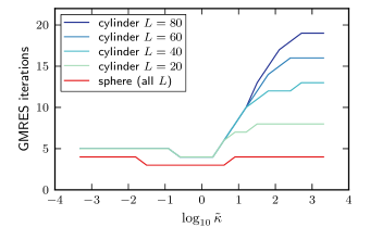
Figure 1: Number of GMRES iterations required to calculate the polarization charge $\sigma_{b}$ on a dielectric cylinder or sphere as a function of the dielectric contrast $\tilde{\kappa}$. We use cylinders with unit radius and different lengths $L$. Convergence is generally reached very quickly, except in geometries with extreme aspect ratios and extreme $\tilde{\kappa}$. The convergence threshold is $||r^{(m)}||<10^{-4}||b||$ [Eq. (59)], where $r^{(m)}=b-\mathcal{A}x^{(m)}$ is the residual of the $m^{\mathrm{th}}$ iterative approximation $x^{(m)}$ to the bound charge $\sigma_{b}$. We observe empirically that our convergence threshold corresponds to a relative error in the electrostatic energy of approximately $10^{-4}$.

In practice, we observe that GMRES finds the bound charge in very few iterations. This observation is supported by mathematical properties of the GMRES algorithm Saad and Schultz (1986). Because $\mathcal{A}$ is positive definite [cf. Eq. (50)], the residual error decreases exponentially with the number of iterations. If $\mathcal{A}$ were also symmetric, then its condition number could be used to bound the rate of GMRES convergence. For our non-symmetric operator, less is known analytically. Here, we demonstrate empirically that the convergence rate is linked to the ratio of extremal values, $\lambda_{\mathrm{ratio}}=\lambda_{\mathrm{max}}/\lambda_{\mathrm{min}}$ [Eq. (51)]. In Sec. III we bounded $\lambda_{\mathrm{ratio}}\leq\kappa_{\mathrm{max}}/\kappa_{\mathrm{min}}$, and estimated $\lambda_{\mathrm{ratio}}$ for sphere, cylinder and slab geometries.

Figure 1 demonstrates the link between fast GMRES convergence and the smallness of $\lambda_{\mathrm{ratio}}$. For a single sphere $\lambda_{\mathrm{ratio}}<3$, and GMRES converges within a handful of iterations regardless of the dielectric contrast $\tilde{\kappa}=\kappa_{\mathrm{obj}}/\kappa_{\mathrm{bg}}$. In molecular dynamics simulations of many spheres in various configurations, we observed GMRES convergence almost identical to that of the single-sphere system Barros and Luijten (2013). The worst-case convergence rates occur in geometries with extreme aspect ratios. For a cylinder, we predict $\lambda_{\mathrm{ratio}}\approx\kappa_{\mathrm{max}}/\kappa_{\mathrm{min}}$ only when $\tilde{\kappa}\gg 1$ and the cylinder length $L$ is much larger than its radius. Indeed, this is precisely the regime where Fig. 1 shows slowed GMRES convergence. We observe that, at fixed accuracy, the number of GMRES iterations scales like $\ln\lambda_{\mathrm{ratio}}$.

IV.7 Treatment of isolated point charges

We allow systems to contain isolated point charges in addition to dielectric objects, a situation that typically occurs in simulations involving ionic solutions. In the bulk of a medium, where the dielectric constant $\kappa(\mathbf{r})=\kappa_{0}$ is uniform, Eq. (25) states that free charges are screened by the factor $\kappa^{-1}_{0}$. In numerics we typically deal with isolated free charges $q_{f}$, to which we must associate a net (free and bound) charge $q_{f}/\kappa_{0}$.

Thus, only the surface bound charge $\sigma_{b}$ on the dielectric objects remains to be calculated. To do so, we solve Eq. (41) with $b$ in Eq. (42) defined via the electric field $\mathbf{E}_{f}$ generated by both free surface charge $\sigma_{f}$ and screened point charges $q_{f}/\kappa_{0}$.

IV.8 Fixing net charge on objects

By Eq. (24), we may also fix the net integrated charge on dielectric objects. In particular, if the object is surrounded by a medium with uniform dielectric constant $\kappa_{\mathrm{bg}}$ and carries total free charge $q$ (counting both internal and surface charges), then the total free and bound charge on the object is $q/\kappa_{\mathrm{bg}}$. In the numerical solution of Eq. (40) we should constrain the total charge of each object to its exact value at every GMRES iteration. The first reason for this is accuracy: errors in the net charge (monopole term) can overwhelm relatively subtle dielectric effects. The second reason is convergence rate: as demonstrated in Appendix B, the net charge on an object may correspond to an outlying eigenvalue of the operator $\mathcal{A}$; eliminating the corresponding eigenvector component may significantly improve $\mathcal{A}$’s condition number. The third reason is consistency: if a finite system is not kept charge neutral, the operators $\mathcal{G}$ and $\mathcal{A}$ become ill-defined.

IV.9 Surface representation of free charge

In addition to fixing the net charge of each object to its exact value during the GMRES iterations, there is another technique to improve accuracy. Typically, the dielectric object and its free charge distribution are rigid. In this case, we care only about the electric field that the free charge produces externally. Thus, we may replace any distribution of internal free charge with an equivalent free charge distribution at the object surface Jackson (1999). If, instead, internal free charge were present, there would be expected (partial) cancellations between the internal charge and the bound surface charge. Small inaccuracies in the Ewald solver would lead to inexact cancellation, a spurious monopole moment, and potentially large numerical error. We avoid such cancellation errors via the surface representation of free charge.

For each charged object, we may calculate the equivalent free surface charge as follows. Consider a virtual system containing the internal free charge, the object medium replaced by vacuum ($\kappa_{\mathrm{obj}}=1$), and the background medium replaced by a conductor ($\kappa_{\mathrm{bg}}\rightarrow\infty$), in which the “virtual” electric field is zero. We use our dielectric method to calculate the bound surface charge for this virtual system [with net charge fixed to zero by Eq. (24)]. By the principle of superposition, the desired free surface charge distribution is then the negative of the calculated virtual bound charge.

IV.10 Bound charge initialization

In a molecular dynamics simulation, dielectric objects move only a small amount during each time step. The bound charge $\sigma_{b}(t-\Delta t)$ that was calculated at the previous time step may be used as the initial guess for $\sigma_{b}(t)$ at the current time step. In our study of interacting dielectric spheresBarros and Luijten (2013) we observed that this optimization reduced the required GMRES iterations per time step from about 4 to 3 when the accuracy target was $10^{-4}$.

IV.11 Direct residual

We save a call to the Ewald solver by avoiding the explicit calculation of $b$. Instead, we compute the residual as

$$r^{(m)} =b-\mathcal{A}x^{(m)}$$

$$=\sigma_{f}-\bar{\kappa}(\sigma_{f}+x^{(m)})-\varepsilon_{0}\Delta\kappa\mathbf{E}^{(m)}\cdot\hat{n}\;.$$ (60)

Here we reuse $\mathbf{E}^{(m)}$ (the electric field due to both free charge $\sigma_{f}$ and estimated bound charge $x^{(m)}$), which GMRES already calculated to construct the Krylov space. We also replace Eq. (59) with a convergence criterion that is independent of $b$, $||r^{(m)}||<10^{-4}|x^{(m)}|c$. We select $c$ to be a “typical” dielectric constant. In a system containing only two types of dielectric media, we choose $c=\bar{\kappa}$, the mean dielectric constant.

IV.12 Energy calculation

Equation (22) suggests calculating the energy in two steps: (1) generate the potential $\psi=\mathcal{G}(\rho_{f}+\rho_{b})/\varepsilon_{0}$ due to free and bound charge, and (2) sum the energy contributions at the locations of free charge, $U=(1/2)\int\rho_{f}\psi\,\mathrm{d}\mathbf{r}$. The surface patch corrections described in Sec. IV.2 naturally extend to the calculation of the potential $\psi_{ij}$ generated by surface patch $j$ and evaluated at surface patch $i$.

Most electrostatics software packages do not provide a procedure to calculate $\psi$. However, these packages can still be used to calculate the dielectric energy efficiently. Our trick is to express the energy as

$$U=\frac{1}{2}({\tilde{U}}_{\mathrm{elec}}[\rho_{f}]-{\tilde{U}}_{\mathrm{elec}}[\rho_{b}]+{\tilde{U}}_{\mathrm{elec}}[\rho_{f}+\rho_{b}])\;,$$ (61)

where ${\tilde{U}}_{\mathrm{elec}}[\tilde{\rho}]$ represents the energy of the electric field generated by the charge density $\tilde{\rho}(\mathbf{r})$ alone,

$${\tilde{U}}_{\mathrm{elec}}[\tilde{\rho}]=\frac{1}{2\varepsilon_{0}}\int_{V}\tilde{\rho}\mathcal{G}\tilde{\rho}\,\mathrm{d}\mathbf{r}\;.$$ (62)

In particular, by Eqs. (3), (5), and (9),

$$U_{\mathrm{elec}}={\tilde{U}}_{\mathrm{elec}}[\rho_{f}+\rho_{b}]$$ (63)

is the bare electric field energy for the physical system.

Equation (61) states that we can calculate the full dielectric energy using three separate calls to an Ewald solver. In typical molecular dynamics applications, the energy is sampled at only a small fraction of the time steps, and the cost of the two extra Ewald evaluations is negligible.

V Comparison with previous numerical methods

V.1 Richardson Iteration

Many existing simulation methods effectively calculate the bound charge by Richardson iteration Richardson (1910), motivating us to consider this case in detail.

The method proposed in Ref. Levitt, 1978 is perhaps the earliest, and it iteratively calculates the surface bound charge $\sigma_{b}=x$ via

$$x^{(m+1)}=-\varepsilon_{0}\frac{\Delta\kappa}{\overline{\kappa}}\mathbf{E}^{(m)}\cdot\hat{n}\;,$$ (64)

where $\mathbf{E}^{(m)}$ is the electric field generated by both non-surface charges and the surface bound charge $x^{(m)}$ from the previous iteration. Zero free surface charge, $\sigma_{f}=0$, is assumed. In the operator notation of Eqs. (41) and (42), the recurrence becomes

$$x^{(m+1)}=x^{(m)}+\gamma(b-\mathcal{A}x^{(m)})\;,$$ (65)

where $\gamma^{-1}=\bar{\kappa}$ is the mean dielectric constant at the surface. This numerical scheme, Richardson iteration, is readily analyzed for arbitrary $\gamma$ Young (1989). After some algebra, we express the residual $r^{(m)}=b-\mathcal{A}x^{(m)}$ as a linear recurrence,

$$r^{(m+1)}=(1-\gamma\mathcal{A})r^{(m)}\;.$$ (66)

To solve this recurrence, we work in the basis of eigenvectors $\{v_{\lambda}\}$ of the operator $\mathcal{A}$. The residual vectors become $r^{(m)}=\sum_{\lambda}r^{(m)}_{\lambda}v_{\lambda}$ and we obtain the solution

$$r^{(m+1)}_{\lambda}=(1-\gamma\lambda)r^{(m)}_{\lambda}=(1-\gamma\lambda)^{m+1}r^{(0)}_{\lambda}\;.$$ (67)

The consequence is that $r^{(m)}$ converges to zero if $|1-\gamma\lambda|<1$ is satisfied for each eigenvalue $\lambda$. Clearly $\gamma$ should be selected according to the spectra of $\mathcal{A}$.

Somewhat remarkably, the implicit choice of Ref. Levitt, 1978, $\gamma=2/(\kappa_{\mathrm{min}}+\kappa_{\mathrm{max}})$, leads to a convergent scheme. The eigenvalue bounds $1\leq\kappa_{\min}\leq\lambda\leq\kappa_{\max}$ of Eq. (50) imply

$$|1-\gamma\lambda|\leq\frac{\kappa_{\mathrm{max}}-\kappa_{\mathrm{min}}}{\kappa_{\mathrm{max}}+\kappa_{\mathrm{min}}}<1\;.$$ (68)

Although this scheme is consistent, other iterative solution methods such as GMRES and BiCGSTAB are preferable for their much faster convergence Saad (2003).

In the method of Ref. Tyagi et al., 2010, Eq. (64) is generalized to

$$x^{(m+1)}=-\omega\varepsilon_{0}\frac{\Delta\kappa}{\overline{\kappa}}\mathbf{E}^{(m)}\cdot\hat{n}+(1-\omega)x^{(m)}\;,$$ (69)

for tunable $\omega$. This scheme again corresponds to Richardson iteration, Eq. (65), now with step size $\gamma=\omega/\bar{\kappa}$.

In a naïve implementation, each Richardson iteration requires $\mathcal{O}(n^{2})$ operations to determine the electric field $\mathbf{E}^{(m)}$ at all $n$ surface patches. As discussed in Sec. IV.4, this cost can be reduced to $\mathcal{O}(n\ln n)$ or $\mathcal{O}(n)$ with a fast Ewald solver.

V.2 Variational approaches

In our review of linear dielectrics, Sec. II, we introduced the equilibrium polarization field as the one minimizing the (free) energy functional $U=U_{\mathrm{elec}}+U_{\mathrm{pol}}$. This variational formulation of dielectrics can be used as the basis of numerical methods Marchi et al. (2001); Levy et al. (2005); Maggs and Everaers (2006); Rottler and Krayenhoff (2009), at the cost of working with the bulk polarization (rather than just the surface bound charge). As we have seen, numerical efficiency is much improved by posing the dielectric problem in terms of bound charge restricted to the dielectric interfaces. Using an alternate variational formulation of the dielectric problem Jackson (1999), the authors of Ref. Allen et al., 2001 determine the bound charge as the distribution that minimizes a given functional. Subsequently, a similar functional was found that, when minimized, corresponds to the energy Jadhao et al. (2012). This latter approach enables Car–Parrinello type molecular dynamics simulation. Here, we analyze the computational efficiency of numerical methods to calculate the bound charge based upon these variational formulations.

The electrostatic energy may be expressed as the extremum of the functional Jadhao et al. (2012)

$$\mathcal{U}[\mathbf{P},\rho_{b},\psi]=U-\int_{V}\psi(\mathbf{r})[\rho_{b}(\mathbf{r})+\nabla\cdot\mathbf{P}(\mathbf{r})]\,\mathrm{d}\mathbf{r}\;.$$ (70)

The Lagrange multiplier $\psi(\mathbf{r})$ in Eq. (70) enforces the physical constraint $\nabla\cdot\mathbf{P}=-\rho_{b}$. By Eqs. (8), (63) and (10) the electrostatic energy $U=U_{\mathrm{elec}}+U_{\mathrm{pol}}$ has the functional form

$$U=\frac{1}{2\varepsilon_{0}}\int_{V}\left[(\rho_{f}+\rho_{b})\mathcal{G}(\rho_{f}+\rho_{b})+\frac{\mathbf{P}^{2}}{\kappa-1}\right]\,\mathrm{d}\mathbf{r}\;.$$ (71)

From $\mathcal{U}$, we wish to construct new functionals that are independent of $\mathbf{P}$ and $\psi$, and that are still extremized by the physical bound charge $\rho_{b}$. We extremize $\mathcal{U}$ with respect to $\rho_{b}$ and $\mathbf{P}$, and obtain

$$\psi =\mathcal{G}(\rho_{f}+\rho_{b})/\varepsilon_{0}\;,$$ (72)

$$\mathbf{P} =-(\kappa-1)\nabla\mathcal{G}(\rho_{f}+\rho_{b})\;.$$ (73)

Substitution of Eqs. (72) and (73) into $\mathcal{U}$ yields the negative of the functional considered in Ref. Allen et al., 2001,

$$\mathcal{I}[\rho_{b}]=\frac{1}{2}\int_{V}\left[\rho_{f}\mathcal{G}(\rho_{f}+R_{b}[\rho_{b}])-\rho_{b}\mathcal{G}(\rho_{b}-R_{b}[\rho_{b}])\right]\,\mathrm{d}\mathbf{r}\;,$$ (74)

where

$$R_{b}=\nabla\cdot(\kappa-1)\nabla\mathcal{G}(\rho_{f}+\rho_{b})=(1-\mathcal{A})(\rho_{f}+\rho_{b})\;.$$ (75)

We may also extremize $\mathcal{U}$ with respect to $\psi$, in which case $\rho_{b}=R_{b}[\rho_{b}]$. Partial substitution then yields the alternate functional introduced in Ref. Jadhao et al., 2012,

$$\mathcal{J}[\rho_{b}]=\frac{1}{2}\int_{V}\left[\rho_{f}\mathcal{G}(\rho_{f}+R_{b}[\rho_{b}])-R_{b}[\rho_{b}]\mathcal{G}(\rho_{b}-R_{b}[\rho_{b}])\right]\,\mathrm{d}\mathbf{r}\;,$$ (76)

The variation of $\mathcal{I}[\rho_{b}]$ and $\mathcal{J}[\rho_{b}]$ is readily calculated using the identities

$$\int_{V}f\mathcal{G}\frac{\delta\rho_{b}}{\delta\rho_{b}}\,\mathrm{d}\mathbf{r} =\mathcal{G}f\;,$$ (77)

$$\int_{V}f\mathcal{G}\frac{\delta R_{b}}{\delta\rho_{b}}\,\mathrm{d}\mathbf{r} =\mathcal{G}(1-\mathcal{A})f\;,$$ (78)

valid for any test function $f(\mathbf{r})$. Extremization then yields

$$\frac{\delta\mathcal{I}}{\delta\rho_{b}} =\mathcal{G}(b-\mathcal{A}\rho_{b})=0\;,$$ (79)

$$\frac{\delta\mathcal{J}}{\delta\rho_{b}} =\mathcal{G}(1-\mathcal{A})(b-\mathcal{A}\rho_{b})=0\;,$$ (80)

which are uniquely satisfied when $\mathcal{A}\rho_{b}=b$ [Eq. (19)], thus giving the correct bound charge.

Reference Allen et al., 2001 calculates $x=\rho_{b}$ by a steepest-ascent procedure,

$$x^{(m+1)}=x^{(m)}+\mathcal{\gamma}\frac{\delta\mathcal{I}}{\delta x^{(m)}}=x^{(m)}+\gamma\mathcal{G}(b-\mathcal{A}x^{(m)})\;,$$ (81)

where $\gamma$ is a step size parameter. We recognize this variational scheme as Richardson iteration, Eq. (65), preconditioned by the positive definite operator $\mathcal{G}$. By Eq. (67), the convergence rate of Richardson iteration is controlled by the ratio of extremal eigenvalues, $\lambda_{\mathrm{ratio}}=|\lambda_{\max}/\lambda_{\min}|$, of the relevant operator—in this case $\mathcal{GA}$.

We demonstrated in Sec. III that $\mathcal{A}$ is well conditioned. In contrast, the eigenvalues of $\mathcal{G}\mathcal{A}$ are unbounded in the continuum limit of small patches—the operator has infinite condition number. We use simple scaling to compare the spectra of $\mathcal{A}$ and $\mathcal{GA}$. The operator $\mathcal{A}$ is dimensionless and its eigenvalues are independent of length scale. Since $\mathcal{G}$ is inverse to $\nabla^{2}$, it has dimensions of length squared. The operator $\mathcal{GA}$ inherits these dimensions. Thus, eigenvectors of $\mathcal{G}\mathcal{A}$ with characteristic frequency $k$ have eigenvalues that scale as $k^{-2}$. In the continuum limit, arbitrarily small eigenvalues are possible. As a concrete example, consider the uniform dielectric system $\kappa(\mathbf{r})=\kappa_{\mathrm{bg}}$ where $\mathcal{A=\kappa_{\mathrm{bg}}}$. The eigenvectors of $\mathcal{GA=\kappa_{\mathrm{bg}}G}$ are the Fourier modes $\exp(i\mathbf{k}\cdot\mathbf{r})$ with eigenvalues $\kappa_{\mathrm{bg}}|k|^{-2}$ ranging from $0$ to $\infty$.

In practice, the largest $k$-vector is cut off by the inter-patch distance length scale. Similarly, the smallest $k$-vector is set by the scale of the largest dielectric objects. Nonetheless, $\mathcal{GA}$ is unnecessarily ill-conditioned. Thus the scheme of Eq. (81) requires many iterations for the bound charge to converge.

These scaling considerations also apply to variational methods based on $\mathcal{J}[\rho_{b}]$. Unlike $\mathcal{I}[\rho_{b}]$, the functional $\mathcal{J}[\rho_{b}]$ may be interpreted as an effective energy functional in the sense that

$$\min_{\rho_{b}}\mathcal{J}[\rho_{b}]=U\;,$$ (82)

where $U$ is the usual dielectric energy. Reference Jadhao et al., 2012 applied Car–Parrinello molecular dynamics to evolve $\rho_{b}$ along with ion positions according to the Hamiltonian $\mathcal{J}$ Car and Parrinello (1985). An artificially low temperature was separately applied to the $\rho_{b}$ degrees of freedom. Thus, $\rho_{b}$ was effectively solved by the overdamped dynamics,

$$\frac{\partial\rho_{b}(\mathbf{r})}{\partial t}=-\gamma\frac{\delta\mathcal{J}}{\delta\rho_{b}(\mathbf{r})}\;,$$ (83)

for which we recover Eq. (81) but now with $\mathcal{G}(1-\mathcal{A})\mathcal{A}$ as the relevant operator. As before, dimensional analysis tells us that $\mathcal{G}(1-\mathcal{A})\mathcal{A}$ is ill-conditioned, and that $\rho_{b}$ will converge slowly. In practice, this means that a very small Car–Parrinello molecular dynamics time step must be employed.

V.3 Induced Charge Computation (ICC) method

The ICC method Boda et al. (2004) proposed to solve Eq. (40) by explicit construction of the matrix inverse $\mathcal{A}^{-1}$. Direct matrix inversion costs $\mathcal{O}(n^{3})$ for $n$ surface patch elements. Subsequently, the bound charge $x=\sigma_{b}$ may be found by dense matrix–vector multiplication, $x=\mathcal{A}^{-1}b$, where $b$ is a function of the evolving free charge. For static dielectric geometries, each evaluation of $x$ then costs $\mathcal{O}(n^{2})$, which is much worse than $\mathcal{O}(n)$ methods based upon fast Ewald solvers. If the dielectric geometry dynamically evolves, then repeated matrix inversion is required, for which the authors of Ref. Boda et al., 2004 suggested GMRES as an alternative.

V.4 GMRES with fast matrix–vector product

In light of the drawbacks of previously proposed methods, namely the use of inefficient iterative methods employing Richardson iteration (Sec. V.1), an ill-conditioned operator and hence poor convergence rates of variational methods (Sec. V.2), and inefficient matrix–vector multiplication (and moreover matrix inversion) for the ICC method (Sec. V.3), we advocate calculation of the bound charge by solving Eq. (40) via GMRES and a fast Ewald solver. With this approach, the surface bound charge converges to high accuracy in only a handful of GMRES iterations, each requiring $\mathcal{O}(n)$ or $\mathcal{O}(n\ln n)$ operations, depending on the Ewald solver used.

During the preparation of this publication, it came to our attention that our strategy was proposed already in Ref. Bharadwaj et al., 1995, which has been overlooked and underappreciated, as evidenced by the wide array of subsequent methods proposals. We note, however, that due to the large number of patches typically introduced for each dielectric object, the acceleration techniques introduced in Sections IV.8–IV.11 are still instrumental in realizing dynamic simulations such as those of Ref. Barros and Luijten, 2013.

VI Summary

In this paper we have demonstrated a collection of techniques by which dynamic dielectric systems can be simulated efficiently. In geometries with sharp dielectric boundaries, one solves a matrix equation to obtain the surface bound charge, from which energy and forces follow directly. Empirically, we find that the bound charge converges to high accuracy after a handful of GMRES iterations. We attribute this fast convergence to the compact spectrum of the relevant operator $\mathcal{A}$, whose properties we have analyzed in detail. Each iteration of GMRES requires only a single calculation of the electric field in vacuum, which can be performed with an Ewald solver at a cost that scales nearly linearly in the number of surface patch elements $n$.

Compared to several previous methods, our approach (i) converges quickly, by using GMRES rather than Richardson iteration Levitt (1978); Hoyles et al. (1998); Tyagi et al. (2010), (ii) avoids the ill-conditioned matrix equations of variational approaches Allen et al. (2001); Jadhao et al. (2012), (iii) does not require explicit construction of the matrix inverse Boda et al. (2004), and (iv) evaluates matrix–vector products very efficiently with a fast Ewald solver. A side benefit of (iv) is that we properly treat periodic geometries common in computational studies. To illustrate the capabilities of our method, we have performed the first large-scale simulation of dynamical dielectric objects in Ref. Barros and Luijten, 2013.

Appendix A Dielectric forces

We derive forces in dielectric systems as a sum of pairwise Coulomb-like interactions between free and bound charges. We follow the approach advocated in Ref. Landau et al., 1993 and carried out in Refs. Schwinger et al., 1998; Zangwill, 2013. That is, we derive the force on a dielectric object as the energy derivative with respect to object motion.

Our first task is to express the electric field and energy as a function of $\rho_{f}(\mathbf{r})$ and $\kappa(\mathbf{r})$ alone. Combining Eqs. (17) and (18) we obtain

$$\varepsilon_{0}\psi=\mathcal{G}(\rho_{f}+\rho_{b})=(-\nabla\cdot\kappa\nabla)^{-1}\rho_{f}\;.$$ (84)

The existence of the symmetric operator $(\nabla\cdot\kappa\nabla)^{-1}$ follows from the existence of the potential $\psi$. The electric field $\mathbf{E}=-\nabla\psi$ immediately follows,

$$\mathbf{E}=\frac{1}{\varepsilon_{0}}\nabla(\nabla\cdot\kappa\nabla)^{-1}\rho_{f}\;.$$ (85)

The energy in Eq. (22) becomes a nonlocal, $\kappa(\mathbf{r})$-dependent sum of free charge pairs,

$$U=-\frac{1}{2\varepsilon_{0}}\int\rho_{f}(\nabla\cdot\kappa\nabla)^{-1}\rho_{f}\,\mathrm{d}\mathbf{r}\;.$$ (86)

A.1 Force on free charge

The force density $\mathbf{f}$ associated with displacement of the free charge $\rho_{f}$ at position $\mathbf{r}$ in any direction $\hat{\mathbf{n}}$ is given by

$$\hat{\mathbf{n}}\cdot\mathbf{f}=-\lim_{\varepsilon\rightarrow 0}\frac{U[\rho_{f}+\varepsilon\rho_{d}]-U[\rho_{f}]}{\varepsilon}\;,$$ (87)

where the displacement distribution is

$$\rho_{d}(\mathbf{r}^{\prime})=\rho_{f}(\mathbf{r})\frac{\delta(\mathbf{r}+\varepsilon\hat{\mathbf{n}}-\mathbf{r}^{\prime})-\delta(\mathbf{r}-\mathbf{r}^{\prime})}{\varepsilon}\;.$$ (88)

We expand in powers of $\varepsilon$, dropping $\mathcal{O}(\varepsilon)$ terms,

$$\frac{U[\rho_{f}+\varepsilon\rho_{d}]-U[\rho_{f}]}{\varepsilon} \approx\int\frac{\delta U}{\delta\rho_{f}(\mathbf{r}^{\prime})}\rho_{d}(\mathbf{r}^{\prime})\,\mathrm{d}\mathbf{r}^{\prime}$$

$$\approx\rho_{f}\hat{\mathbf{n}}\cdot\nabla\frac{\delta U}{\delta\rho_{f}}\;.$$ (89)

The equality becomes exact in the limit $\varepsilon\rightarrow 0$,

$$\mathbf{f}=-\rho_{f}\nabla\frac{\delta U}{\delta\rho_{f}}\;.$$ (90)

Using both Eq. (85) and Eq. (86), we evaluate

$$\mathbf{f}=\frac{\rho_{f}}{\varepsilon_{0}}\nabla(\nabla\cdot\kappa\nabla)^{-1}\rho_{f}=\rho_{f}\mathbf{E}\;.$$ (91)

The net force to move the charge $\rho_{f}(\mathbf{r})$ in a region $\Omega$ is

$$\mathbf{F}_{\mathrm{charge}}=\int_{\Omega}\rho_{f}\mathbf{E}\,\mathrm{d}\mathbf{r}\;.$$ (92)

In particular, the force on a point charge $\rho_{f}(\mathbf{r})=q\delta(\mathbf{r}-\mathbf{r}_{i})$ is simply $q\mathbf{E}$.

A.2 Force on dielectric object

Dielectric object motion affects the energy through changes in $\kappa(\mathbf{r})$. If the background has fixed $\kappa_{\mathrm{bg}}$, then dielectric object motion corresponds to a displacement of $\kappa(\mathbf{r})-\kappa_{\mathrm{bg}}$ at each $\mathbf{r}$. Analogous to Eq. (90), the force density for this displacement is

$$\mathbf{f}=-(\kappa-\kappa_{\mathrm{bg}})\nabla\frac{\delta U}{\delta\kappa}\;.$$ (93)

We will use the identity

$$\frac{\delta}{\delta\kappa}\mathcal{B}^{-1}=-\mathcal{B}^{-1}\frac{\delta\mathcal{B}}{\delta\kappa}\mathcal{B}^{-1}\;,$$ (94)

which is a consequence of the product rule,

$$0=\frac{\delta}{\delta\kappa}(\mathcal{B}\mathcal{B}^{-1})=\frac{\delta\mathcal{B}}{\delta\kappa}\mathcal{B}^{-1}+\mathcal{B}\frac{\delta\mathcal{B}^{-1}}{\delta\kappa}\;.$$ (95)

Note that the operators $\mathcal{B}^{-1}$ and $\delta\mathcal{B}/\delta\kappa$ do not generally commute.

Taking $\mathcal{B}=\nabla\cdot\kappa\nabla$, the functional derivative of the energy, Eq. (86), evaluates to

$$\frac{\delta U}{\delta\kappa} =+\frac{1}{2\varepsilon_{0}}\int_{\Omega}\rho_{f}\mathcal{B}^{-1}\frac{\delta\mathcal{B}}{\delta\kappa}\mathcal{B}^{-1}\rho_{f}\,\mathrm{d}\mathbf{r}$$

$$=-\frac{\varepsilon_{0}}{2}\int_{\Omega}\mathbf{E}\cdot\frac{\delta\kappa}{\delta\kappa}\mathbf{E}\,\mathrm{d}\mathbf{r}$$

$$=-\frac{\varepsilon_{0}}{2}\mathbf{E}^{2}\;.$$ (96)

The minus sign appears after integrating by parts.

In index notation, where repeated indices denote summation, the $\alpha^{\mathrm{th}}$ component of the force per volume is

$$f_{\alpha} =\frac{\varepsilon_{0}}{2}(\kappa-\kappa_{\mathrm{bg}})\partial_{\alpha}E_{\beta}E_{\beta}$$

$$=\varepsilon_{0}(\kappa-\kappa_{\mathrm{bg}})E_{\beta}\partial_{\alpha}E_{\beta}\;.$$ (97)

The electric field is a gradient, $E_{\beta}=-\partial_{\beta}\psi$, so it follows that $\partial_{\alpha}E_{\beta}=\partial_{\beta}E_{\alpha}$ and

$$f_{\alpha} =\varepsilon_{0}(\kappa-\kappa_{\mathrm{bg}})E_{\beta}\partial_{\beta}E_{\alpha}$$

$$=\varepsilon_{0}\partial_{\beta}[(\kappa-\kappa_{\mathrm{bg}})E_{\beta}E_{\alpha}]-\varepsilon_{0}[\partial_{\beta}(\kappa-\kappa_{\mathrm{bg}})E_{\beta}]E_{\alpha}\;.$$ (98)

Equivalently,

$$\mathbf{f}=\varepsilon_{0}\nabla\cdot[(\kappa-\kappa_{\mathrm{bg}})\mathbf{E}\otimes\mathbf{E}]-\varepsilon_{0}[\nabla\cdot(\kappa-\kappa_{\mathrm{bg}})\mathbf{E}]\mathbf{E}\;.$$ (99)

From Eqs. (1) and (16) we have

$$\nabla\cdot(\kappa-\kappa_{\mathrm{bg}})\mathbf{E} =\nabla\cdot\kappa\mathbf{E}-\kappa_{\mathrm{bg}}\nabla\cdot\mathbf{E}$$

$$=\frac{1}{\varepsilon_{0}}[\rho_{f}-\kappa_{\mathrm{bg}}(\rho_{f}+\rho_{b})]\;,$$ (100)

yielding

$$\mathbf{f}=\varepsilon_{0}\nabla\cdot[(\kappa-\kappa_{\mathrm{bg}})\mathbf{E}\otimes\mathbf{E}]+[\kappa_{\mathrm{bg}}(\rho_{f}+\rho_{b})-\rho_{f}]\mathbf{E}\;.$$ (101)

The net dielectric force, $\mathbf{F}_{\mathrm{diel}}=\int_{\Omega}\mathbf{f}\,\mathrm{d}\mathbf{r}$, is an integral over a region $\Omega$ enclosing the object and its surface. After applying Gauss’s theorem, the total force separates into a boundary term $\varepsilon_{0}\int_{\partial\Omega}(\kappa-\kappa_{\mathrm{bg}})(\hat{n}\cdot\mathbf{E})\mathbf{E}\,\mathrm{d}\mathbf{s}$ and a bulk term $\int_{\Omega}[\kappa_{\mathrm{bg}}(\rho_{f}+\rho_{b})-\rho_{f}]\mathbf{E}\,\mathrm{d}\mathbf{r}$. The boundary term is zero because, by construction, the integral is evaluated where $\kappa(\mathbf{r})=\kappa_{\mathrm{bg}}$. The net dielectric force on the object becomes

$$\mathbf{F}_{\mathrm{diel}}=\int_{\Omega}[\kappa_{\mathrm{bg}}(\rho_{f}+\rho_{b})-\rho_{f}]\mathbf{E}\,\mathrm{d}\mathbf{r}\;,$$ (102)

where $\rho_{f}$ has been treated as fixed.

Typically, free charge moves rigidly with the object, so we should also include its force, Eq. (92). The total force on the dielectric object is then

$$\mathbf{F}=\mathbf{F}_{\mathrm{charge}}+\mathbf{F}_{\mathrm{diel}}=\kappa_{\mathrm{bg}}\int_{\Omega}(\rho_{f}+\rho_{b})\mathbf{E}\,\mathrm{d}\mathbf{r}\;.$$ (103)

As a consistency check, note that in the special case where $\kappa(\mathbf{r})=\kappa_{\mathrm{bg}}$ is constant, we have $(\rho_{f}+\rho_{b})=\rho_{f}/\kappa_{\mathrm{bg}}$ and the dielectric force is zero, $\mathbf{F}_{\mathrm{diel}}=\mathbf{0}$.

Appendix B Exact spectra for simple geometries

For certain dielectric geometries the entire spectrum of $\mathcal{A}$ can be determined. The key observation is that the eigenvectors of $\mathcal{A}$ coincide with the solutions of the Laplace equation $\nabla^{2}\psi=0$ in non-Cartesian coordinates, when those solutions are separable in the normal component. This solution technique applies to the dielectric sphere, cylinder, and slab. In these geometries, $\mathcal{A}$ becomes a symmetric operator.

We seek eigenvectors $\rho$ and eigenvalues $\lambda$ that satisfy $\mathcal{A}\rho=\lambda\rho$. We work with surface charge density $\sigma$, for which Eq. (41) states

$$\mathcal{A}\sigma=\bar{\kappa}\sigma+\Delta\kappa\mathbf{E}\cdot\hat{n}=\lambda\sigma\;,$$ (104)

with $\mathbf{E}=(\mathbf{E}_{\mathrm{out}}+\mathbf{E}_{\mathrm{in}})/2$ the electric field at the surface. We also have $\Delta\kappa=\kappa_{\mathrm{out}}-\kappa_{\mathrm{in}}$, and $\bar{\kappa}=(\kappa_{\mathrm{out}}+\kappa_{\mathrm{in}})/2$. In this section we use dimensionless units where $\varepsilon_{0}=1$.

B.0.1 Sphere

Consider a single spherical object of radius $R$. We work in spherical coordinates $(r,\theta,\phi)$. The operator $\mathcal{A}$ is fixed upon the specification

$$\kappa(r)=\left\{\begin{array}[]{ll}\kappa_{\mathrm{in}}&\mathrm{if}\,\,r<R\\ \kappa_{\mathrm{out}}&\mathrm{if}\,\,r>R\end{array}\right.\;.$$ (105)

The spherical harmonics $Y_{lm}(\theta,\phi)$ form an orthogonal basis for the surface of the sphere. We will demonstrate that the spherical harmonics are in fact the eigenvectors of $\mathcal{A}$. In anticipation of this result, consider the surface charge distribution,

$$\sigma(\theta,\phi)=Y_{lm}(\theta,\phi)\;.$$ (106)

The electrostatic potential due to $\sigma$ is

$$\psi(r,\theta,\phi)=\left\{\begin{array}[]{ll}\psi_{1}=ar^{l}Y_{lm}&\mathrm{if}\,\,r<R\\ \psi_{2}=br^{-l-1}Y_{lm}&\mathrm{if}\,\,r>R\end{array}\right.\;,$$ (107)

where

$$a =\frac{\sigma_{0}}{2l+1}R^{-l+1}\;,$$ (108)

$$b =\frac{\sigma_{0}}{2l+1}R^{l+2}\;.$$ (109)

As required, $\psi$ satisfies the Laplace equation $\nabla^{2}\psi=0$ for $r\neq R$, and obeys appropriate boundary conditions at $r=R$:

$$\psi_{2}-\psi_{1}|_{r=R} =0\;,$$ (110)

$$\partial_{r}\psi_{2}-\partial_{r}\psi_{1}|_{r=R} =-\sigma\;.$$ (111)

The electric field projected onto the surface normal is

$$\hat{r}\cdot\mathbf{E}=-\frac{(\partial_{r}\psi_{1}+\partial_{r}\psi_{2})}{2}=-\frac{\sigma}{2(2l+1)}[-(l+1)+l]\;.$$ (112)

Comparison with Eq. (104) confirms that $\sigma$ is indeed an eigenvector,

$$\mathcal{A\sigma}=\lambda\sigma =\bar{\kappa}\sigma+\Delta\kappa\mathbf{E}\cdot\hat{r}$$

$$=\left(\bar{\kappa}+\frac{\Delta\kappa}{2(2l+1)}\right)\sigma\;.$$ (113)

Expanding $\bar{\kappa}=(\kappa_{\mathrm{out}}+\kappa_{\mathrm{in}})/2$ and $\Delta\kappa=\kappa_{\mathrm{out}}-\kappa_{\mathrm{in}}$ we get

$$\lambda=\left\{\kappa_{\mathrm{out}},\left(\frac{2}{3}\kappa_{\mathrm{out}}+\frac{1}{6}\kappa_{\mathrm{in}}\right),\ldots,\left(\frac{1}{2}\kappa_{\mathrm{out}}+\frac{1}{2}\kappa_{\mathrm{in}}\right)\right\}\;.$$ (114)

The eigenvalue $\lambda=\kappa_{\mathrm{out}}$ corresponds to the eigenvector of uniform surface charge, $Y_{l=0,m=0}$. In a numerical implementation, we constrain the net surface charge to its exact value as described in Sec. IV.8, effectively eliminating this eigenvector from the space. The eigenvalue $\lambda=\kappa_{\mathrm{out}}$ should therefore be ignored.

The ratio $\lambda_{\mathrm{ratio}}=\lambda_{\max}/\lambda_{\min}$ is greatest when $\kappa_{\mathrm{out}}\gg\kappa_{\mathrm{in}}$ or $\kappa_{\mathrm{in}}\gg\kappa_{\mathrm{out}}$, where $\lambda_{\mathrm{ratio}}\approx 4/3$ or $3$, respectively.

B.0.2 Cylinder

We now adopt cylindrical coordinates $(\rho,\theta,z)$ and consider a dielectric cylinder,

$$\kappa(\rho)=\left\{\begin{array}[]{ll}\kappa_{\mathrm{in}}&\mathrm{if}\,\,\rho<R\\ \kappa_{\mathrm{out}}&\mathrm{if}\,\,\rho>R\end{array}\right.\;.$$ (115)

We will show that the eigenvectors of $\mathcal{A}$ take the form

$$\sigma=e^{ikz+i\nu\theta}$$ (116)

for real wave number $k$ and integer wave number $\nu$. The functions $\sigma(z,\theta)$ are the Fourier modes of the cylinder surface and form a complete basis.

The electrostatic potential for $\sigma$ is

$$\psi(\rho,\theta,z)=\left\{\begin{array}[]{ll}\psi_{1}&\mathrm{if}\,\,\rho<R\\ \psi_{2}&\mathrm{if}\,\,\rho>R\end{array}\right.\;,$$ (117)

where

$$\psi_{1} =[aK_{\nu}(kR)]I_{\nu}(k\rho)e^{ikz+i\nu\theta}\;,$$ (118)

$$\psi_{2} =[aI_{\nu}(kR)]K_{\nu}(k\rho)e^{ikz+i\nu\theta}\;,$$ (119)

$$a =-\frac{1}{k}\left[I_{\nu}(kR)K_{\nu}^{\prime}(kR)-I_{\nu}^{\prime}(kR)K_{\nu}(kR)\right]{}^{-1}\;.$$ (120)

$I_{\nu}$ and $K_{\nu}$ are the modified Bessel functions of the first and second kind, and primes denote derivatives: $I_{\nu}^{\prime}(x)=\,\mathrm{d}I(x)/\,\mathrm{d}x$ and $K_{\nu}^{\prime}(x)=\,\mathrm{d}K(x)/\,\mathrm{d}x$. As required, $\psi$ satisfies the Laplace equation $\nabla^{2}\psi=0$ for $\rho\neq R$ and obeys appropriate boundary conditions at $\rho=R$,

$$\psi_{2}-\psi_{1}|_{\rho=R} =0\;,$$ (121)

$$\partial_{\rho}\psi_{2}-\partial_{\rho}\psi_{1}|_{\rho=R} =-\sigma\;.$$ (122)

The induced electric field projected onto the surface normal is

$$\mathbf{E}\cdot\hat{\rho} =-\frac{(\partial_{\rho}\psi_{1}+\partial_{\rho}\psi_{2})|_{\rho=R}}{2}$$

$$=\frac{1}{2}\left(\frac{1+C}{1-C}\right)\sigma\;,$$ (123)

where

$$C(\nu,kR)=\frac{I_{\nu}^{\prime}(kR)K_{\nu}(kR)}{I_{\nu}(kR)K_{\nu}^{\prime}(kR)}\;.$$ (124)

Comparison with Eq. (104) confirms that $\sigma$ is indeed an eigenvector, with eigenvalue

$$\lambda=\bar{\kappa}+\frac{\Delta\kappa}{2}\frac{1+C}{1-C}\;.$$ (125)

The eigenvalues $\lambda$ are determined by the function $C(\nu,kR)$, which satisfies $-1\leq C\leq 0$. The maximum of $C$ occurs at low-frequency modes: $C\rightarrow 0$ when $\nu=0$ and $kR\rightarrow 0$. Conversely, $C\rightarrow-1$ for high frequencies $kR\rightarrow\infty$. The extreme eigenvalues follow immediately,

$$\lambda\rightarrow\left\{\begin{array}[]{ll}\bar{\kappa}+\frac{1}{2}\Delta\kappa=\kappa_{\mathrm{out}}&\mathrm{if}\,\,(\nu=0,kR\rightarrow 0)\\ \bar{\kappa}=\frac{1}{2}(\kappa_{\mathrm{out}}+\kappa_{\mathrm{in}})&\mathrm{if}\,\,kR\rightarrow\infty\end{array}\right.\;.$$ (126)

The ratio $\lambda_{\mathrm{ratio}}=\lambda_{\max}/\lambda_{\min}$ is greatest when $\kappa_{\mathrm{in}}\gg\kappa_{\mathrm{out}}$, where $\lambda_{\mathrm{ratio}}\approx\kappa_{\mathrm{in}}/(2\kappa_{\mathrm{out}})$. In the limit $\kappa_{\mathrm{out}}\gg\kappa_{\mathrm{in}}$ we find $\lambda_{\mathrm{ratio}}\approx 2$.

If the length of the cylinder $L$ is not too much greater than the radius $R$, then $\lambda_{\mathrm{ratio}}$ can be reasonable even in the limit $\kappa_{\mathrm{in}}\gg\kappa_{\mathrm{out}}$. For finite $L$, we ignore fringe effects and assume that the above analysis is approximately correct with axial wave numbers taking discrete values $k=\frac{2\pi}{L}\{0,1,\ldots\}$. As in the spherical case, the zeroth mode represents a uniform charge distribution, and can be manually removed from the vector space. If $L/R$ is not too large then $C(\nu=0,kR\ll 1)$ deviates significantly from $0$, increasing the associated eigenvalue. For example, if we choose $L/R=30$ and $k=2\pi/L$ then $C(0,kR)\approx-0.039$. Assuming $\kappa_{\mathrm{in}}\gg\kappa_{\mathrm{out}}$, the smallest eigenvalue is approximately $0.038\kappa_{\mathrm{in}}$, yielding $\lambda_{\mathrm{ratio}}\approx 13.3$ (independent of the ratio $\kappa_{\mathrm{in}}/\kappa_{\mathrm{out}}$).

B.0.3 Slab

The final case to be considered is the slab, where we adopt cartesian coordinates $(x,y,z)$ and choose

$$\kappa(\rho)=\left\{\begin{array}[]{ll}\kappa_{\mathrm{in}}&\mathrm{if}\,\,|z|<R\\ \kappa_{\mathrm{out}}&\mathrm{if}\,\,|z|>R\end{array}\right.\;.$$ (127)

The eigenvectors of $\mathcal{A}$ will be defined by their surface densities on the two planes $z=\pm R$. There are two classes of eigenvectors, symmetric and antisymmetric, represented as

$$\sigma(x,y,R)=\pm\sigma(x,y,-R)=e^{ik_{x}x+ik_{y}y}\;.$$ (128)

The eigenvectors are complete: an arbitrary distribution of charge on both planes can be represented in the basis of symmetric and antisymmetric eigenvectors. The electrostatic potential in the symmetric case is

$$\psi_{s}(x,y,z)=\left\{\begin{array}[]{ll}b_{s}\sigma e^{\gamma z}&\mathrm{if}\,\,z<-R\\ a\sigma\cosh(\gamma z)&\mathrm{if}\,\,|z|<R\\ b_{s}\sigma e^{-\gamma z}&\mathrm{if}\,\,z>+R\end{array}\right.\;,$$ (129)

and for the antisymmetric case,

$$\psi_{a}(x,y,z)=\left\{\begin{array}[]{ll}-b_{a}\sigma e^{\gamma z}&\mathrm{if}\,\,z<-R\\ a\sigma\sinh(\gamma z)&\mathrm{if}\,\,|z|<R\\ b_{a}\sigma e^{-\gamma z}&\mathrm{if}\,\,z>+R\end{array}\right.\;,$$ (130)

where

$$a =\frac{e^{-\gamma R}}{\gamma}\;,$$ (131)

$$b_{s} =\frac{\cosh(\gamma R)}{\gamma}\;,$$ (132)

$$b_{a} =\frac{\sinh(\gamma R)}{\gamma}\;,$$ (133)

$$\gamma =\sqrt{k_{x}^{2}+k_{y}^{2}}\;.$$ (134)

As required, $\psi_{s}$ and $\psi_{a}$ satisfy the Laplace equation in the bulk, and the usual boundary conditions at $z=\pm R$. The induced electric fields at $z=R$, projected onto $\hat{z}$, are

$$\hat{z}\cdot\mathbf{E}=\pm\frac{1}{2}\exp(-2\gamma R)\sigma\;,$$ (135)

where $\pm$ refers to symmetric and antisymmetric eigenvectors, respectively. Comparison with Eq. (104) confirms that the $\sigma$ (symmetric and antisymmetric) are indeed eigenvectors with eigenvalues,

$$\lambda=\bar{\kappa}\pm\frac{\Delta\kappa}{2}\exp(-2\gamma R)\;.$$ (136)

In the high-frequency limit ($k_{x}^{2}+k_{y}^{2}\rightarrow\infty$) the constant $\gamma$ diverges and the eigenvalues tend to $\lambda\rightarrow\kappa=(\kappa_{\mathrm{out}}+\kappa_{\mathrm{in}})/2$. In the opposite limit, where the two planes each have nearly uniform charge, the eigenvalues tend to $\lambda\rightarrow\kappa_{\mathrm{out}}$ and $\kappa_{\mathrm{in}}$ for symmetric and antisymmetric cases, respectively. In these limits, $\lambda_{\mathrm{ratio}}=\kappa_{\max}/\kappa_{\min}$, realizing the worst-case behavior allowed by the bounds of Eq. (50)!

Appendix C Dielectric energies for simple geometries

In Appendix B we studied the exact spectra of a dielectric sphere, cylinder, and slab, and found that $\mathcal{A}$ is generally well-conditioned, except for extreme dielectric contrasts ($\kappa_{\mathrm{in}}\ll\kappa_{\mathrm{out}}$ or $\kappa_{\mathrm{out}}\ll\kappa_{\mathrm{out}}$) in the extended cylinder or slab geometries. Here we demonstrate that, in geometries where $\mathcal{A}$ remains well-conditioned, the energetics saturates quickly as a function of the dielectric contrast.

The scaled energies of a point charge $q$ interacting with dielectric sphere, cylinder, and slab objects are Iversen et al. (1998); Cui (2006),

$$\frac{U_{\mathrm{sphere}}}{u_{0}} =2\frac{d}{r_{0}}\sum_{n=0}^{\infty}\frac{(1-\tilde{\kappa})n(1+d/r_{0})^{-2(n+1)}}{(1+\tilde{\kappa})n+1}\;,$$ (137)

$$\frac{U_{\mathrm{cylinder}}}{u_{0}} =-\frac{8}{\pi}\frac{d}{r_{0}}\int_{0}^{\infty}\left(\frac{1}{2}a_{0}(u)+\sum_{n=1}^{\infty}a_{n}(u)\right)\,\mathrm{d}u;\,\,\,\,\,\,a_{n}(u)=\frac{(1-\tilde{\kappa})K_{n}^{2}((1+d/r_{0})u)}{\tilde{\kappa}\frac{K_{n}(u)}{I_{n}(u)}-\frac{\partial_{u}K_{n}(u)}{\partial_{u}I_{n}(u)}}\;,$$ (138)

$$\frac{U_{\mathrm{slab}}}{u_{0}} =\frac{1-\tilde{\kappa}}{1+\tilde{\kappa}}-\frac{4\tilde{\kappa}}{(1+\tilde{\kappa})^{2}}\sum_{n=1}^{\infty}\left(\frac{1-\tilde{\kappa}}{1+\tilde{\kappa}}\right)^{2n-1}\left(1+\frac{2n}{d/r_{0}}\right)^{-1}\;,$$ (139)

where $r_{0}$ is the radius of the dielectric object (for the slab, $r_{0}$ is half the thickness), $d$ is the distance between the point charge and object surface, and $I_{n}$ and $K_{n}$ are again the modified Bessel functions. The dielectric constants control the contrast $\tilde{\kappa}=\kappa_{\mathrm{obj}}/\kappa_{\mathrm{bg}}$, Eq. (29), and the reference energy scale,

$$u_{0}=\frac{q^{2}}{16\pi\varepsilon_{0}\kappa_{\mathrm{bg}}d}\;.$$ (140)

In the limit that the point charge approaches the object surface, all three geometries are effectively equivalent to a simple flat plane, and the three energies converge to

$$\frac{U_{\mathrm{plane}}}{u_{0}}=\frac{1-\tilde{\kappa}}{1+\tilde{\kappa}}=-\tanh\left(\frac{\ln\tilde{\kappa}}{2}\right);\,\,d\ll r_{0}\;.$$ (141)

Saturation occurs quickly at the conducting limits where $\ln\tilde{\kappa}\rightarrow\pm\infty$. At $\tilde{\kappa}=10^{\pm 1}$ the energy $U_{\mathrm{plane}}$ is within 20% of its limiting values.

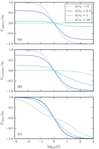
Figure 2: Scaled energies for a point charge at distance $d$ from the surface of a (a) dielectric sphere, (b) cylinder, and (c) slab. The dielectric contrast $\tilde{\kappa}=\kappa_{\mathrm{obj}}/\kappa_{\mathrm{bg}}$ controls the magnitude of dielectric effects. There are three different limiting behaviors when $d\rightarrow\infty$: (a) $U_{\mathrm{sphere}}/u_{0}$ goes to zero, (b) $U_{\mathrm{cylinder}}/u_{0}$ goes to zero except when $\ln\tilde{\kappa}\rightarrow+\infty$, where it goes to $-1$, (c) $U_{\mathrm{slab}}/u_{0}$ goes to $\mp 1$ when $\ln\tilde{\kappa}\rightarrow\pm\infty$.

In Fig. 2 the scaled energies are plotted as functions of $\log_{10}\tilde{\kappa}$. When $d\ll r_{0}$, we recover the asymptotic behavior in Eq. (141). However, when $d\gg r_{0}$, the sphere, cylinder, and slab geometries differ markedly. The sphere energy decays like $d^{-4}$ when $d\gg r_{0}$, and $U_{\mathrm{sphere}}/u_{0}$ goes to $0$ even when $\ln\tilde{\kappa}\rightarrow\pm\infty$. The cylinder energy exhibits a pronounced asymmetry: $U_{\mathrm{cylinder}}/u_{0}$ goes to $0$ when $d\gg r_{0}$, except when $\ln\tilde{\kappa}\rightarrow+\infty$, where $U_{\mathrm{cylinder}}/u_{0}$ goes to $-1$. The slab energy is antisymmetric in dielectric contrast, $U_{\mathrm{slab}}(\tilde{\kappa})=-U_{\mathrm{slab}}(1/\tilde{\kappa})$. It also responds most strongly, with a scaled energy $U_{\mathrm{slab}}/u_{0}$ that goes to $\mp 1$ in both conducting limits $\ln\tilde{\kappa}\rightarrow\pm\infty$, independent of $d$.

The above energy scaling has an interesting connection to the spectrum of $\mathcal{A}$. In Appendix B we solved the exact spectrum of $\mathcal{A}$ for sphere, cylinder, and slab geometries, and found that the ratio of extremal eigenvalues $\lambda_{\mathrm{ratio}}$ is large precisely when the dielectric interaction $U/u_{0}$ is abnormally large: the cylinder when $\ln\tilde{\kappa}\rightarrow\infty$ and the slab when $\ln\tilde{\kappa}\rightarrow\pm\infty$.

References

- Perutz (1978) M. Perutz, Science 201, 1187 (1978).
- Honig and Nicholls (1995) B. Honig and A. Nicholls, Science 268, 1144 (1995).
- Clapham (2007) D. E. Clapham, Cell 131, 1047 (2007).
- Hunter (2001) R. J. Hunter, Foundations of Colloid Science, 2nd ed. (Oxford University Press, Oxford, 2001).
- Leunissen et al. (2005) M. E. Leunissen, C. G. Christova, A.-P. Hynninen, C. P. Royall, A. I. Campbell, A. Imhof, M. Dijkstra, R. van Roij, and A. van Blaaderen, Nature 437, 235 (2005).
- Levin (2005) Y. Levin, Physica A 352, 43 (2005).
- Vernizzi and Olvera de la Cruz (2007) G. Vernizzi and M. Olvera de la Cruz, Proc. Natl. Acad. Sci. U.S.A. 104, 18382 (2007).
- Barros and Luijten (2013) K. Barros and E. Luijten, “Dielectric effects in the self-assembly of binary colloidal aggregates,” (2013), submitted.
- Pohl (1951) H. A. Pohl, J. Appl. Phys. 22, 869 (1951).
- Pohl (1958) H. A. Pohl, J. Appl. Phys. 29, 1182 (1958).
- Jones (1995) T. B. Jones, Electromechanics of particles (Cambridge University Press, Cambridge, U.K., 1995).
- Love (1975) J. D. Love, Quart. J. Mech. Appl. Math. 28, 449 (1975).
- Doerr and Yu (2004) T. P. Doerr and Y.-K. Yu, Am. J. Phys. 72, 190 (2004).
- Doerr and Yu (2006) T. P. Doerr and Y.-K. Yu, Phys. Rev. E 73, 061902 (2006).
- Messina (2002) R. Messina, J. Chem. Phys. 117, 11062 (2002).
- Wynveen and Bresme (2006) A. Wynveen and F. Bresme, J. Chem. Phys. 124, 104502 (2006).
- Maggs and Everaers (2006) A. C. Maggs and R. Everaers, Phys. Rev. Lett. 96, 230603 (2006).
- Rottler and Krayenhoff (2009) J. Rottler and B. Krayenhoff, J. Phys.: Condens. Matter 21, 255901 (2009).
- Marchi et al. (2001) M. Marchi, D. Borgis, N. Levy, and P. Ballone, J. Chem. Phys. 114, 4377 (2001).
- Levy et al. (2005) N. Levy, D. Borgis, and M. Marchi, Comp. Phys. Comm. 169, 69 (2005).
- Levitt (1978) D. G. Levitt, Biophys. J. 22, 209 (1978).
- Zauhar and Morgan (1985) R. Zauhar and R. Morgan, J. Mol. Biol. 186, 815 (1985).
- Hoshi et al. (1987) H. Hoshi, M. Sakurai, Y. Inoue, and R. Chûjô, J. Chem. Phys. 87, 1107 (1987).
- Allen et al. (2001) R. Allen, J.-P. Hansen, and S. Melchionna, Phys. Chem. Chem. Phys. 3, 4177 (2001).
- Boda et al. (2004) D. Boda, D. Gillespie, W. Nonner, D. Henderson, and B. Eisenberg, Phys. Rev. E 69, 046702 (2004).
- Jadhao et al. (2012) V. Jadhao, F. J. Solis, and M. Olvera de la Cruz, Phys. Rev. Lett. 109, 223905 (2012).
- Saad and Schultz (1986) Y. Saad and M. H. Schultz, SIAM J. Sci. Stat. Comput. 7, 856 (1986).
- Bharadwaj et al. (1995) R. Bharadwaj, A. Windemuth, S. Sridharan, B. Honig, and A. Nicholls, J. Comput. Chem. 16, 898 (1995).
- Tyagi et al. (2010) S. Tyagi, M. Süzen, M. Sega, M. Barbosa, S. S. Kantorovich, and C. Holm, J. Chem. Phys. 132, 154112 (2010).
- Karttunen et al. (2008) M. Karttunen, J. Rottler, I. Vattulainen, and C. Sagui, Curr. Top. Membr. 60, 49 (2008).
- Greengard and Rokhlin (1987) L. Greengard and V. Rokhlin, J. Comp. Phys. 73, 325 (1987).
- Greengard and Rokhlin (1997) L. Greengard and V. Rokhlin, Acta Numerica 6, 229 (1997).
- Sagui and Darden (2001) C. Sagui and T. Darden, J. Chem. Phys. 114, 6578 (2001).
- Liang and Subramaniam (1997) J. Liang and S. Subramaniam, Biophys. J. 73, 1830 (1997).
- Landau et al. (1993) L. D. Landau, E. M. Lifshitz, and L. P. Pitaevskii, Electrodynamics of Continuous Media, 2nd ed., Course of Theoretical Physics, Vol. 8 (Elsevier Butterworth Heinemann, Oxford, 1993).
- Marcus (1956) R. A. Marcus, J. Chem. Phys. 24, 966 (1956).
- Felderhof (1977) B. U. Felderhof, J. Chem. Phys. 67, 493 (1977).
- (38) D. Sinkovits, K. Barros, and E. Luijten, in preparation.
- Hoyles et al. (1998) M. Hoyles, S. Kuyucak, and S.-H. Chung, Comp. Phys. Comm. 115, 45 (1998).
- Boda et al. (2005) D. Boda, D. Gillespie, B. Eisenberg, W. Nonner, and D. Henderson, in Ionic Soft Matter: Modern Trends in Theory and Applications, Nato Science Series II: Mathematics, Physics and Chemistry, Vol. 206, edited by D. Henderson, M. Holovko, and A. Trokhymchuk (Springer, Dordrecht, The Netherlands, 2005) pp. 19–43.
- Tausch et al. (2001) J. Tausch, J. Wang, and J. White, IEEE Trans. Comput.-Aided Des. 20, 1398 (2001).
- Bardhan et al. (2009) J. P. Bardhan, R. S. Eisenberg, and D. Gillespie, Phys. Rev. E 80, 011906 (2009).
- Hockney and Eastwood (1981) R. W. Hockney and J. W. Eastwood, Computer Simulation Using Particles (McGraw-Hill, New York, 1981).
- Pollock and Glosli (1996) E. Pollock and J. Glosli, Comp. Phys. Comm. 95, 93 (1996).
- Essmann et al. (1995) U. Essmann, L. Perera, M. L. Berkowitz, T. Darden, H. Lee, and L. G. Pedersen, J. Chem. Phys. 103, 8577 (1995).
- Plimpton (1995) S. J. Plimpton, J. Comp. Phys. 117, 1 (1995).
- Jackson (1999) J. D. Jackson, Classical Electrodynamics, 3rd ed. (Wiley, New York, 1999).
- Richardson (1910) L. F. Richardson, Phil. Trans. Roy. Soc. London A 210, 307 (1910).
- Young (1989) D. M. Young, Comp. Phys. Comm. 53, 1 (1989).
- Saad (2003) Y. Saad, Iterative Methods for Sparse Linear Systems, 2nd ed. (SIAM, Philadelphia, 2003).
- Car and Parrinello (1985) R. Car and M. Parrinello, Phys. Rev. Lett. 55, 2471 (1985).
- Schwinger et al. (1998) J. Schwinger, L. L. Deraad, Jr., K. A. Milton, and W.-y. Tsai, Classical Electrodynamics (Westview Press, Boulder, Colorado, 1998).
- Zangwill (2013) A. Zangwill, Modern Electrodynamics (Cambridge University Press, Cambridge, U.K., 2013).
- Iversen et al. (1998) G. Iversen, Y. I. Kharkats, and J. Ulstrup, Mol. Phys. 94, 297 (1998).
- Cui (2006) S. T. Cui, Mol. Phys. 104, 2993 (2006).