Spectral parameter power series for polynomial pencils of Sturm-Liouville operators and Zakharov-Shabat systems

Abstract.

A spectral parameter power series (SPPS) representation for solutions of Sturm-Liouville equations of the form

$(\ast )$ $$\left(pu^{\prime}\right)^{\prime}+qu=u\sum_{k=1}^{N}\lambda^{k}r_{k}$$

is obtained. It allows one to write a general solution of the equation as a power series in terms of the spectral parameter $\lambda$. The coefficients of the series are given in terms of recursive integrals involving a particular solution of the equation $\left(pu_{0}^{\prime}\right)^{\prime}+qu_{0}=0$. The convenient form of the solution of ($\ast$) provides an efficient numerical method for solving corresponding initial value, boundary value and spectral problems.

A special case of the Sturm-Liouville equation ($\ast$) arises in relation with the Zakharov-Shabat system. We derive an SPPS representation for its general solution and consider other applications as the one-dimensional Dirac system and the equation describing a damped string. Several numerical examples illustrate the efficiency and the accuracy of the numerical method based on the SPPS representations which besides its natural advantages like the simplicity in implementation and accuracy is applicable to the problems admitting complex coefficients, spectral parameter dependent boundary conditions and complex spectrum.

1. Introduction

Equations of the form

(1.1) $$\left(pu^{\prime}\right)^{\prime}+qu=u\sum_{k=1}^{N}\lambda^{k}r_{k}$$

arise in numerous applications and have been studied in a considerable number of publications where sometimes they were referred to as Schrödinger-type equations with a polynomial energy-dependent potential [42, 44], Schrödinger equations with an energy-dependent potential [40], Schrödinger operators with energy depending potentials [38], Klein-Gordon s-wave equations [5], energy-dependent Sturm–Liouville equations [46], pencil of Sturm-Liouville operators [4, 51], polynomial pencil of Sturm-Liouville equations [2] or bundle for Sturm-Liouville operators [43]. Here $p$, $q$ and $r_{k}$, $k=1,\ldots,N$ are complex-valued functions of the real variable $x$ and the complex number $\lambda$ is the spectral parameter. Additional conditions on the coefficients of equation (1.1) will be formulated below.

In the present work we obtain a spectral parameter power series (SPPS) representation for solutions of (1.1). This result generalizes what was done for the Sturm-Liouville equation

(1.2) $$\left(pu^{\prime}\right)^{\prime}+qu=\lambda ru$$

in [31] (see also [32, 33]).

The general solution of (1.1) is represented in the form of a power series in terms of the spectral parameter $\lambda$. The coefficients of the series are calculated as recursive integrals in terms of a particular solution of the equation

(1.3) $$\left(pu_{0}^{\prime}\right)^{\prime}+qu_{0}=0.$$

Moreover, to construct the particular solution one can use the same SPPS approach as was explained in [32, 33].

As was shown in a number of recent publications the SPPS representation provides an efficient and accurate method for solving initial value, boundary value and spectral problems (see [7], [8], [16], [21], [23], [22], [24], [25], [31], [32], [33], [35], [47]). In this paper we demonstrate this fact in application to equation (1.1). The main advantage of the SPPS approach applied to spectral problems consists in the possibility to write down a characteristic (or dispersion) equation of a problem in an explicit form $\Phi(\lambda)=0$ where the function $\Phi$ is analytic with respect to $\lambda$. Due to the SPPS representation the function $\Phi$ is given in the form of a Taylor series whose coefficients can be computed in terms of the particular solution of (1.3). For a numerical computation a partial sum of the Taylor series $\Phi_{M}$ is calculated and the approximate solution of the spectral problem reduces to the problem of finding zeros of the polynomial $\Phi_{M}(\lambda)$. The accuracy of this approach depends on the smallness of the difference $\left|\Phi-\Phi_{M}\right|$ for which we present estimates and additionally show that due to Rouche’s theorem a good approximation of $\Phi$ by $\Phi_{M}$ in a domain $\Omega\subset\mathbb{C}$ guarantees that no root of $\Phi_{M}$ which would correspond to a fictitious eigenvalue can appear in $\Omega$ as a result of truncation of the spectral parameter power series. That is, in a domain $\Omega$ where $\max\left|\Phi-\Phi_{M}\right|$ is sufficiently small all roots of $\Phi_{M}$ approximate true eigenvalues of the spectral problem. We show that for localizing the eigenvalues and for estimating their number in a complex domain the argument principle can be used.

The Zakharov-Shabat system is one of the physical models which can be reduced to an equation of the form (1.1). When the potential in the Zakharov-Shabat system is real valued the situation is simpler in the sense that the system reduces to an equation (1.2) and in that case the SPPS representations were obtained and used for solving spectral problems in [35]. Nevertheless when the potential is complex valued such reduction in general is impossible and an equation of the form (1.1) with $N=2$ naturally arises. We derive an SPPS representation for solutions of such general Zakharov-Shabat system as well as an analytic form for the dispersion equation of the corresponding spectral problem in the case of a compactly supported potential. The numerical implementation of the method together with the argument principle is illustrated on a couple of test problems. We show that the one-dimensional Dirac system can be studied in a similar way.

Another physical model considered in this paper and reducing to an equation of the form (1.1) again with $N=2$ corresponds to a damped string [3, 19, 29]. We obtain an analytic form for the dispersion equation of the corresponding spectral problem and illustrate the application of the SPPS method on a number of numerical examples.

2. SPPS representation for solutions of (1.1)

In this section we derive and prove an SPPS representation for the general solution of (1.1).

Theorem 2.1.

Suppose that on a finite segment $\left[a,b\right]$ the equation

$$\left(pv^{\prime}\right)^{\prime}+qv=0$$

possesses a particular non-vanishing solution $u_{0}$ such that the functions $u_{0}^{2}r_{k}$, $k=1,\ldots,N$ and $\frac{1}{u_{0}^{2}p}$ are continuous on $\left[a,b\right]$. Then a general solution of the equation

(2.1) $$\left(pu^{\prime}\right)^{\prime}+qu=u\sum_{k=1}^{N}\lambda^{k}r_{k}$$

has the form $u=c_{1}u_{1}+c_{2}u_{2}$, where $c_{1}$ and $c_{2}$ are arbitrary complex constants,

(2.2) $$u_{1}=u_{0}\sum_{n=0}^{\infty}\lambda^{n}\widetilde{X}^{\left(2n\right)}\quad\text{ and }\quad u_{2}=u_{0}\sum_{n=0}^{\infty}\lambda^{n}X^{\left(2n+1\right)}$$

with $\widetilde{X}^{\left(n\right)}$ and $\ X^{\left(n\right)}$ being defined by the recursive relations

$$\widetilde{X}^{\left(n\right)} \equiv X^{\left(n\right)}\equiv 0\quad\text{ for }n<0,$$

$$\widetilde{X}^{\left(0\right)} \equiv X^{\left(0\right)}\equiv 1,$$

and

(2.3) $$\widetilde{X}^{\left(n\right)}\left(x\right) =\begin{cases}\intop_{x_{0}}^{x}u_{0}^{2}\left(y\right)\sum_{k=1}^{N}\widetilde{X}^{\left(n-2k+1\right)}\left(y\right)r_{k}\left(y\right)dy&n\text{-odd}\\ \intop_{x_{0}}^{x}\widetilde{X}^{\left(n-1\right)}\left(y\right)\frac{1}{u_{0}^{2}\left(y\right)p\left(y\right)}dy&n\text{-even,}\end{cases}$$

(2.4) $$X^{\left(n\right)}\left(x\right) =\begin{cases}\intop_{x_{0}}^{x}X^{\left(n-1\right)}\left(y\right)\frac{1}{u_{0}^{2}\left(y\right)p\left(y\right)}dy&n\text{-odd}\\ \intop_{x_{0}}^{x}u_{0}^{2}\left(y\right)\sum_{k=1}^{N}X^{\left(n-2k+1\right)}\left(y\right)r_{k}\left(y\right)dy&n\text{-even,}\end{cases}$$

where $x_{0}$ is an arbitrary point of $\left[a,b\right]$ such that $p(x_{0})\neq 0$. Both series in (2.2) converge uniformly on $\left[a,b\right]$.

Proof.

We prove first that $u_{1}$ and $u_{2}$ are indeed solutions of (2.1) whenever the application of the operator $L=\frac{d}{dx}p\frac{d}{dx}+q$ makes sense. If $u_{0}$ is a non-vanishing solution of $Lu_{0}=0$, then the operator $L=\frac{d}{dx}p\frac{d}{dx}+q$ admits the Pólya factorization $L=\frac{1}{u_{0}}\partial pu_{0}^{2}\partial\frac{1}{u_{0}}$. Application of $L$ to $u_{1}$ using (2.3) gives

$$Lu_{1} =\frac{1}{u_{0}}\partial pu_{0}^{2}\partial\sum_{k=0}^{\infty}\lambda^{k}\widetilde{X}^{\left(2k\right)}=\frac{1}{u_{0}}\sum_{k=1}^{\infty}\lambda^{k}\partial\widetilde{X}^{\left(2k-1\right)}$$

$$=\frac{1}{u_{0}}\sum_{k=1}^{\infty}\lambda^{k}\sum_{n=1}^{N}\widetilde{X}^{\left(2\left(k-n\right)\right)}u_{0}^{2}r_{n}=\sum_{n=1}^{N}r_{n}u_{0}\sum_{k=1}^{\infty}\lambda^{k}\widetilde{X}^{\left(2\left(k-n\right)\right)}$$

$$=\sum_{n=1}^{N}r_{n}u_{0}\sum_{k=n}^{\infty}\lambda^{k}\widetilde{X}^{\left(2\left(k-n\right)\right)}=\sum_{n=1}^{N}r_{n}u_{0}\sum_{k=0}^{\infty}\lambda^{k+n}\widetilde{X}^{\left(2k\right)}$$

$$=\sum_{n=1}^{N}r_{n}\lambda^{n}u_{0}\sum_{k=0}^{\infty}\lambda^{k}\widetilde{X}^{\left(2k\right)}=u_{1}\sum_{n=1}^{N}\lambda^{n}r_{n}.$$

Similarly, application of $L$ to $u_{2}$ shows that $u_{2}$ satisfies (2.1).

In order to give sense to this chain of equalities it is sufficient to prove the uniform convergence of the series involved in $u_{1}$ and $u_{2}$ as well as the uniform convergence of the series obtained by a term-wise differentiation of $\frac{u_{1}}{u_{0}}$ and $\frac{u_{2}}{u_{0}}$. First, we prove the uniform convergence of the series involved in $u_{1}$. This can be done with the aid of the Weierstrass M-test.

We prove by induction that for $n\geq 0$ the inequality

(2.5) $$\left|\widetilde{X}^{\left(2n\right)}(x)\right|\leq\sum_{k=0}^{n-\left[\frac{n}{N}\right]}\binom{n}{k}\frac{\left(m\left|x-x_{0}\right|\right)^{2\left(n-k\right)}}{\left(2\left(n-k\right)\right)!}$$

is valid, where $m$ denotes the maximum of the functions $\left|u_{0}^{2}(x)r_{k}(x)\right|$, $k=1,\ldots,N$ and $\bigl{|}\frac{1}{u_{0}^{2}\left(x\right)p\left(x\right)}\bigr{|}$ on $[a,b]$. For $n=0$, $|\widetilde{X}^{\left(0\right)}|=1$, and hence (2.5) holds. For the inductive step we assume that (2.5) holds for some $n$ and prove that for $n+1$ the inequality

(2.6) $$\left|\widetilde{X}^{\left(2\left(n+1\right)\right)}(x)\right|\leq\sum_{k=0}^{n+1-\left[\frac{n+1}{N}\right]}\binom{n+1}{k}\frac{\left(m\left|x-x_{0}\right|\right)^{2\left(n+1-k\right)}}{\left(2\left(n+1-k\right)\right)!}$$

holds. Suppose that $x_{0}\leq x$ (the opposite case is similar), recalling the definition of $m$ and (2.3) we have

$$\left|\widetilde{X}^{\left(2\left(n+1\right)\right)}(x)\right| =\left|\intop_{x_{0}}^{x}\widetilde{X}^{\left(2n+1\right)}\left(y\right)\frac{1}{u_{0}^{2}\left(y\right)p\left(y\right)}dy\right|\leq m\intop_{x_{0}}^{x}\left|\widetilde{X}^{\left(2n+1\right)}\left(y\right)\right|dy$$

$$\leq m\intop_{x_{0}}^{x}\intop_{x_{0}}^{y}\sum_{j=1}^{N}\left|\widetilde{X}^{\left(2\left(n-j+1\right)\right)}\left(z\right)u_{0}^{2}\left(z\right)r_{j}\left(z\right)\right|dzdy$$

$$\leq m^{2}\intop_{x_{0}}^{x}\intop_{x_{0}}^{y}\sum_{j=1}^{N}\left|\widetilde{X}^{\left(2\left(n-j+1\right)\right)}\left(z\right)\right|dzdy=m^{2}\intop_{x_{0}}^{x}\intop_{x_{0}}^{y}\sum_{j=1}^{\min\{n+1,N\}}\left|\widetilde{X}^{\left(2\left(n-j+1\right)\right)}\left(z\right)\right|dzdy.$$

Applying (2.5) one obtains

$$\left|\widetilde{X}^{\left(2\left(n+1\right)\right)}(x)\right| \leq m^{2}\intop_{x_{0}}^{x}\intop_{x_{0}}^{y}\sum_{j=1}^{\min\{n+1,N\}}\sum_{k=0}^{n-j+1-\left[\frac{n-j+1}{N}\right]}\binom{n-j+1}{k}\frac{\left(m\left|z-x_{0}\right|\right)^{2\left(n-j-k+1\right)}}{\left(2\left(n-j-k+1\right)\right)!}dzdy$$

$$=\sum_{j=1}^{\min\{n+1,N\}}\sum_{k=0}^{n-j+1-\left[\frac{n-j+1}{N}\right]}\frac{\binom{n-j+1}{k}m^{2\left(n-j-k+2\right)}}{\left(2\left(n-j-k+1\right)\right)!}\intop_{x_{0}}^{x}\intop_{x_{0}}^{y}\left|z-x_{0}\right|^{2\left(n-j-k+1\right)}dzdy$$

$$=\sum_{j=1}^{\min\{n+1,N\}}\sum_{k=0}^{n-j+1-\left[\frac{n-j+1}{N}\right]}\binom{n-j+1}{k}\frac{\left(m\left|x-x_{0}\right|\right)^{2\left(n-j-k+2\right)}}{\left(2\left(n-j-k+2\right)\right)!}.$$

It is easy to see that from $1\leq j\leq\min\{n+1,N\}$ and $0\leq k\leq n-j+1-\left[\frac{n-j+1}{N}\right]$ it follows that

$$0\leq k+j-1\leq n+1-\left[\frac{n+1}{N}\right].$$

We rearrange the terms with respect to $l=k+j-1$,

$$\sum_{j=1}^{\min\{n+1,N\}}\sum_{k=0}^{n-j+1-\left[\frac{n-j+1}{N}\right]}\binom{n-j+1}{k}\frac{\left(m\left|x-x_{0}\right|\right)^{2\left(n-j-k+2\right)}}{\left(2\left(n-j-k+2\right)\right)!}$$

$$\qquad=\sum_{l=0}^{n+1-\left[\frac{n+1}{N}\right]}\sum_{j=1}^{\min\{N,n+1,l+1\}}\binom{n-(j-1)}{l-(j-1)}\frac{\left(m\left|x-x_{0}\right|\right)^{2\left(n+1-l\right)}}{\left(2\left(n+1-l\right)\right)!}$$

$$\qquad\leq\sum_{l=0}^{n+1-\left[\frac{n+1}{N}\right]}\frac{\left(m\left|x-x_{0}\right|\right)^{2\left(n+1-l\right)}}{\left(2\left(n+1-l\right)\right)!}\sum_{j=0}^{l}\binom{n-j}{l-j}.$$

Using the well known combinatorial relation

$$\binom{n+1}{l}=\sum_{j=0}^{l}\binom{n-j}{l-j}\qquad\text{ for }l<n+1$$

we obtain

$$\sum_{l=0}^{n+1-\left[\frac{n+1}{N}\right]}\frac{\left(m\left|x-x_{0}\right|\right)^{2\left(n+1-l\right)}}{\left(2\left(n+1-l\right)\right)!}\sum_{j=0}^{l}\binom{n-j}{l-j}=\sum_{l=0}^{n+1-\left[\frac{n+1}{N}\right]}\frac{\left(m\left|x-x_{0}\right|\right)^{2\left(n+1-l\right)}}{\left(2\left(n+1-l\right)\right)!}\binom{n+1}{l},$$

which finishes the proof of (2.6) and hence of the estimate (2.5) for any integer $n\geq 0$.

Next we prove that the series $\sum_{n=0}^{\infty}\lambda^{n}\widetilde{X}^{\left(2n\right)}$ converges uniformly on $\left[a,b\right]$. We have for $n\geq 0$

$$\left|\widetilde{X}^{\left(2n\right)}(x)\right| \leq\sum_{k=0}^{n-\left[\frac{n}{N}\right]}\binom{n}{k}\frac{\left(m\left|x-x_{0}\right|\right)^{2\left(n-k\right)}}{\left(2\left(n-k\right)\right)!}\leq\sum_{k=0}^{n-\left[\frac{n}{N}\right]}\binom{n}{k}\frac{\left(m\left(b-a\right)\right)^{2\left(n-k\right)}}{\left(2\left[\frac{n}{N}\right]\right)!}$$

$$\leq\frac{1}{\left(2\left[\frac{n}{N}\right]\right)!}\sum_{k=0}^{n}\binom{n}{k}\left(m\left(b-a\right)\right)^{2\left(n-k\right)}1^{k}=\frac{\left(\left(m\left(b-a\right)\right)^{2}+1\right)^{n}}{\left(2\left[\frac{n}{N}\right]\right)!}.$$

Hence

$$\sum_{n=0}^{\infty}\left|\lambda\right|^{n}\left|\widetilde{X}^{\left(2n\right)}\right|\leq\sum_{n=0}^{\infty}\left|\lambda\right|^{n}\frac{\left(\left(m\left(b-a\right)\right)^{2}+1\right)^{n}}{\left(2\left[\frac{n}{N}\right]\right)!},$$

and grouping terms with respect to $n_{1}=[\frac{n}{N}]$ we obtain

$$\sum_{n=0}^{\infty}\left|\lambda\right|^{n}\left|\widetilde{X}^{\left(2n\right)}\right|\leq\sum_{n_{1}=0}^{\infty}\left|\lambda\right|^{n_{1}N}\frac{\left(\left(m\left(b-a\right)\right)^{2}+1\right)^{n_{1}N}}{\left(2n_{1}\right)!}\sum_{k=0}^{N-1}\left|\lambda\right|^{k}\left(\left(m\left(b-a\right)\right)^{2}+1\right)^{k}.$$

Considering the notation $M=\left|\lambda\right|\left(\left(m\left(b-a\right)\right)^{2}+1\right)$ one obtains

$$\sum_{n=0}^{\infty}\left|\lambda\right|^{n}\left|\widetilde{X}^{\left(2n\right)}\right|\leq\sum_{k=0}^{N-1}M^{k}\sum_{n_{1}=0}^{\infty}\frac{M^{n_{1}N}}{(2n_{1})!}=\sum_{k=0}^{N-1}M^{k}\cosh M^{N/2}.$$

Then, by the Weierstrass M-test the series $\sum_{n=0}^{\infty}\lambda^{n}\widetilde{X}^{\left(2n\right)}$ converges uniformly on $\left[a,b\right]$.

The proof for the function $u_{2}$ and the derivatives $\left(\frac{u_{1}}{u_{0}}\right)^{\prime}=\frac{1}{u_{0}p}\sum_{n=0}^{\infty}\lambda^{n+1}\widetilde{X}^{(2n+1)}$ and $\left(\frac{u_{2}}{u_{0}}\right)^{\prime}=\frac{1}{u_{0}p}\sum_{n=0}^{\infty}\lambda^{n}X^{(2n)}$ is similar. The last step is to verify that the Wronskian of $u_{1}$ and $u_{2}$ is different from zero at least at one point (which necessarily implies the linear independence of $u_{1}$ and $u_{2}$ on the whole segment $[a,b]$). It is easy to see that by definition all $\widetilde{X}^{(n)}(x_{0})$ and $X^{(n)}(x_{0})$ vanish except $\widetilde{X}^{(0)}(x_{0})=X^{(0)}(x_{0})=1$. Thus

(2.7) $$u_{1}\left(x_{0}\right) =u_{0}\left(x_{0}\right), u_{1}^{\prime}\left(x_{0}\right) =u_{0}^{\prime}\left(x_{0}\right),$$

(2.8) $$u_{2}\left(x_{0}\right) =0, u_{2}^{\prime}\left(x_{0}\right) =\frac{1}{u_{0}\left(x_{0}\right)p\left(x_{0}\right)},$$

and hence the Wronskian of $u_{1}$ and $u_{2}$ at $x_{0}$ is $\frac{1}{p\left(x_{0}\right)}\neq 0$. ∎

Remark 2.2.

The particular solution $u_{0}$ which in general can be complex valued may be constructed by means of the SPPS representation as well (see [32, 33]).

When $N=1$, the result of Theorem 2.1 reduces to the SPPS representation for solutions of a classic Sturm-Liouville equation presented in [33].

Example 2.3.

Consider the differential equation

$$y^{\prime\prime}=y(\lambda+2\lambda^{2})$$

on the segment $\left[0,1\right]$ with the initial conditions

(2.9) $$y\left(0\right)=1\quad\text{and}\quad y^{\prime}\left(0\right)=0.$$

The unique solution of this problem has the form $y(x)=\cosh\left(x\sqrt{\lambda+2\lambda^{2}}\right)$. This is an equation of the form (2.1) with $p=1$, $q=0$ and $r_{k}=k$, $k=1,2$. Let us consider its solution in terms of the SPPS representation from Theorem 2.1. Taking $x_{0}=0$ and $u_{0}\equiv 1$ as a particular solution of the differential equation $y^{\prime\prime}=0$ we compute the functions $\widetilde{X}^{\left(2n\right)}$ for $n=1,2,3$ to find the first terms of the series $u_{1}=u_{0}\sum_{k=0}^{\infty}\lambda^{k}\widetilde{X}^{\left(2k\right)}$,

$$\begin{array}[]{cc}n&\widetilde{X}^{\left(2n\right)}\\ 1&\frac{x^{2}}{2}\\ 2&x^{2}+\frac{x^{4}}{24}\\ 3&\frac{x^{4}}{6}+\frac{x^{6}}{720}\\ \vdots&\vdots\end{array}$$

Thus, the first four terms of the SPPS representation of $u_{1}$ have the form

(2.10) $$u_{1}(x)=1+\frac{x^{2}}{2}\lambda+\left(x^{2}+\frac{x^{4}}{24}\right)\lambda^{2}+\left(\frac{x^{4}}{6}+\frac{x^{6}}{720}\right)\lambda^{3}+\cdots.$$

Notice that due to (2.7) the solution $u_{1}$ satisfies (2.9) and hence must coincide with $y$. Indeed, computation of the first four terms of the Taylor series of the exact solution $y$ with respect to the spectral parameter $\lambda$ gives us again (2.10).

3. Spectral shift technique

The procedure for constructing solutions of equation (2.1) described in Theorem 2.1 works when a particular solution is available for $\lambda=0$ (analytically or numerically). In [33] it was mentioned that for equation (1.2) it is also possible to construct the SPPS representation of a general solution starting from a non-vanishing particular solution for some $\lambda=\lambda_{0}$. Such procedure is called spectral shift and has already proven its usefulness for numerical applications [9, 21, 33].

We show that a spectral shift technique may also be applied to equation (2.1). Let $\lambda_{0}$ be a fixed complex number (not necessarily an eigenvalue). Suppose that on the finite interval $\left[a,b\right]$ a non-vanishing solution $u_{0}$ of the equation

(3.1) $$(pu_{0}^{\prime})^{\prime}+qu_{0}=u_{0}\sum_{k=1}^{N}\lambda_{0}^{k}r_{k}$$

is known, such that the functions $u_{0}^{2}r_{k}$, $k=1,\ldots,N$ and $\frac{1}{u_{0}^{2}p}$ are continuous on $\left[a,b\right]$. Let $\lambda=\lambda_{0}+\Lambda$ then the right hand side of (2.1) can be written in the form

$$u\sum_{k=1}^{N}\left(\lambda_{0}+\Lambda\right)^{k}r_{k} =u\sum_{k=1}^{N}r_{k}\sum_{\ell=0}^{k}\binom{k}{\ell}\lambda_{0}^{\ell}\Lambda^{k-\ell}$$

$$=u\sum_{k=1}^{N}r_{k}\lambda_{0}^{k}+u\sum_{k=1}^{N}\Lambda^{k}\sum_{\ell=0}^{N-k}\binom{k+\ell}{\ell}\lambda_{0}^{\ell}r_{k+\ell}.$$

Due to this identity equation (2.1) is transformed again into an equation of the form (2.1):

(3.2) $$L_{0}u=u\sum_{k=1}^{N}\Lambda^{k}\sum_{\ell=0}^{N-k}\binom{k+\ell}{\ell}\lambda_{0}^{\ell}r_{k+\ell},$$

where

$$L_{0}u=(pu^{\prime})^{\prime}+u\left(q-\sum_{k=1}^{N}r_{k}\lambda_{0}^{k}\right).$$

Now the procedure described in Theorem 2.1 can be applied to equation (3.2). Considering the particular solution $u_{0}$ of (3.1) and the functions

$$\tilde{r}_{k}=\sum_{\ell=0}^{N-k}\binom{k+\ell}{\ell}\lambda_{0}^{\ell}r_{k+\ell}$$

one can construct the system of recursive integrals $X^{(n)}$ and $\widetilde{X}^{(n)}$ by applying (2.3) and (2.4) to functions $u_{0}$ and $\tilde{r}_{k}$. Then the general solution of equation (2.1) has the form $u=c_{1}u_{1}+c_{2}u_{2}$ where $c_{1}$ and $c_{2}$ are arbitrary complex constants and

$$u_{1}=u_{0}\sum_{n=0}^{\infty}\left(\lambda-\lambda_{0}\right)^{n}\widetilde{X}^{\left(2n\right)}\quad\text{and}\quad u_{2}=u_{0}\sum_{n=0}^{\infty}\left(\lambda-\lambda_{0}\right)^{n}X^{\left(2n+1\right)}.$$

4. The generalized Zakharov-Shabat system

The Zakharov-Shabat system arises in the Inverse Scattering Transform method when integrating the non-linear Schrödinger equation, see, e.g., [1, 15, 18, 23, 35, 50, 52, 54]. In the recent work [35] an SPPS representation was obtained for the solutions of the Zakharov-Shabat system with a real-valued potential. In this section we consider the generalized Zakharov-Shabat system, also sometimes called the one-dimensional Dirac system [23]

(4.1) $$v_{1}^{\prime} =\lambda v_{1}+Pv_{2}$$

(4.2) $$v_{2}^{\prime} =-\lambda v_{2}-Qv_{1},$$

where $v_{1}$ and $v_{2}$ are unknown complex valued functions of the independent variable $x$, $\lambda\in\mathbb{C}$ is a constant, $Q$ and $P$ are complex-valued functions such that $Q$ does not vanish on the domain of interest.

From (4.2) we have

(4.3) $$v_{1}=-\frac{1}{Q}\left(v_{2}^{\prime}+\lambda v_{2}\right).$$

Substituting this expression into (4.1) we obtain an equation of the form (2.1):

(4.4) $$\left(\frac{1}{Q}v_{2}^{\prime}\right)^{\prime}+Pv_{2}=\lambda\frac{Q^{\prime}}{Q^{2}}v_{2}+\lambda^{2}\frac{1}{Q}v_{2}.$$

4.1. SPPS for the generalized Zakharov-Shabat system

In this subsection, applying the SPPS method to equation (4.4) we obtain an SPPS representation for solutions of the system (4.1), (4.2). The following statement is a direct application of Theorem 2.1 to equation (4.4).

Corollary 4.1.

Suppose that on a finite segment $\left[a,b\right]$ the equation

(4.5) $$\left(\frac{1}{Q}v^{\prime}\right)^{\prime}+Pv=0.$$

possesses a non vanishing particular solution $v_{0}\in C^{1}[a,b]$ such that $\frac{v_{0}^{\prime}}{Q}\in C^{1}[a,b]$ and the functions $v_{0}^{2}\frac{Q^{\prime}}{Q^{2}}$, $\frac{v_{0}^{2}}{Q}$ and $\frac{Q}{v_{0}^{2}}$ are continuous on $\left[a,b\right]$. Then the general solution of (4.4) has the form $v_{2}=c_{1}g_{1}+c_{2}g_{2}$, where $c_{1}$ and $c_{2}$ are arbitrary complex constants,

(4.6) $$g_{1}=v_{0}\sum_{k=0}^{\infty}\lambda^{k}\widetilde{X}^{\left(2k\right)}\quad\text{and}\quad g_{2}=v_{0}\sum_{k=0}^{\infty}\lambda^{k}X^{\left(2k+1\right)}$$

with $\widetilde{X}^{\left(n\right)}$ and $X^{\left(n\right)}$ being defined by the recursive relations

$$\widetilde{X}^{\left(n\right)} \equiv X^{\left(n\right)}\equiv 0\qquad\text{for }n<0,$$

$$\widetilde{X}^{\left(0\right)} \equiv X^{\left(0\right)}\equiv 1,$$

and

(4.7) $$\widetilde{X}^{\left(n\right)}\left(x\right) =\begin{cases}\intop_{x_{0}}^{x}\left(\widetilde{X}^{\left(n-1\right)}\left(y\right)v_{0}^{2}\left(y\right)\frac{Q^{\prime}\left(y\right)}{Q^{2}\left(y\right)}+\widetilde{X}^{\left(n-3\right)}\left(y\right)\frac{v_{0}^{2}\left(y\right)}{Q\left(y\right)}\right)dy,&n\text{-odd}\\ \intop_{x_{0}}^{x}\widetilde{X}^{\left(n-1\right)}\left(y\right)\frac{Q\left(y\right)}{v_{0}^{2}\left(y\right)}dy,&n\text{-even}\end{cases}$$

(4.8) $$X^{\left(n\right)}\left(x\right) =\begin{cases}\intop_{x_{0}}^{x}X^{\left(n-1\right)}\left(y\right)\frac{Q\left(y\right)}{v_{0}^{2}\left(y\right)}dy,&n\text{-odd}\\ \intop_{x_{0}}^{x}\left(X^{\left(n-1\right)}\left(y\right)v_{0}^{2}\left(y\right)\frac{Q^{\prime}\left(y\right)}{Q^{2}\left(y\right)}+X^{\left(n-3\right)}\left(y\right)\frac{v_{0}^{2}\left(y\right)}{Q\left(y\right)}\right)dy,&n\text{-even}\end{cases}$$

where $x_{0}$ is an arbitrary point of $\left[a,b\right]$. Furthermore, both series in (4.6) converge uniformly on $\left[a,b\right]$.

Corollary 4.1 allows us to construct a general solution of the Zakharov-Shabat system.

Theorem 4.2.

Under the conditions of Corollary 4.1 the general solution of the system (4.1), (4.2) has the form

(4.9) $$v_{1} =-c_{1}\left(\frac{v_{0}^{\prime}+\lambda v_{0}}{Q}\sum_{k=0}^{\infty}\lambda^{k}\widetilde{X}^{\left(2k\right)}+\frac{\lambda}{v_{0}}\sum_{k=0}^{\infty}\lambda^{k}\widetilde{X}^{\left(2k+1\right)}\right)$$

$$\qquad-c_{2}\left(\frac{v_{0}^{\prime}+\lambda v_{0}}{Q}\sum_{k=0}^{\infty}\lambda^{k}X^{\left(2k+1\right)}+\frac{1}{v_{0}}\sum_{k=0}^{\infty}\lambda^{k}X^{\left(2k\right)}\right),$$

(4.10) $$v_{2} =c_{1}v_{0}\sum_{k=0}^{\infty}\lambda^{k}\widetilde{X}^{\left(2k\right)}+c_{2}v_{0}\sum_{k=0}^{\infty}\lambda^{k}X^{\left(2k+1\right)}$$

where $c_{1}$ and $c_{2}$ are arbitrary complex constants and the functions $X^{(n)}$ and $\widetilde{X}^{(n)}$ are the same as in Corollary 4.1.

Proof.

By Corollary 4.1 a general solution of (4.4) is given by (4.10). Define $v_{1}$ by (4.3), then $v_{1}$ has the form (4.9) and the pair $v_{1}$, $v_{2}$ satisfy (4.1), (4.2). ∎

Remark 4.3.

In comparison with [35] where the additional conditions $Q=P$ and $Q$ being real-valued were required, this theorem establishes the SPPS representation for solutions of the system (4.1), (4.2) allowing complex-valued coefficients, additionally requiring one of them being non-vanishing.

4.2. The Zakharov-Shabat eigenvalue problem

In this subsection we consider classical Zakharov-Shabat systems characterized by the condition $Q=P^{\ast}$ (where $\ast$ denotes the complex conjugation). This case arises in physical models associated with optical solitons, see, e.g., [1, 15, 26, 27, 35, 54].

Definition 4.4 ([26, 27]).

Solutions of the Zakharov-Shabat system (4.1), (4.2) satisfying the following asymptotic relations:

$$\overrightarrow{\sigma} \cong\binom{1}{0}e^{\lambda x},\qquad x\rightarrow-\infty$$

$$\overrightarrow{\xi} \cong\binom{0}{1}e^{-\lambda x},\qquad x\rightarrow+\infty$$

for some $\lambda$ with $\operatorname{Re}\lambda>0$, are called Jost solutions. Expression $\binom{\sigma_{1}}{\sigma_{2}}\cong\binom{1}{0}e^{\lambda x},$ $x\rightarrow\pm\infty$ means that there exists $\lim_{x\rightarrow\pm\infty}\frac{\sigma_{1}(x)}{e^{\lambda x}}=c$, $c\neq 0$, while $\sigma_{2}(x)=o\left(\sigma_{1}(x)\right)$, $x\rightarrow\pm\infty$.

The eigenvalue problem for the Zakharov-Shabat system consists in finding such values of the spectral parameter $\lambda$ for which there exists a nontrivial Jost solution.

In particular, when the potential $Q$ is compactly supported on $\left[-a,a\right]$ (this situation usually appears after truncating an infinitely supported potential), it is easy to see that the eigenvalue problem reduces to finding such values of $\lambda$ ($\operatorname{Re}\lambda>0$) for which there exists a solution of (4.1), (4.2) on $(-a,a)$ satisfying the following boundary conditions (see, e.g., [27], [28], [35])

(4.11) $$v_{1}\left(-a\right)=1,\quad v_{2}\left(-a\right)=0,$$

(4.12) $$v_{1}\left(a\right) =0.$$

We assume additionally that the potential $Q$ does not vanish on its support.

4.3. Dispersion equation for the eigenvalue problem

In this subsection we write down the dispersion (or characteristic) equation equivalent to the Zakharov-Shabat eigenvalue problem with a compactly supported potential.

Theorem 4.5.

Let $Q$ be a continuous complex-valued non-vanishing function on $\left[-a,a\right]$, and $v_{0}$ be a particular non-vanishing solution of (4.5) satisfying the conditions of Corollary 4.1. Then $\lambda$ ($\operatorname{Re}\lambda>0$) is an eigenvalue of the spectral problem for the Zakharov-Shabat system (4.1), (4.2), (4.11), (4.12) if and only if the following equation is satisfied

(4.13) $$\sum_{k=0}^{\infty}\lambda^{k}\left(v_{0}\left(a\right)\left(v_{0}^{\prime}\left(a\right)X^{\left(2k+1\right)}(a)+v_{0}\left(a\right)X^{\left(2k-1\right)}\left(a\right)\right)+Q(a)X^{\left(2k\right)}\left(a\right)\right)=0,$$

where the functions $X^{(n)}$ are defined by (4.8) with $x_{0}=-a$.

Proof.

Considering $v_{1}$ and $v_{2}$ from Theorem 4.2 with $x_{0}=-a$ we have $v_{1}\left(-a\right)=-c_{1}\left(\frac{v_{0}^{\prime}+\lambda v_{0}\left(-a\right)}{Q\left(-a\right)}\right)-c_{2}\left(\frac{1}{v_{0}\left(-a\right)}\right)$ and $v_{2}\left(-a\right)=c_{1}v_{0}(-a)$. From the boundary condition (4.11) we obtain that $c_{1}=0$ and $c_{2}=-v_{0}\left(-a\right)$. According to the boundary condition (4.12) we obtain that the characteristic equation has the form

$$\frac{v_{0}^{\prime}\left(a\right)+\lambda v_{0}\left(a\right)}{Q\left(a\right)}\sum_{k=0}^{\infty}\lambda^{k}X^{\left(2k+1\right)}\left(a\right)+\frac{1}{v_{0}\left(a\right)}\sum_{k=0}^{\infty}\lambda^{k}X^{\left(2k\right)}\left(a\right)=0$$

which is equivalent to (4.13) taking into account that $X^{(-1)}\equiv 0$. ∎

Remark 4.6.

When $Q$ is real valued, the characteristic equation from [35] can be used since it was obtained without requiring that $Q$ should be non-vanishing.

Remark 4.7.

It is possible to apply the spectral shift technique described in Section 3 to the solution of the Zakharov-Shabat system. Note that we change $\lambda$ by $\lambda-\lambda_{0}$ only in (4.6) and keep the parameter $\lambda$ in (4.3). Hence the characteristic equation (4.13) under the spectral shift becomes

(4.14) $$\sum_{k=0}^{\infty}(\lambda-\lambda_{0})^{k}\left(v_{0}\left(a\right)\left((v_{0}^{\prime}\left(a\right)+\lambda_{0}v_{0}\left(a\right))X^{\left(2k+1\right)}(a)+v_{0}\left(a\right)X^{\left(2k-1\right)}\left(a\right)\right)+Q(a)X^{\left(2k\right)}\left(a\right)\right)=0.$$

This theorem reduces the Zakharov-Shabat eigenvalue problem with a compactly supported potential to the problem of localizing zeros (in the right half-plane) of an analytic function $\Phi(\lambda)=\sum_{k=0}^{\infty}a_{k}\lambda^{k}$ of the complex variable $\lambda$ with the Taylor coefficients $a_{k}$ given by the expressions,

$$a_{k}=v_{0}\left(a\right)\left(v_{0}^{\prime}\left(a\right)X^{\left(2k+1\right)}+v_{0}\left(a\right)X^{\left(2k-1\right)}\left(a\right)\right)+Q(a)X^{\left(2k\right)}\left(a\right).$$

The coefficients $a_{k}$ can be easily and accurately calculated following the definitions introduced above. For the numerical solution of the eigenvalue problem one can truncate the series (4.13) and consider a polynomial

(4.15) $$\Phi_{M}\left(\lambda\right)=\sum_{k=0}^{M}a_{k}\lambda^{k}$$

approximating the function $\Phi$. For a reasonably large $M$ some of its roots give an accurate approximation of the eigenvalues of the problem. The Rouché theorem establishes, see, e.g., [10, Section 3], that if the complex-valued functions $f$ and $g$ are holomorphic inside and on some closed simple contour $K$, with $|g(z)|<|f(z)|$ on $K$, then $f$ and $f+g$ have the same number of zeros inside $K$, where each zero is counted as many times as its multiplicity. As it follows from the Rouché theorem, the roots of $\Phi_{M}$ closest to zero give an accurate approximation of the eigenvalue problem whilst the roots more distant from the origin are spurious roots appearing due to the truncation. Indeed, consider a domain $\Omega$ in the complex plane of the variable $\lambda$ such that

(4.16) $$\min_{\lambda\in\partial\Omega}\left|\Phi_{M}\left(\lambda\right)\right|>\max_{\lambda\in\partial\Omega}\left|\Phi(\lambda)-\Phi_{M}\left(\lambda\right)\right|$$

(that is, $f=\Phi_{M}$, $g=\Phi-\Phi_{M}$ and hence $f+g=\Phi$). Then the number of zeros of $\Phi_{M}$ in $\Omega$ coincides with the number of zeros of $\Phi$, or which is the same with the number of eigenvalues located in $\Omega$. In other words, in a domain $\Omega$ where $\Phi_{M}$ approximates sufficiently closely the function $\Phi$ (the inequality (4.16) should be fulfilled) all the roots of $\Phi_{M}$ approximate the true eigenvalues of the spectral problem. In order to estimate the quantity $\max_{\lambda\in\partial\Omega}\left|\Phi(\lambda)-\Phi_{M}\left(\lambda\right)\right|$ the estimates derived in the proof of Theorem 2.1 can be used. Obviously, the same reasoning is applicable to the characteristic function from (4.14) centered in some $\lambda_{0}$.

The following example illustrates the application of the SPPS method to a Zakharov-Shabat spectral problem admitting complex eigenvalues.

Example 4.8.

Consider the Zakharov-Shabat system with the potential

(4.17) $$Q(x)=\begin{cases}s\left(-1+3\frac{\pi}{4}+3x^{2}\right),&-1\leq x\leq 1,\\ 0,&\text{ otherwise}\end{cases}$$

where $s\in\mathbb{R}$. This potential was considered in a numerical experiment in [27].

According to [27], there is a pair of complex eigenvalues located symmetrically about the real axis in the right half-plane when $s$ is in the range $0.956\leq s\leq 0.9999$. As $s$ increases the eigenvalues $\lambda_{1}$ and $\lambda_{2}$ approach each other and eventually coalesce into a double eigenvalue. If we further increase the parameter $s$ a pair of real eigenvalues appear after the passage through a double eigenvalue state. Table 1 computed by means of the SPPS method illustrates the described phenomenon. With the help of the SPPS representation we found more precisely the value of the parameter $s$ when the eigenvalues $\lambda_{1}$ and $\lambda_{2}$ coalesce into a double eigenvalue. The value $s\approx 0.9999006472847$ corresponds to the moment when the eigenvalues are the closest.

For the numerical computation we used MATLAB and approximated (4.13) with $M=100$ and $v_{0}=\exp\left(i\int Q\right)$ as a particular solution. The recursive integrals $X^{(n)}$ were calculated using the Newton-Cottes 6 point integration formula of 7-th order (see, e.g., [13]).

$s$	$\lambda_{1}$	$\lambda_{2}$
$0.956$	$0.0000544585364-0.6265762379200i$	$0.0000544585364+0.6265762379200i$
$0.967$	$0.0076637690047-0.5443495752993i$	$0.0076637690047+0.5443495752993i$
$0.989$	$0.0227377545015-0.3155449553793i$	$0.0227377545015+0.3155449553793i$
$0.9999$	$0.0301375300344-0.0027328986939i$	$0.0301375300365+0.0027328986939i$
$0.9999006472847$	$0.0301625594632+5.0785\cdot 10^{-9}i$	$0.0301635517506-5.0785\cdot 10^{-9}i$
$0.999901$	$0.0283635450766+2.4\cdot 10^{-12}i$	$0.0319628654396-2.4\cdot 10^{-12}i$
$0.99991$	$0.0209514552194+4.9\cdot 10^{-13}i$	$0.0393371418191-4.9\cdot 10^{-13}i$
$0.99995$	$0.0089010060464+1.3\cdot 10^{-13}i$	$0.0514417381256-1.3\cdot 10^{-13}i$
$0.99999$	$0.0015563906608+2.8\cdot 10^{-14}i$	$0.0588404994651-3.1\cdot 10^{-14}i$

Table 1. Eigenvalues behavior depending on the parameter $s$ in Example 4.8.

The SPPS method allows one to obtain a graph of the characteristic function in 3D within several seconds. The location of the roots on the complex plane for different values of the parameter $s$ is illustrated by Figure 4.1 where the graphs of the function $-\log\left|\Phi_{M}\right|$ are plotted.

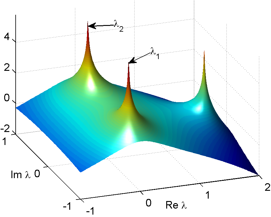
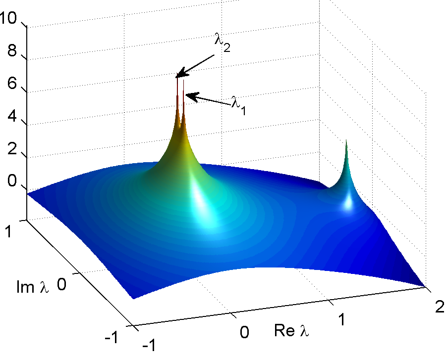
(a)	(b)
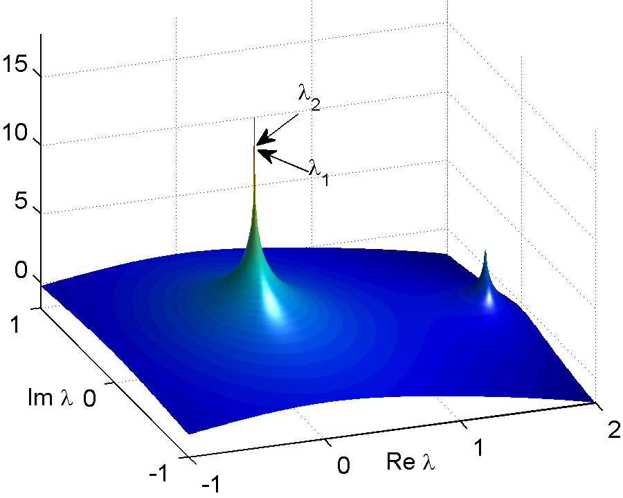
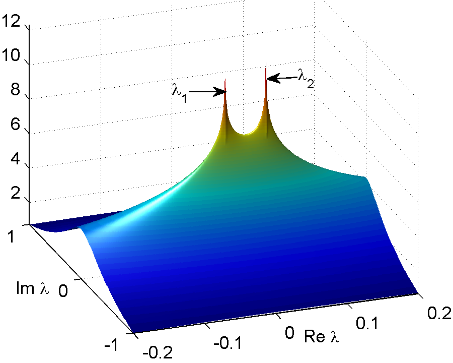
(c)	(d)

Figure 4.1. Graphs of the function $-\log\left|\Phi_{M}\right|$ from Example 4.8. On (a) the peaks on the left show the position of $\lambda_{1}$ and $\lambda_{2}$ when $s=0.956$. On (b) at $s=0.9995$ it is possible to see that the peaks on the left are closer to each other. On (c) the peaks of $\lambda_{1}$ and $\lambda_{2}$ are near to coalesce into a double eigenvalue at $s=0.9999006472847$, and finally on (d) $\lambda_{1}$ and $\lambda_{2}$ are two different real eigenvalues at $s=0.99999$.

4.4. The argument principle

Since the left-hand side of equation (4.13) is an analytic function with respect to $\lambda$, it is possible to apply the argument principle to locate its zeros and compute their order. Of course, in the case when an approximate characteristic function is just a polynomial as in (4.15), various methods of accurate localization of zeros are known and the usage of the argument principle can be excessive. Nevertheless even in this case the argument principle can be useful. As we already know only several roots of the polynomial (4.15) are approximations of the eigenvalues, all other roots appear due to the truncation of the series (4.13). The localization of several roots closest to the origin using the argument principle followed by several Newton iterations can be faster than the localization of all the roots by some general-purpose method. Moreover for more general boundary conditions, e.g., involving multiplication by an analytic function of $\lambda$, the approximate characteristic function may not be a polynomial, and the argument principle becomes even more useful (see, e.g., [6, 14, 53]). The argument principle consists in the following, see, e.g., [10].

Theorem 4.9 (The argument principle).

Let $f$ be an analytic function in a domain $G$ with zeros $z_{1}$, $z_{2}$,…,$z_{n}$ counted according to their multiplicity. If $\gamma$ is a simple closed rectifiable curve in $G$, contractible to a point in $G$ and not passing through $z_{1}$, $z_{2}$,…,$z_{n}$, then

(4.18) $$\frac{1}{2\pi i}\ointop_{\gamma}\frac{f^{\prime}(z)}{f(z)}dz=\sum_{k=1}^{n}n(\gamma;z_{k}),$$

where $n(\gamma;z_{k})$ is the winding number of $\gamma$ around $z_{k}$.

This theorem applied to the approximate characteristic function (4.15) in a domain restricted by the Rouché theorem (see the discussion above) allows one to find a precise number of eigenvalues and can even be used for their accurate location. We illustrate this approach in the next example for which a routine in MATLAB was written locating positions of zeros of the approximate characteristic function (4.15) by computing the argument change using $4000$ points along rectangular contours $\gamma$. If the argument change along certain $\gamma$ is zero the program considers another rectangular contour. Otherwise the program divides the rectangle into two smaller rectangles and calls the routine again on each rectangle until a desired tolerance is achieved. The program evaluates (4.18) over the final contour $\gamma$ to find the order of the zero and also refines the position of the zero by the well known residue formula (see e.g. [6, 30])

$$z_{k}=\frac{1}{2\pi iN(z_{k})}\ointop_{\gamma}\frac{z\Phi_{M}^{\prime}\left(z\right)}{\Phi_{M}\left(z\right)}dz,$$

where $N(z_{k})$ is the multiplicity of the zero $z_{k}$.

Example 4.10.

Consider the Zakharov-Shabat system with the potential (4.17). We compute the polynomial (4.15) with $M=100$ and present on Figure 4.2 the illustration of the work of the described algorithm. The shadowed areas contain the corresponding eigenvalues. Eigenvalues $\lambda_{1}$ and $\lambda_{2}$ get closer to each other and then separate. The plots illustrate the convergence of the described procedure to the approximate eigenvalues presented in Table 2.

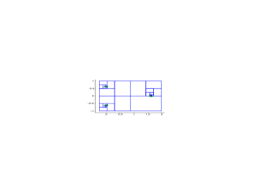
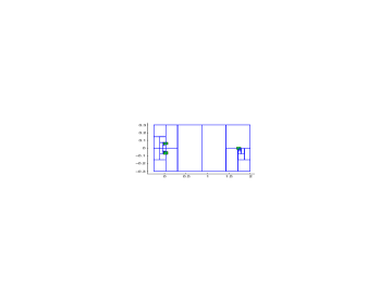
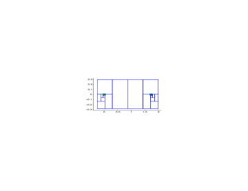
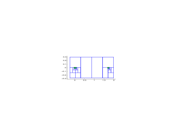
Figure 4.2. Illustration of the algorithm based on the argument principle in Example 4.10 for $s=0.956$ (top left), $s=0.9995$ (top right), $s=0.9999006472847$ (bottom left) and $s=0.99999$ (bottom right). Shadowed rectangles mark positions of the eigenvalues.

$s$	$\lambda_{1,2}$	$\lambda_{3}$
$0.956$	$0.0124269786\pm 0.6259290726i$	$1.6264287578+2\cdot 10^{-15}i$
$0.9995$	$0.0299931318\pm 0.0606462518i$	$1.7346285373-1.5\cdot 10^{-14}i$
$0.9999006472847$	$0.0301630556+3.9\cdot 10^{-15}i$, double eigenvalue	$1.7356369172-2\cdot 10^{-15}i$
$0.99999$	$0.0588404994+3.1\cdot 10^{-14}i$, $0.0015563906-2.8\cdot 10^{-14}i$	$1.7358620206+10^{-15}i.$

Table 2. Eigenvalues behavior depending on the parameter $s$ in Example 4.8.

4.5. Zakharov-Shabat systems with complex potentials.

In this subsection we compare the performance of the SPPS method with the results presented in [6, 49] where the semi-classical scaling of the non-self-adjoint Zakharov-Shabat scattering problem

(4.19) $$i\epsilon v_{x} = q\omega+\Lambda\upsilon$$

(4.20) $$i\epsilon\omega_{x} = q^{*}\upsilon-\Lambda\omega,$$

is considered, see also [20]. The potential function $q$ is of the form

(4.21) $$q(x) = A(x)e^{iS(x)/\epsilon}.$$

Considering notations $Q=\frac{i}{\epsilon}q^{*}$ and $\lambda=-\frac{i}{\epsilon}\Lambda$ one obtains the Zakharov-Shabat system (4.1), (4.2).

In order to apply the results of Subsections 4.2 and 4.3 we approximate the potential $q$ by a function compactly supported on $[-a,a]$. If $a$ is chosen to be sufficiently large the error due to this truncation of the potential is sufficiently small.

Example 4.11 ([6]).

Consider the functions

$$A(x)=\operatorname{sech}(2x),\qquad S(x)=\operatorname{sech}(2x)$$

for the potential (4.21). We approximated the potential with

$$\hat{q}(x)=\begin{cases}A(x)e^{iS(x)/\epsilon},&-a\leq x\leq a,\\ 0,&\text{ otherwise}\end{cases}$$

for $a=10$. The approximate eigenvalues obtained by the SPPS method for various values of $\epsilon$ are shown on Figure 4.3 and agree with the results from [6]. The presented results were obtained with the help of the spectral shift technique in Matlab using machine precision arithmetics, $M=250$ and 100000 points for the computation of the formal powers. For the smaller values of $\epsilon$ considered in [6] the SPPS method required to use high-precision arithmetics due to high oscillatory potential $q$ and nearly vanishing particular solution $u_{0}$. We chose not to include these numerical experiments.

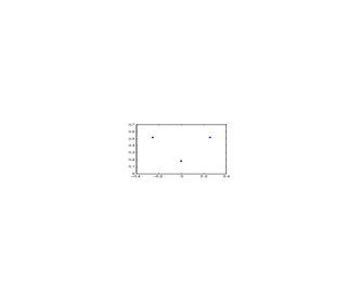
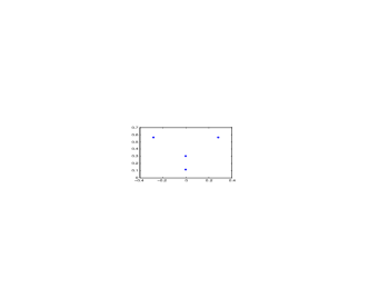
(a) $\epsilon$=0.2		(b) $\epsilon$=0.159
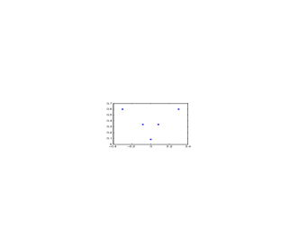
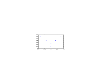
(c) $\epsilon$=0.126		(d) $\epsilon$=0.1
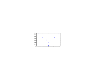
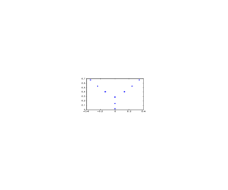
(e) $\epsilon$=0.0794		(f) $\epsilon$=0.063

Figure 4.3. Eigenvalue locations from Example 4.11 for $\epsilon$=0.2, 0.159, 0.126, 0.1, 0.0794 and 0.063.

Example 4.12.

In [49] the Zakharov-Shabat system (4.19), (4.20) with the potential (4.21) was considered for

$$A(x)=-\operatorname{sech}x,\qquad S^{\prime}(x)=-\mu\tanh x.$$

This potential is interesting because an exact formula for its eigenvalues is known and is given by

$$z_{n}=i\left(\sqrt{1-\frac{1}{4}\mu^{2}}-\varepsilon\left(n-\frac{1}{2}\right)\right),$$

where the index $n$ ranges strictly over the positive integers that satisfy

(4.22) $$n(\mu,\varepsilon)<\frac{1}{\varepsilon}\sqrt{1-\frac{\mu^{2}}{4}}+\frac{1}{2}.$$

Examples of the absolute error of the SPPS method for various values of $\mu$ and $\epsilon$ for this example are given in Table 3.

$\mu$	$\epsilon$	Number of eigenvalues according to (4.22)	Eigenvalues	Abs. error
$0.5$	$0.5$	$2$	$0.218245870595339i$ $0.718245836551895i$	$3.4\cdot 10^{-8}$ $5.5\cdot 10^{-14}$
$1$	$0.4$	$2$	$0.266025403665342i$ $0.666025403780913i$	$1.6\cdot 10^{-11}$ $1.8\cdot 10^{-12}$
$0.5$	$0.3$	$3$	$0.218245836882759i$ $0.518245836565527i$ $0.818245836562013i$	$1.2\cdot 10^{-11}$ $9.3\cdot 10^{-12}$ $6.9\cdot 10^{-12}$
$0.5$	$0.2$	$5$	$0.068246698084900i$ $0.268245836829048i$ $0.468245836567762i$ $0.668245836561404i$ $0.868245836536161i$	$2.9\cdot 10^{-9}$ $2.7\cdot 10^{-10}$ $1.4\cdot 10^{-9}$ $8.2\cdot 10^{-11}$ $3.4\cdot 10^{-12}$
$1$	$0.15$	$6$	$0.791025403810370i$ $0.641025403330507i$ $0.491025404649274i$ $0.341019810999524i$ $0.191026126515883i$ $0.041103889485868i$	$7.3\cdot 10^{-11}$ $1.8\cdot 10^{-10}$ $3.5\cdot 10^{-9}$ $5.8\cdot 10^{-6}$ $1.0\cdot 10^{-7}$ $2.1\cdot 10^{-5}$
$1$	$0.13$	$7$	$0.801025400788594i$ $0.671025403049713i$ $0.541025417533800i$ $0.411024735536490i$ $0.281025134994191i$ $0.151030141516677i$ $0.028942251261828i$	$6.7\cdot 10^{-8}$ $3.1\cdot 10^{-9}$ $1.3\cdot 10^{-8}$ $7.8\cdot 10^{-5}$ $1.3\cdot 10^{-7}$ $1.0\cdot 10^{-6}$ $2.7\cdot 10^{-3}$
$1$	$0.12$	$7$	$0.806025211476463i$ $0.686025403243744i$ $0.566025442436003i$ $0.446080832925892i$ $0.326025177679161i$ $0.206028821238862i$ $0.085971656937961i$	$4.0\cdot 10^{-6}$ $8.8\cdot 10^{-9}$ $1.3\cdot 10^{-7}$ $2.7\cdot 10^{-6}$ $2.8\cdot 10^{-6}$ $5.9\cdot 10^{-6}$ $8.0\cdot 10^{-5}$
$0.5$	$0.12$	$8$	$0.913160602214353i$ $0.788245879788585i$ $0.668245834591005i$ $0.548245717744945i$ $0.428227707506773i$ $0.308246463131394i$ $0.188245728430750i$ $0.068265536390608i$	$1.1\cdot 10^{-2}$ $1.3\cdot 10^{-7}$ $1.8\cdot 10^{-4}$ $8.5\cdot 10^{-8}$ $2.6\cdot 10^{-5}$ $6.7\cdot 10^{-7}$ $1.0\cdot 10^{-6}$ $1.2\cdot 10^{-5}$

Table 3. Eigenvalue errors from Example 4.12.

5. Relationship with the Dirac system

A relation between the one-dimensional stationary Dirac system from relativistic quantum theory and a quadratic Sturm-Liouville pencil can be established as follows. Consider the following canonical form of the Dirac system (see, e.g., [39, section 7])

$$y_{2}^{\prime}+\left(v(x)+\lambda\right)y_{1} =Ey_{1},$$

$$-y_{1}^{\prime}+(v(x)-\lambda)y_{2} =Ey_{2}.$$

Here $v$ is a potential, $\lambda$ corresponding to the mass of a particle is a spectral parameter and the constant $E$ is a fixed energy. Adding and subtracting the equations one obtains the system

$$u^{\prime}+\left(v-E\right)w =\lambda u,$$

$$w^{\prime}-\left(v-E\right)u =-\lambda w$$

for the functions $u=y_{2}-y_{1}$ and $w=y_{2}+y_{1}$. Supposing $v-E\neq 0$ on the domain of interest, it is easy to see from the second equality that $u=\frac{\lambda w+w^{\prime}}{v-E}$. Substituting this expression into the first equality one obtains an equation of the form (2.1):

$$\left(\frac{w^{\prime}}{v-E}\right)^{\prime}+\left(v-E\right)w=\lambda^{2}\frac{w}{v-E}+\lambda\left(\frac{1}{v-E}\right)^{\prime}w.$$

Analogously to what was presented in the preceding section for the Zakharov-Shabat system the SPPS representation for the solutions of the one-dimensional Dirac system as well as for the characteristic equations of corresponding spectral problems can be obtained.

6. A spectral problem for the equation of a smooth string with a distributed friction

The equation for the transverse displacement $u(x,t)$ of a string in an inhomogeneous absorbing medium (see, e.g., [3, 19, 29]) which extends in the $x$-direction from $x=0$ to $x=l$ with the characteristic parameters $c(x)>0$, $b(x)>0$ and the characteristic of absorption $\Gamma(x)$, has the form

(6.1) $$\frac{\partial}{\partial x}\left(c(x)\frac{\partial u}{\partial x}\right)-b(x)\frac{\partial^{2}u}{\partial t^{2}}-\Gamma(x)\frac{\partial u}{\partial t}=0.$$

The following condition expresses the hypothesis that the medium is totally reflecting at $z=0$:

(6.2) $$u(0,t)=0.$$

For a wave of frequency $\lambda$, i.e., for $u(x,t)=y(\lambda,x)e^{-i\lambda t}$, (6.1) and (6.2) take the form

(6.3) $$\begin{cases}\dfrac{\partial}{\partial x}\left(c(x)\dfrac{\partial y}{\partial x}\right)+\lambda^{2}b(x)y+i\lambda\Gamma(x)y=0,\\ y(\lambda,0)=0.\end{cases}$$

The equation in (6.3) is of the form (2.1). For numerical examples we will consider $c\equiv 1$, and the absorption $i\Gamma(x)=:2a(x)$ , i.e.,

(6.4) $$y^{\prime\prime}=2a(x)\lambda y+b(x)\lambda^{2}y$$

with the boundary conditions

(6.5) $$y(0)=y(1)=0.$$

6.1. Solution using the SPPS method

Equation (6.4) is a quadratic Sturm-Liouville pencil with $p=1$, $q=0$, $r_{1}=2a$ and $r_{2}=b$.

Take $x_{0}=0$ and $u_{0}=1$ for the SPPS method of Theorem 2.1. Due to the boundary conditions (6.5) we have that $c_{1}=0$. Then the characteristic equation of the problem (6.4), (6.5) has the form

$$\sum_{n=0}^{\infty}\lambda^{n}X^{\left(2n+1\right)}(1)=0,$$

and hence we are interested in locating zeros of the polynomial

(6.6) $$\Phi_{M}\left(\lambda\right)=\sum_{n=0}^{M}\lambda^{n}X^{\left(2n+1\right)}(1)$$

which approximate the eigenvalues of the problem.

In the following numerical examples the recursive integrals $X^{(n)}$ and $\widetilde{X}^{(n)}$ were calculated using the Newton-Cottes 6 point integration formula of 7-th order. On each step for the integration (if not specified explicitly) we took 100000 equally spaced sampling points on the segment $[0,1]$.

Example 6.1.

Consider equation (6.4) with $a=1$ and $b=1$. This is the case of a constant damping of a vibrating string. The exact characteristic equation [12] has the form $\lambda^{2}+2\lambda=-n^{2}\pi^{2}$, that is,

$$\lambda_{\pm n}=-1\pm\sqrt{1-n^{2}\pi^{2}},\qquad n=1,2,\ldots.$$

Approximation of the roots of the polynomial (6.6) by means of the routine roots of Matlab, with the machine precision arithmetic and $M=100$ delivers the results presented in the second column of Table 4. The same procedure but with the 256-digit precision arithmetic in Mathematica delivers the results presented in the third column of Table 4. As it can be appreciated, the first several eigenvalues are computed with a considerably better accuracy meanwhile the accuracy of higher computed eigenvalues does not change significantly. Doubling the number of the used formal powers delivers twice as many eigenvalues preserving the precision of the first eigenvalues and improving the precision of the forthcoming ones.

Eigenvalue	Abs. error, machine prec.	Abs. error, 256-digit prec. ($M=100$)	Abs. error, 256-digit prec. ($M=200$)	Abs. error, machine precision with spectral shift ($M=100$)
$\lambda_{\pm 1}$	$1.3\cdot 10^{-12}$	$1.4\cdot 10^{-29}$	$1.4\cdot 10^{-29}$	$6.2\cdot 10^{-13}$
$\lambda_{\pm 2}$	$1.8\cdot 10^{-13}$	$1.8\cdot 10^{-27}$	$1.8\cdot 10^{-27}$	$3.0\cdot 10^{-13}$
$\lambda_{\pm 3}$	$3.9\cdot 10^{-13}$	$3.0\cdot 10^{-26}$	$3.0\cdot 10^{-26}$	$4.0\cdot 10^{-14}$
$\lambda_{\pm 4}$	$4.5\cdot 10^{-12}$	$2.3\cdot 10^{-25}$	$2.3\cdot 10^{-25}$	$4.1\cdot 10^{-13}$
$\lambda_{\pm 5}$	$1.7\cdot 10^{-10}$	$1.1\cdot 10^{-24}$	$1.1\cdot 10^{-24}$	$1.6\cdot 10^{-13}$
$\lambda_{\pm 6}$	$3.7\cdot 10^{-9}$	$3.8\cdot 10^{-24}$	$3.8\cdot 10^{-24}$	$2.1\cdot 10^{-13}$
$\lambda_{\pm 7}$	$3.6\cdot 10^{-8}$	$1.1\cdot 10^{-23}$	$1.1\cdot 10^{-23}$	$2.5\cdot 10^{-13}$
$\lambda_{\pm 8}$	$3.3\cdot 10^{-7}$	$2.5\cdot 10^{-20}$	$2.9\cdot 10^{-23}$	$2.6\cdot 10^{-13}$
$\lambda_{\pm 9}$	$1.9\cdot 10^{-5}$	$4.5\cdot 10^{-15}$	$6.6\cdot 10^{-23}$	$1.8\cdot 10^{-13}$
$\lambda_{\pm 10}$	$4\cdot 10^{-4}$	$2.3\cdot 10^{-10}$	$1.4\cdot 10^{-22}$	$2.4\cdot 10^{-13}$
$\lambda_{\pm 11}$	$4\cdot 10^{-3}$	$4.2\cdot 10^{-6}$	$2.7\cdot 10^{-22}$	$3.0\cdot 10^{-13}$
$\lambda_{\pm 12}$	$3.1\cdot 10^{-2}$	$3.6\cdot 10^{-2}$	$4.9\cdot 10^{-22}$	$3.0\cdot 10^{-13}$
$\lambda_{\pm 13}$	$1.5$	$1.9$	$8.6\cdot 10^{-22}$	$1.8\cdot 10^{-13}$
$\lambda_{\pm 15}$			$2.3\cdot 10^{-21}$	$1.2\cdot 10^{-13}$
$\lambda_{\pm 20}$			$2.4\cdot 10^{-17}$	$7.1\cdot 10^{-14}$
$\lambda_{\pm 25}$			$2.9$	$1.6\cdot 10^{-13}$
$\lambda_{\pm 35}$				$9.0\cdot 10^{-13}$
$\lambda_{\pm 50}$				$1.9\cdot 10^{-11}$
$\lambda_{\pm 70}$				$7.8\cdot 10^{-10}$
$\lambda_{\pm 100}$				$4.0\cdot 10^{-7}$

Table 4. Eigenvalue errors from Example 6.1.

This shows that the usage of arbitrary precision arithmetic allows one to approximate more accurately the formal powers and the first eigenvalues, to obtain several additional eigenvalues. Meanwhile the spectral shift technique described in Section 3 permits to enhance the accuracy of the obtained eigenvalues as well as to calculate higher order eigenvalues even in machine precision.

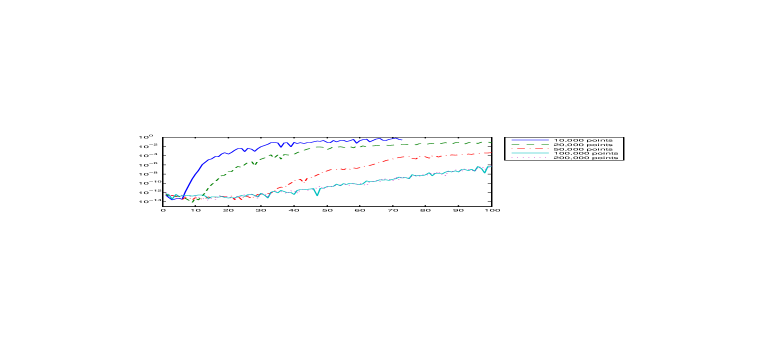
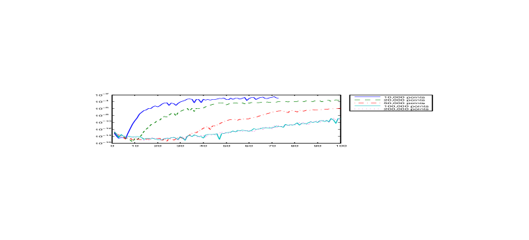
Figure 6.1. The plots of absolute (above) and relative (below) errors of the eigenvalues from Example 6.1 computed by means of the SPPS method using different numbers of points for calculating recursive integrals. The axis of abscissas corresponds to the ordinal number of the eigenvalue.

We used values $\widetilde{\lambda}_{n}=-1-(0.1+3i)n$ for the spectral shifts, on each step computing 201 formal powers, i.e., we took $M=100$ in (6.6), and evaluating the new particular solution in terms of these formal powers and the SPPS representation. The roots of (6.6) closest to the current spectral shift were stored as approximate eigenvalues. The results obtained with the spectral shift procedure are presented in the fifth column of Table 4. The eigenvalues were computed using the machine precision. A significant improvement in the accuracy and in the number of the found eigenvalues can be appreciated.

We verified the dependence of the eigenvalue errors on the number $N$ of points used for calculation of the recursive integrals. The plots of the absolute and relative errors of the eigenvalues for different values of $N$ obtained using the spectral shift technique described above are presented on Fig. 6.1. The increment of the value of $N$ to 100000 leads to the improvement of the eigenvalues accuracy, meanwhile further increment of $N$ does not change it significantly. The slow growth of the error for $N=100000$ is due to the increasing distance between the values $\widetilde{\lambda}_{n}$ used for the spectral shift and the eigenvalues. The observed rapid growth of the error starting from some particular eigenvalue index for smaller values of $N$ can be explained recalling that the higher index eigenfunctions as well as the solutions for close values of the spectral parameter are highly oscillatory, i.e., have large derivatives, and taking into account the error formula of Newton-Cottes integration rule (see [13, §2.4 and (2.5.26)]).

In the next example we present a problem with variable coefficients and illustrate the dependence of the approximate eigenvalues precision on the truncation parameter $M$ in (6.6).

Example 6.2.

Consider equation (6.4) with $a=x^{2}$ and $b=1$. The exact characteristic equation for this problem is

(6.7) $$\begin{split}&2^{\frac{\lambda^{\frac{3}{2}}}{2\sqrt{2}}}\Gamma\left(\frac{1}{8}\left(6+\sqrt{2}\lambda^{\frac{3}{2}}\right)\right)\operatorname{D}_{\frac{1}{4}\left(-2-\sqrt{2}\lambda^{\frac{3}{2}}\right)}\left(2^{\frac{3}{4}}\lambda^{\frac{1}{4}}\right)\\ &\qquad-\Gamma\left(\frac{1}{8}\left(6-\sqrt{2}\lambda^{\frac{3}{2}}\right)\right)\operatorname{D}_{\frac{1}{4}\left(-2+\sqrt{2}\lambda^{\frac{3}{2}}\right)}\left(2^{\frac{3}{4}}i\lambda^{\frac{1}{4}}\right)=0,\end{split}$$

where $\operatorname{D}$ is the parabolic cylinder function. For comparing the numerical results obtained by means of the SPPS method with the exact eigenvalues, Wolfram’s Mathematica FindRoot command was used for calculating the roots of (6.7).

On Fig. 6.2 we present the plots of the absolute errors of the computed eigenvalues using different values of $M$. All computations were performed in Matlab using machine precision, $100000$ points for evaluating recursive integrals and applying spectral shift technique with the spectral shifts $\lambda_{n}=-1-4\pi ni$, $n\leq 30$. As can be seen from the presented plots, the truncation parameter $M$ in (6.6) strongly affects the precision after the first spectral shift, meanwhile for the subsequent spectral shifts the precision is preserved. Starting from some particular value of $M$ the eigenvalue precision almost does not change, there is a small difference between $M=40$ and $M=50$ and no visible difference for $M=60$ (we did not include the errors for $M=60$ on the plots for this reason).

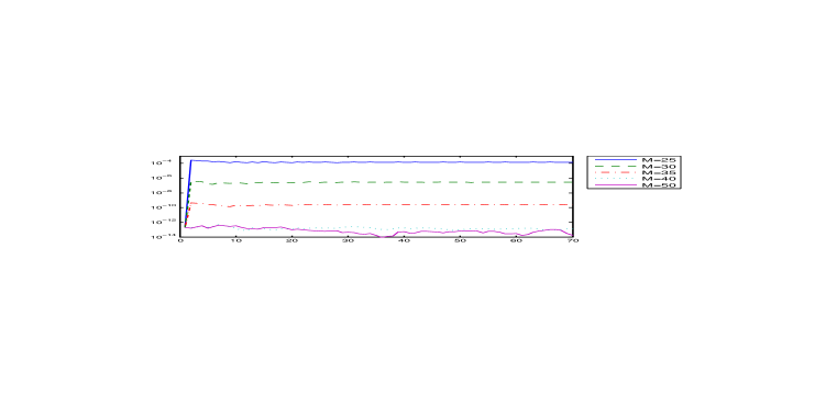
Figure 6.2. Absolute errors of the eigenvalues from Example 6.2 computed by means of the SPPS method using different number of formal powers. The axis of abscissae corresponds to the ordinal number of the eigenvalue.

References

- [1] M. J. Ablowitz and H. Segur, Solitons and the inverse scattering transform, Philadelphia: SIAM, 1981.
- [2] A. Agamaliyev and A. Nabiyev, On eigenvalues of some boundary value problems for a polynomial pencil of Sturm–Liouville equation, Appl. Math. Comput. 165 (2005) 503–515.
- [3] F. V. Atkinson, Discrete and continuous boundary problems, New York/London: Academic Press, 1964.
- [4] B. A. Babadzhanov, A. B. Khasanov and A. B. Yakhshimuratov, On the inverse problem for a quadratic pencil of Sturm-Liouville operators with periodic potential, Differ. Equ. 41 (2005) 310–318.
- [5] E. Bairamov and O. Çelebi, Spectral properties of the Klein-Gordon s-wave equation with complex potential, Indian J. Pure Appl. Math 28 (1997) 813–824.
- [6] J. C. Bronski, Semiclassical eigenvalue distribution of the non self-adjoint Zakharov-Shabat eigenvalue problem, Physica D, 97 (1996) 376–397.
- [7] R. Castillo, K. V. Khmelnytskaya, V. V. Kravchenko and H. Oviedo, Efficient calculation of the reflectance and transmittance of finite inhomogeneous layers, J. Opt. A: Pure Appl. Opt. 11 (2009), 065707.
- [8] R. Castillo P., V. V. Kravchenko, H. Oviedo and V. S. Rabinovich, Dispersion equation and eigenvalues for quantum wells using spectral parameter power series, J. Math. Phys. 52 (2011) 043522.
- [9] R. Castillo, V. V. Kravchenko and S. M. Torba, Spectral parameter power series for perturbed Bessel equations, Appl. Math. Comput. 220 (2013) 676–694.
- [10] J. B. Conway, Functions of one complex variable, Springer-Verlag, 1978.
- [11] R. Courant and D. Gilbert, Methods of mathematical physics. Vol. I., New York: Interscience Publishers, 1953.
- [12] S. Cox and E. Zuazua, The rate at which energy decays in a damped string, Commun. Partial Differ. Equ. 19 (1994) 213–243.
- [13] P. J. Davis and P. Rabinowitz, Methods of numerical integration. Second edition, New York: Dover Publications, 2007.
- [14] M. Dellnitz, O. Schütze and Q. Zheng, Locating all the zeros of an analytic function in one complex variable, J. Comput. Appl. Math. 138 (2002) 325–333.
- [15] M. Desaix, D. Anderson and M. Lisak, Variational approach to the Zakharov–Shabat scattering problem, Phys. Rev. E 50 (1994) 2253–2256.
- [16] L. Erbe, R. Mert and A. Peterson, Spectral parameter power series for Sturm–Liouville equations on time scales, Appl. Math. Comput. 218 (2012) 7671–7678.
- [17] B. Z. Guo and W. D. Zhu, On the energy decay of two coupled strings through a joint damper, J. Sound Vibr. 203 (1997) 447–455.
- [18] D. B. Hinton, A. K. Jordan, M. Klaus and J. K. Shaw, Inverse scattering on the line for a Dirac system, J. Math. Phys. 32 (1991) 3015–3030.
- [19] M. Jaulent, Inverse scattering problems in absorbing media, J. Math. Phys. 17 (1976) 1351–1360.
- [20] Y. Kim, L. Lee and G. D. Lyng, The WKB approximation of semiclassical eigenvalues of the Zakharov-Shabat problem, available at arXiv:1310.4145.
- [21] K. V. Khmelnytskaya, V. V. Kravchenko and J. A. Baldenebro-Obeso, Spectral parameter power series for fourth-order Sturm-Liouville problems, Appl. Math. Comput. 219 (2012) 3610–3624.
- [22] K. V. Khmelnytskaya, V. V. Kravchenko and H. C. Rosu, Eigenvalue problems, spectral parameter power series, and modern applications. Submitted, available at arXiv:1112.1633.
- [23] K. V. Khmelnytskaya and H. C. Rosu, A new series representation for Hill’s discriminant, Ann. Phys. 325 (2010) 2512–2521.
- [24] K. V. Khmelnytskaya and I. Serroukh, The heat transfer problem for inhomogeneous materials in photoacoustic applications and spectral parameter power series, Math. Meth. Appl. Sci. 36 (2013) 1878–1891.
- [25] K. V. Khmelnytskaya and T. V. Torchynska, Reconstruction of potentials in quantum dots and other small symmetric structures, Math. Meth. Appl. Sci. 33 (2010) 469–472.
- [26] M. Klaus and J. K. Shaw, Influence of pulse shape and frequency chirp on stability of optical solitons, Opt. Commun. 197 (2001) 491–500.
- [27] M. Klaus and J. K. Shaw, Purely imaginary eigenvalues of Zakharov-Shabat systems, Phys. Rev. E 65 (2002) 036607.
- [28] M. Klaus and J. K. Shaw, On the eigenvalues of Zakharov-Shabat systems, SIAM J. Math. Anal. 34 (2003) 759–773.
- [29] L. Kobyakova, Spectral problem generated by the equation of smooth string with piece-wise constant friction, Journal of Mathematical Physics, Analysis, Geometry, 8 (2012) 280–295.
- [30] P. Kravanja, T. Sakurai and M. Van Barel, On locating clusters of zeros of analytic functions, BIT Numer. Math. 39 (1999) 646–682.
- [31] V. V. Kravchenko, A representation for solutions of the Sturm-Liouville equation, Complex Var. Elliptic Equ. 53 (2008) 775–789.
- [32] V. V. Kravchenko, Applied pseudoanalytic function theory, Basel: Birkhäuser, 2009.
- [33] V. V. Kravchenko and R. M. Porter, Spectral parameter power series for Sturm-Liouville problems, Math. Meth. Appl. Sci. 33 (2010) 459–468.
- [34] V. V. Kravchenko and S. M. Torba, Transmutations and spectral parameter power series in eigenvalue problems, in Operator Theory: Advances and Applications, Vol. 228 (2013) 209–238.
- [35] V. V. Kravchenko and U. Velasco-García, Dispersion equation and eigenvalues for the Zakharov-Shabat system using spectral parameter power series, J. Math. Phys. 52 (2011) # 063517.
- [36] M. G. Krein and A. A. Nudelman, On direct and inverse problems for frequencies of boundary dissipation of inhomogeneous string, Dokl. Akad. Nauk SSSR, 247 (1979) 1046–1049.
- [37] M. G. Krein and A. A. Nudelman, On some spectral properties of an inhomogeneous string with dissipative boundary condition, J. Operat. Theor. 22 (1989) 369–395.
- [38] A. Laptev, R. Shterenberg and V. Sukhanov, Inverse spectral problems for Schrödinger operators with energy depending potentials, in CRM Proceedings and Lecture Notes, Vol. 4, (2007) 341–352.
- [39] B. M. Levitan and I. S. Sargsjan, Sturm-Liouville and Dirac operators, Kluwer Academic Pub., 1991.
- [40] J. Lin, Y. Li and X. Qian, The Darboux transformation of the Schrödinger equation with an energy-dependent potential, Phys. Lett. A 362 (2007) 212–214.
- [41] K. Liu and Z. Liu, Exponential decay of energy of vibrating strings with local viscoelasticity, Z. Angew. Math. Phys. 53 (2002) 265–280.
- [42] A. A. Nabiev, Inverse scattering problem for the Schrödinger-type equation with a polynomial energy-dependent potential, Inverse Probl. 22 (2006) 2055–2068.
- [43] I. M. Nabiev, The uniqueness of reconstruction of quadratic bundle for Sturm-Liouville operators, Proceedings of IMM of NAS of Azerbaijan 23 (2004) 91–96.
- [44] A. A. Nabiev and I. M. Guseinov, On the Jost solutions of the Schrödinger-type equations with a polynomial energy-dependent potential, Inverse Probl. 22 (2006) 55–67.
- [45] V. N. Pivovarchik, On spectra of a certain class of quadratic operator pencils with one-dimensional linear part, Ukr. Math. J. 59 (2007) 766–781.
- [46] N. Pronska, Reconstruction of energy-dependent Sturm-Liouville equations from two spectra, Integr. Equ. Oper. Theory 76 (2013) 403–419.
- [47] V. S. Rabinovich, R. Castillo-Pérez and F. Urbano-Altamirano, On the essential spectrum of quantum waveguides, Math. Meth. Appl. Sci. 36 (2013) 761–772.
- [48] J. Satsuma and N. Yajima, Initial value problems of one-dimensional self-modulation of nonlinear waves in dispersive media, Prog. Theor. Phys. Suppl. 55 (1974) 284–306.
- [49] A. Tovbis and S. Venakides, The eigenvalue problem for the focusing nonlinear Scrödinger equation: new solvable cases, Physica D 146 (2000) 150–164.
- [50] E. N. Tsoy and F. Kh. Abdullaev, Interaction of pulses in the nonlinear Schrödinger model, Phys. Rev. E 67 (2003) 056610.
- [51] C. Yang and A. Zettl, Half inverse problems for quadratic pencils of Sturm-Liouville operators, Taiwan. J. Math. 16 (2012) 1829–1846.
- [52] J. Yang, Nonlinear waves in integrable and nonintegrable systems, Philadelphia: SIAM, 2010.
- [53] X. Ying and I. N. Katz, A Reliable Argument Principle Algorithm to Find the Number of Zeros of an Analytic Function in a Bounded Domain, Numer. Math. 53 (1988) 143–163.
- [54] V. E. Zakharov and A. B. Shabat, Exact theory of two-dimensional self-focusing and one-dimensional self-modulation of waves in nonlinear media, Sov. Phys. JETP 34 (1972) 62–69.