Abundance Patterns in the Interstellar Medium of early-type galaxies observed with Suzaku

Abstract

We have analyzed 17 early-type galaxies, 13 ellipticals and 4 S0’s, observed with Suzaku, and investigated metal abundances (O, Mg, Si, and Fe) and abundance ratios (O/Fe, Mg/Fe, and Si/Fe) in the interstellar medium (ISM). The emission from each on-source region, which is 4 times effective radius, $r_{\rm e}$, is reproduced with one- or two- temperature thermal plasma models as well as a multi-temperature model, using APEC plasma code v2.0.1. The multi-temperature model gave almost the same abundances and abundance ratios with the 1T or 2T models. The weighted averages of the O, Mg, Si, and Fe abundances of all the sample galaxies derived from the multi-temperature model fits are 0.83 $\pm$ 0.04, 0.93$\pm$0.03, 0.80 $\pm$ 0.02, and 0.80$\pm$0.02 solar, respectively, in solar units according to the solar abundance table by Lodders (2003). These abundances show no significant dependence on the morphology and environment. The systematic differences in the derived metal abundances between the version 2.0.1 and 1.3.1 of APEC plasma codes were investigated. The derived O and Mg abundances in the ISM agree with the stellar metallicity within a aperture with a radius of one $r_{\rm e}$ derived from optical spectroscopy. From these results, we discuss the past and present SN Ia rates and star formation histories in early-type galaxies.

1 INTRODUCTION

The study on formation and evolution of early-type galaxies is one of the most important topics in modern astrophysics. The metal abundances of stars in these galaxies give us important constraints on theoretical models of their formation. In early-type galaxies, stellar mass loss and present type Ia supernovae (SNe Ia) have been providing metals in hot X-ray emitting interstellar medium (ISM). Thus, the metal abundance and their ratios in the ISM can provide a cumulative fossil record on the history of star formation.

Matsushita (2001) found that the X-ray luminosities in normal early-type galaxies which are not located at the center of group or cluster scale potential are consistent with the energy input from stellar mass loss. As a result, the hot ISM in these galaxies reflects almost instantaneous balance between heating and cooling. The mass of X-ray emitting ISM in early-type galaxies within 4 times the effective radius, $r_{\rm e}$, are about 0.1–1% of the stellar mass (Matsushita, 2001). The timescale for accumulation of this amount of hot ISM is smaller than $\sim$ 1 Gyr. Therefore, metal abundances in the ISM can constrain the present metal supply by SN Ia and stellar mass loss.

The ASCA satellite enabled us to measure the metal abundances in the ISM of early-type galaxies through spectral fitting of Fe-L lines. Since Fe in the ISM comes from stellar mass loss and SNe Ia, the Fe abundance in the ISM is expected to be a sum of the stellar metallicity and the contribution from SNe Ia, which is proportional to the ratio of SN Ia rate to stellar mass loss rate (see Matsushita et al. (2003) for details). Adopting the SN Ia rate recently estimated with optical observations, the resultant Fe abundance from SN Ia is at least 2 solar (e.g., Arimoto et al., 1997; Matsushita et al., 2003; Nagino & Matsushita, 2010; Konami et al., 2010; Loewenstein & Davis, 2010). However, the early measurements of ISM with ASCA showed that the metallicity is less than half a solar abundance (e.g., Awaki et al., 1994; Loewenstein et al., 1994; Mushotzky et al., 1994; Matsushita et al., 1994). Later, using the same ASCA data, the derived metal abundances in the ISM of these early-type galaxies have become $\sim$ 1 solar, considering uncertainties in the Fe-L atomic data (Arimoto et al., 1997; Matsushita et al., 1997, 2000), or employing a multi-temperature plasma model (Buote & Fabian, 1998). Using plasma codes with revised atomic data for the Fe-L lines, the Reflection Grating Spectrometer (RGS) onboard XMM-Newton, and the CCD detectors onboard Chandra and XMM-Newton yielded the Fe abundances in the ISM of $\sim$ 1 solar with a significant scatter. (e.g., Xu et al., 2002; Werner et al., 2009; Humphrey & Buote, 2006; Werner et al., 2006; Tozuka & Fukazawa, 2008; Ji et al., 2009). These Fe abundances are comparable to the stellar metallicity of these galaxies (Arimoto et al., 1997; Kobayashi & Arimoto, 1999), but still smaller than the expected values from SN Ia. Arimoto et al. (1997) have discussed various astrophysical aspects to the low Fe abundances in the ISM. Matsushita et al. (2000) suggested that SN Ia products in the ISM in early-type galaxies are lost to intergalactic space by their buoyancy. Tang & Wang (2010) also simulated the evolution of hot SN Ia ejecta, and found that they quickly reach a substantially higher outward velocity than the ambient medium. Loewenstein & Davis (2010) also suggested the ”effective” rate of SN Ia enrichment is less than the actual rate because SN Ia is not efficiently well-mixed into the ISM. There are, however, no clear theoretical or observational evidence which can resolve this discrepancy.

Since present star formation activity in early-type galaxies are generally low and SNe Ia rarely produce O or Mg, abundances of theses elements in the ISM should reflect stellar abundances. Using RGS detectors, the K$\alpha$ lines of O, Ne, and Mg from central regions of X-ray luminous early-type galaxies were clearly detected (Xu et al., 2002; Ji et al., 2009; Werner et al., 2009). The derived metal abundances of O, Ne, and Mg were about 0.5–1 solar. Using CCD detectors onboard Chandra and XMM, the abundance ratios such as O/Fe, Mg/Fe and Si/Fe were also derived (Humphrey & Buote, 2006; Tozuka & Fukazawa, 2008). The derived Mg/Fe and Si/Fe ratios are mostly consistent with the solar ratio, while the O/Fe ratios are often significantly smaller than the solar ratio. The Suzaku XIS (Koyama et al., 2007) has a good energy resolution at the O line energy, with a lower and more stable background level compared to the CCD detectors onboard Chandra and XMM-Newton and a larger effective area compared to the RGS detector. These advantage of Suzaku XIS can reduce the statistical and systematic errors in O and Mg abundance measurements. With Suzaku, the O, Mg, Si, and Fe abundances in the ISM in the entire region of several elliptical galaxies have been measured (e.g., Matsushita et al., 2007; Tawara et al., 2008; Hayashi et al., 2009; Loewenstein & Davis, 2010, 2012). The derived O/Fe, Mg/Fe, and Si/Fe ratios are close to that of the new solar abundance ratios determined by Lodders (2003). Suzaku also measured the metal abundances in the ISM of two S0 galaxies, NGC 4382 and NGC 1316 (Nagino & Matsushita, 2010; Konami et al., 2010). The O/Fe ratio in the ISM in NGC 4382 is smaller by a factor of two than those of the other early-type galaxies.

The stellar metallicity reflects the past activity of star formation. In addition, a longer formation time provides a higher concentration of trapped SNe Ia products to the stars. The stellar metallicity of the early-type galaxies has often been investigated in optical observations of their central regions using Mg and Fe absorption lines (e.g., Thomas et al., 2005; Bedregal et al., 2008; Walcher et al., 2009; Kobayashi & Arimoto, 1999; Kuntschner et al., 2010). They found that the metallicity and [$\alpha$/Fe] of stars in the core regions of early-type galaxies increase with the galactic mass. The derived stellar metallicity is about a 1 solar in giant elliptical galaxies, considering the gradient of strength of absorption lines (Arimoto et al., 1997; Kobayashi & Arimoto, 1999; Kuntschner et al., 2010). However, the observations of absorption lines are limited to $\sim r_{\rm e}$, which corresponds to a half light radius. In addition, there may be systematic uncertainties in the assumption of the age-population of stars, and in atomic physics. For example, Schiavon (2007) found that optical spectra of some early-type galaxies are better reproduced with a two-component age model, old and a small amount of young population. Then, the derived metal abundances also changed from a single component age model. With X-ray observations, we can measure the abundances of O and Mg of X-ray emitting ISM of the entire region of each galaxy. The metals in the hot ISM in early-type galaxies are a mixture of those from stars and recent SNe Ia and therefore, we can constrain stellar metallicity and their abundance pattern of the entire region of each galaxy. The relatively simple atomic data for X-ray lines and temperature structure of the ISM reduce the systematic uncertainties in the abundance measurements. Therefore, the X-ray measurements of metal abundances in the hot ISM and optical measurements of stellar metallicity are complementary.

In this paper, we performed uniform investigations of the metal abundances in the ISM of 17 early-type galaxies, 13 ellipticals and 4 S0’s, with Suzaku. This paper is structured as follows. In Section 2, we summarize observations of Suzaku. Sections 3 and 4 detail the data analysis and results. In Section 5, we investigated systematic differences between the v2.0.1 and v1.3.1 of the APEC plasma codes (Smith et al., 2001; Foster et al., 2012) on the derived elemental abundances. Section 6 gives a discussion of these results. Finally, in Section 7 we present our conclusion. Unless noted otherwise, we use the solar abundances in Lodders (2003), the v2.0.1 of the APEC plasma codes, and the quoted errors are for a 90% confidence interval for a single interesting parameter.

2 TARGETS AND OBSERVATIONS

We analyzed archival data of 17 early-type galaxies observed with Suzaku. The sample consists of 4 S0’s and 13 ellipticals, whose characteristics and observational log are summarized in Tables 1 and 2, respectively. Our sample includes only luminous early-type galaxies with $L_{K}>10^{11}L_{\odot}$. The luminosity of $10^{11}L_{\odot}$ in K band close to $L_{*}$, or the characteristic luminosity of the luminosity function by Schechter (1976) for clusters and groups galaxies by Lin & Mohr (2004). Nine galaxies are located in cluster environments (Virgo and Fornax clusters), while the others are either in the field or in small groups. NGC 1399 is the cD galaxy of the Fornax cluster, and NGC 4472 is the central galaxy of the south subgroup in the Virgo cluster. The temperature profiles of the ISM of NGC 1399, NGC 4472, NGC 4636, and NGC 5846 increase with radius (e.g. Matsushita et al., 2000; Nagino & Matsushita, 2009). These galaxies are the central objects of larger potential structure and have significantly higher ISM luminosities. Hereafter, we denote these galaxies as $X_{E}$ galaxies.

We used all available data of the galaxies in the sample with XIS. The XIS consists of three front-illuminated (FI: XIS0, XIS2 and XIS3) CCD cameras and one back-illuminated (BI: XIS1) CCD camera (Koyama et al., 2007). The XIS2 detector suffered catastrophic damage on November 2006. During observations of the sample galaxies, the XIS was operated in normal clocking mode (8 s exposure per frame), with the standard 5 $\times$ 5 and 3 $\times$ 3 editing mode.

Table 1: Galaxy sample in the Suzaku archive data.

Galaxy	$\rm type$	$\log~{}L_{\rm K}$	$r_{\rm e}$		$\sigma$	$N_{\rm H}$	$z$	$D$	$\log~{}L_{\rm X}$	Note
		$L_{\odot}$	arcsec	kpc	km/sec	1020cm-2		Mpc	erg/sec
NGC 720	-5.0	11.05	36.07	4.26	240	1.54	0.005821	20.3	40.46
NGC 1316	-2.0	11.56	80.75	9.61	250	1.89	0.005871	16.9	40.63	Fornax
NGC 1332	-2.0	11.02	28.00	2.88	319	2.23	0.005084	17.7	40.12
NGC 1399	-5.0	11.27	40.47	3.93	362	1.34	0.004753	16.9	41.13	$X_{\rm E}$, Fornax
NGC 1404	-5.0	11.07	23.83	3.15	245	1.36	0.006494	16.9	40.81	Fornax
NGC 1553	-2.0	11.08	65.63	4.79	185	1.50	0.003602	13.4	39.92
NGC 2300	-5.0	11.28	31.41	4.05	252	5.27	0.006354	31.0	41.90
NGC 3923	-5.0	11.57	49.79	5.87	241	6.21	0.005801	25.8	40.74
NGC 4125	-5.0	11.36	58.50	5.38	165	1.84	0.004523	24.2	40.67
NGC 4382	-2.0	11.33	54.59	2.73	187	2.52	0.002432	16.8	40.25	Virgo
NGC 4406	-5.0	11.35	104.02	1.77	250	2.62	0.000814	16.8	41.64	Virgo
NGC 4472	-5.0	11.63	104.02	7.07	302	1.66	0.003326	16.8	41.40	$X_{\rm E}$, Virgo
NGC 4552	-5.0	11.10	29.31	0.67	262	2.57	0.001134	16.8	40.62	Virgo
NGC 4636	-5.0	11.23	88.54	5.67	165	1.81	0.003129	17.0	41.46	$X_{\rm E}$, Virgo
NGC 4649	-5.0	11.50	68.73	5.22	343	2.20	0.003726	16.8	41.00	Virgo
NGC 4697	-5.0	11.53	71.97	6.05	165	2.12	0.004140	23.3	40.23
NGC 5846	-5.0	11.48	62.68	7.27	251	4.26	0.005717	28.5	41.72	$X_{\rm E}$

Table 2: Observational log.

Galaxy	$\rm ObsID$	$\rm Obsdate$	$\rm exposure$
			(ks)
NGC 720	800009010	2005-12-30	177.2
NGC 1316	801015010	2006-12-22	48.7
NGC 1332	805095010	2011-01-20	101.4
NGC 1399 & NGC1404	100020010	2005-09-13	76.1
NGC 1553	802050010	2007-11-25	98.7
NGC 2300	804030010	2010-02-08	37.1
	804030020	2010-02-10	52.6
NGC 3923	801054010	2006-06-13	115.8
NGC 4125	804047010	2009-09-29	104.1
NGC 4382	803005010	2008-06-21	99.1
NGC 4406	803043010	2009-06-19	101.8
NGC 4472	801064010	2006-12-03	121.0
NGC 4552	701037010	2006-12-03	20.4
NGC 4636	800018010	2005-12-06	79.2
NGC 4649	801065010	2006-12-29	224.0
NGC 4697	805041010	2011-01-14	102.3
NGC 5846	803042010	2008-07-28	155.9

3 DATA REDUCTION AND CONSTRUCTION OF SPECTRA

We processed the XIS data using the xispi and makepi ftool tasks and CALDB files of version 2012-07-03. The XIS data with the Earth elevation angles less than $5^{\circ}$ or the Day-Earth elevation angles less than $20^{\circ}$ were excluded. We also discarded data with time since south Atlantic anomaly passage of less than 436 sec. We created a 0.3–5 keV light curve for each sensor, with 256 s binning. All galaxies have no periods of anomalous event rates higher or less than $\pm 3\sigma$ from the mean. After this screening, the remaining good exposures were listed in Table 2. Event screening with cut-off rigidity was not performed. The spectral analysis was performed with HEAsoft version 6.12 and XSPEC 12.7.

We accumulated on-source spectra for each galaxy within 4 $r_{\rm e}$ centered on each galaxy. We used a accumulation radius of 3 $r_{\rm e}$ for NGC 1404, which is located near the cD galaxy, NGC 1399, of the Fornax cluster. To study the background emission, we also accumulated spectra over the entire XIS field of view excluding the on-source region (hereafter the background regions). The 4 $r_{\rm e}$ regions, which include most of stars in individual galaxies, are suitable for Suzaku analysis considering the point spread function. A larger accumulating region may suffer from a larger systematic uncertainties in the background emission including the cluster and group emission. Regions around luminous point sources were excluded from the analysis. The region around NGC 1404 was also excluded in the analysis of NGC 1399. We adopted an annular region of 3 $r_{\rm e}$–6 $r_{\rm e}$ from the center of NGC 1404 as the background region for NGC 1404. In Figure 1, we show XIS images with the on-source and the excluded regions for the analysis. Because the ISM emits little photons above 5 keV, to improve the photon statistics, we included corner regions illuminated by calibration sources, which have an emission peak at 5.9 keV.

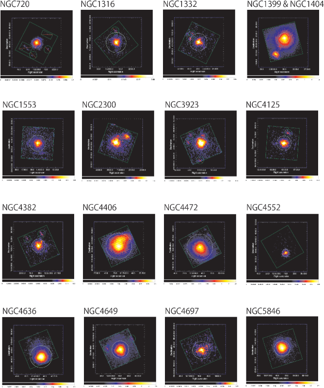
Figure 1: The 0.4–5 keV XIS1 images of our samples, smoothed with a $\sigma$=7$\farcs$5 Gaussian profile. Background components were not subtracted, and vignetting was not corrected in these images. The on-source regions are circular regions with a 4 $r{{}_{e}}$ radius shown in white circles. The green box and green circles represent the entire XIS field of view and the regions excluded from the analysis, respectively.

To subtract the non-X-ray background (NXB), we employed the Dark-Earth database using the xisnxbgen ftool task (Tawa et al., 2008). Redistribution matrix file (RMF) file were calculated using the xisrmfgen ftool task (Ishisaki et al., 2007), version 2011-07-02. The low energy transmission of the XIS optical blocking filters (OBF) has been decreased due to contamination on the filters (Koyama et al., 2007). The contaminant thickness has been evolved with time, and depends on the detector position. We used the ancillary response files (ARFs) generator, xissimarfgen ftool task (Ishisaki et al., 2007), version 2010-11-05, which includes transmission through the contaminant. Here, we used the observed XIS1 image of each galaxy for the emission components from the galaxy. For background components, we calculated ARF files in the same way but assuming a uniform sky emission. However, for the data of two X-ray luminous galaxies, NGC 4472 and NGC 4649 observed in December 2006 and all the data taken since 2008, there are still discrepancies between the data and model below 0.6 keV even using ARFs including the contaminant effect. Therefore, for these data, we used ARF files without including the effect of the contaminant. Instead, we multiplied “varabs” model, a photoelectric absorption model with variable abundances, by models used for spectral fitting. We summarized the treatment of contaminant and setting parameters of the “varabs” model in Appendix A.

4 Analysis and Results

4.1 Spectral fits with Single- and Two-Temperature models for the ISM

4.1.1 Estimation of the background spectra

In order to estimate background components, we first fitted the spectra of the background region. We used the following model for the emission from the background region: phabs $\times$ (power-law_CXB + apec_ETE + apec_MWH) + apec_LHB. In this model, “phabs” represents the Galactic absorption in the direction of each galaxy. After subtracting the NXB component, the emission of background regions consists of the cosmic X-ray background (CXB) and the emission from our Galaxy. We assumed a power-law model, “power-law_CXB” for the CXB component with a slope of $\Gamma=1.4$ (Kushino et al., 2002), and two APEC model components, “apec_LHB” and “apec_MWH”, for the Galactic emission. The “apec_LHB” component represents the sum of the solar wind charge exchange (SWCX) and local hot bubble (LHB), and the “apec_MWH” corresponds to the emission from Milky Way halo (MWH) (Yoshino et al., 2009). The metal abundances and redshift of “apec_MWH” and “apec_LHB” components were fixed at the solar value and zero, respectively. Though the temperatures of “apec_LHB” and “apec_MWH” models are basically set to free, for several galaxies with large error bars in temperatures of the Galactic components, we fixed theses temperatures at the values, which have $\chi^{2}$ minimum within a range of 0.05–0.3 keV and 0.3–0.6 keV for LHB and MWH, respectively.

The ISM emission may extend beyond each source region and galaxies located in clusters and groups are surrounded with intracluster medium (ICM). Therefore, we added an APEC component, “apec_ETE”, for these extra thermal emission (ETE). The metal abundances of “apec_ETE” components were free, but for NGC 1316, NGC 4406, and NGC4552, were fixed to 0.3 solar, because they are surrounded by the ICM (Tashiro et al., 2009; Shibata et al., 2001; Machacek et al., 2006). The redshift of “apec_ETE” component was fixed at that of each galaxy shown in Table 1. To fit the spectra of the background region, we need a two-temperature “apec_ETE” model for the ETE emission around NGC 4406, NGC 4472, and NGC 5846, and a two-temperature “vapec_ETE” model for NGC 1399, and a single-temperature“vapec_ETE” model for NGC 4636. The “vapec_ETE” model are variable abundance model adopting APEC plasma code (Smith et al., 2001). We summarized the derived parameters in Table 9 and 10 in Appendix B.

4.1.2 Simultaneously fit of the source and background spectra

The emission from each on-source region consists of the source emission from individual galaxies and the background emission. We assumed a following model as the source emission; phabs$\times$ (vapec_ISM + power-law_PS). Here, the “phabs” model corresponds to the photoelectric-absorption, whose column density was fixed to the Galactic value in the direction of each galaxy, shown in Table 1. The “vapec_ISM” model means thermal emission from the ISM. As shown in Figure 2, several emission lines seen around 0.5–0.6 keV, 0.6–0.7 keV, $\sim$ 1.3 keV, and $\sim$ 1.8 keV are identified with K$\alpha$ lines of O VII, O VIII, Mg XI, Si XIII, respectively. The emission bump around 0.7–1 keV mostly corresponds to the Fe-L complex, with smaller contributions by K-lines from Ne IX and Ne X and the Ni-L complex. We divided the metals into five groups as O, Ne, (Mg & Al), (Si, S, Ar, Ca), and (Fe & Ni), based on the metal synthesis mechanism of SNe, and allowed each group to vary. For luminous galaxies, NGC 1399, NGC 4406, NGC 4472, NGC 4649, and NGC 5846, we divided Si group as Si and (S, Ar, Ca). We set an upper limit of 5 solar for metal abundances. The abundances of He, C, and N were fixed to the solar value. The “power-law_PS” component represents the integrated discrete sources, with its photon index being fixed at 1.6 (e.g., Xu et al., 2005; Randall et al., 2006).

We used the same model in Section 4.1.1 for the emission from the background region. The metal abundance of the “apec_ETE” was fixed at the best-fit value, which is summarized in Table 9 (Appendix B), from fitting for the background regions. Only for NGC 1399 and NGC 4636, each metal abundances of ETE emission, which are represented by “vapec” models, are set to free, but limited within errors derived in Section 4.1.1, as shown in Table 10 (Appendix B).

We simultaneously fitted the spectra of the on-source and background regions to take into account background emission accurately. The background components (CXB, LHB, and MWH) were assumed to have the same surface brightness between the two regions. Except for NGC 1316, NGC 4406, and NGC 4552, the normalizations of the ETE components in source regions have been set to zero. We assumed the same surface brightness for the ETE components in the source and the background regions of these three galaxies, which are surrounded by the ICM emission. For NGC 1404, we subtracted the spectra of the annular region of 3–6 $r_{\rm e}$ as the background. We used energy ranges of 0.4–5.0 keV and 0.5–5.0 keV of the BI and FI detectors, respectively. Because there are known calibration issues of the Si edges in all XIS CCDs, an energy range of 1.84–1.86 keV is ignored (Koyama et al., 2007) in Suzaku spectra.

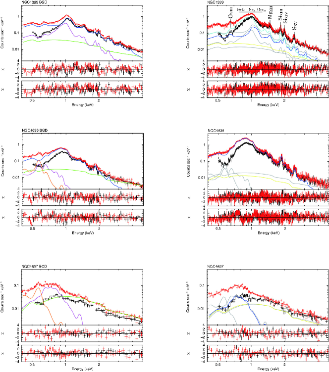
Figure 2: NXB-subtracted XIS0 (black) and XIS1 (red) spectra of each background region (left column), and those of NGC 1399 (1.05 keV), NGC4636 (0.80 keV), and NGC 4697 (0.25 keV) within the 4 $r_{\rm e}$ region (right column) in order from top to bottom, shown without removing the instrumental responses. The black and red lines show the best-fit model for the XIS0 and XIS1, respectively. For simplicity, only the model components for the XIS1 spectra are shown. The blue and light blue lines show the ISM components, yellow corresponds to the emission from discrete point sources, the magenta and orange lines show contributions from the Galactic emission by “apec_MWH” and “apec_LHB”, respectively, and the green lines for the CXB components. Panels under spectra show residuals of fit utilizing AtomDB v2.0.1 and v1.3.1 from the upper and the lower panels, respectively.

We used both one-temperature (1T) and two-temperature (2T) plasma models for the ISM emission to fit the spectra. For the 2T model, metal abundances of each element for the two temperature components were assumed to have a same value. The representative spectra fitted in this way are shown in Figure 2. The spectra of the other galaxies are shown in Appendix B. The 1T or 2T models for the ISM represent the spectra fairy well, expect for residual structures around 1.2 keV. Table 3 summarizes the derived ISM temperatures and $\chi^{2}$ for the spectral fits. With the 1T model fits, the temperatures of ISM of the sample galaxies range from 0.25 to 1.1 keV. As shown in Figure 3, the resultant $\chi^{2}$ fitted with the single- and two-temperature models for the ISM are almost the same, except for several galaxies. For ten galaxies, NGC 1316, NGC 1399, NGC 1404, NGC 1553, NGC 2300, NGC 3923, NGC 4125, NGC 4406, NGC 4472, and NGC 5846, we adopted the results of 2T model fits, since their F-test probabilities for adding the second temperature component are lower than 1%. Among them, NGC 1399, NGC 4472, and NGC 5846 are $X_{\rm E}$ galaxies, with positive temperature gradients (Nagino & Matsushita, 2009). NGC 4406 is an X-ray luminous galaxies with very complicated X-ray emission caused by ram-pressure stripping with the ICM in the Virgo cluster (e.g., Matsushita et al., 2000; Matsushita, 2001). The metal abundances derived from 1T and 2T model are summarised in Section 5.1. The reduced $\chi^{2}$ values with the 1T or 2T model fits are about 1.05–1.37 except for NGC 5846 whose reduced $\chi^{2}$ is 1.73. Considering only statistical errors, most of the fits are not acceptable. The large $\chi^{2}$ mainly caused by the residual structures around 1.2 keV. We discuss these residuals and possible systematic uncertainties in the Fe-L modeling in Section 5.3 and 5.4

Although the intensities of “power-law_PS” components have low impact to metal abundance measurements, we have checked these luminosities. The derived luminosities of “power-law_PS” components are compared to those derived from Chandra observations by Boroson et al. (2011). Overlapping their samples, the luminosities of “power-law_PS” components of NGC 1316, NGC 4125, NGC 4382, and NGC 4649, are good agreement with sum luminosities of low mass X-ray binaries and active galactic nuclei in Boroson et al. (2011).

Table 3: The ISM temperatures and $\chi^{2}$ derived from the 1T, 2T and multi-T model fits using APEC plasma code, v2.0.1. The flux ratios of high and low temperature ISM for galaxies whose best fit is 2T model.

Galaxy	kT (1T)	${\chi^{2}}$/d.o.f.	kT (2T)		flux ratio	${\chi^{2}}$/d.o.f.	${\chi^{2}}$/d.o.f.
	(keV)	(1T)	(keV)	(keV)	highT/lowT	(2T)	(Multi-T)
NGC 720	0.61${}^{+0.01}_{-0.01}$	745/545	0.62${}^{+0.07}_{-0.02}$	$<$0.41	$\cdots$	739/543	743/547
NGC 1316	0.65${}^{+0.02}_{-0.02}$	511/414	0.93${}^{+0.04}_{-0.04}$	0.45${}^{+0.05}_{-0.05}$	1.09	461/412	411/411
NGC 1332	0.60${}^{+0.02}_{-0.02}$	449/411	0.86${}^{+0.50}_{-0.10}$	0.53${}^{+0.09}_{-0.43}$	$\cdots$	445/409	447/412
NGC 1399	1.05${}^{+0.01}_{-0.01}$	3129/2023	1.74${}^{+0.22}_{-0.05}$	1.01${}^{+0.01}_{-0.01}$	0.39	2778/2021	2780/2028
NGC 1404	0.66${}^{+0.01}_{-0.01}$	447/407	0.72${}^{+0.08}_{-0.06}$	0.43${}^{+0.03}_{-0.02}$	3.64	434/405	435/406
NGC 1553	0.57${}^{+0.02}_{-0.02}$	535/415	0.64${}^{+0.09}_{-0.09}$	0.31${}^{+0.08}_{-0.08}$	0.85	516/412	523/415
NGC 2300	0.74${}^{+0.02}_{-0.02}$	579/442	4.06${}^{+1.30}_{-2.21}$	0.73${}^{+0.02}_{-0.02}$	0.33	566/440	578/443
NGC 3923	0.60${}^{+0.01}_{-0.01}$	752/547	0.41${}^{+0.04}_{-0.03}$	0.70${}^{+0.04}_{-0.08}$	0.94	719/545	722/547
NGC 4125	0.47${}^{+0.03}_{-0.03}$	525/408	0.59${}^{+0.17}_{-0.08}$	0.32${}^{+0.10}_{-0.07}$	0.91	497/406	497/410
NGC 4382	0.33${}^{+0.03}_{-0.02}$	435/413	$<$0.39	$<$0.26	$\cdots$	433/411	433/415
NGC 4406	0.84${}^{+0.01}_{-0.01}$	2612/2069	1.29${}^{+0.22}_{-0.07}$	0.81${}^{+0.01}_{-0.01}$	0.34	2537/2067	2586/2070
NGC 4472	1.04${}^{+0.01}_{-0.01}$	3288/2160	1.65${}^{+0.08}_{-0.09}$	1.00${}^{+0.01}_{-0.01}$	0.43	2549/2158	2549/2160
NGC 4552	0.65${}^{+0.04}_{-0.03}$	588/485	0.75${}^{+0.13}_{-0.11}$	0.38${}^{+0.22}_{-0.11}$	$\cdots$	583/483	583/487
NGC 4636	0.80${}^{+0.01}_{-0.01}$	3124/2298	0.61${}^{+0.03}_{-0.07}$	0.85${}^{+0.02}_{-0.03}$	$\cdots$	3115/2301	3114/2303
NGC 4649	0.86${}^{+0.01}_{-0.01}$	2630/2057	0.85${}^{+0.01}_{-0.01}$	$<$0.12	$\cdots$	2623/2055	2630/2057
NGC 4697	0.25${}^{+0.05}_{-0.03}$	514/412	$<$0.76	0.19${}^{+0.04}_{-0.05}$	$\cdots$	503/410	509/414
NGC 5846	0.76${}^{+0.01}_{-0.01}$	1110/567	0.88${}^{+0.01}_{-0.01}$	0.58${}^{+0.03}_{-0.03}$	1.69	976/565	976/566

Figure 3: Comparison of ${\chi^{2}}$ between the 1T and 2T or multi-T models. The dashed lines indicate the equal value between the two.

In order to examine the abundance ratios rather than their absolute vales, we calculated the confidence contours between the abundance of various metals (O, Ne, Mg, and Si) to that of Fe. The results are shown in Figure 4, where we also indicate 90%-confidence abundance of these metals relative to Fe with black dashed line. The elongated shape of the confidence contours indicates that the relative values were determined more accurately than the absolute values.

Figure 4: The confidence contours of the abundances of O, Ne, Mg, Si vs. Fe in solar units for NGC 1399 with the 2T model fits. The three contours represent the 68%, 90%, and 99% confidence ranges from inner to outer, respectively. The dashed lines show the 90%-confidence level of these metal abundances relative to Fe.

The resultant temperatures in the background components are consistent to those derived in Section 4.1.1 (Table 9). The derived of the Galactic components, MWH and LHB (and SWCX), are about 0.2–0.3 keV and 0.1 keV, respectively. These values are consistent with those derived for other sky regions without luminous sources observed with Suzaku (e.g., Yoshino et al., 2009).

4.2 Spectral fits with multi-temperature model for the ISM

The temperature gradients of the ISM within 4 $r_{e}$ in early-type galaxies have been reported with Chandra and XMM-Newton satellites (e.g., Nagino & Matsushita, 2009; Ji et al., 2009). X-ray luminous galaxies tend to have increasing temperature profiles, while others show constant or decreasing profile. We used a multi-temperature model (hereafter multi-T model) for the ISM and refitted the spectra in the same way as in Section 4.1. For galaxies which need the 2T model for the ISM, we fitted the spectra with a five-temperature model, and for the other galaxies, we used a three-temperature model. The difference of temperatures of the two neighboring components was fixed at 0.2 keV, and the temperature of the central temperature component was fixed to be the best-fit temperature derived from the 1T model fit or the intermediate value between the best-fit two temperatures derived from the 2T model fit. The multi-T model fit gave almost the same $\chi^{2}$ (Figure 3) and show similar residual structures with the 1T or 2T model fits.

Table 4: The O, Ne, Mg, Si, S and Fe abundances in the ISM derived from the multi-T model fits using APEC plasma code, v2.0.1.

Galaxy	O	Ne	Mg	Si	S	Fe
	(solar)	(solar)	(solar)	(solar)	(solar)	(solar)
NGC 720	1.09${}^{+0.38}_{-0.26}$	1.82${}^{+0.55}_{-0.38}$	1.16${}^{+0.37}_{-0.27}$	1.19${}^{+0.43}_{-0.30}$	=Si	1.05${}^{+0.28}_{-0.19}$
NGC 1316	0.92${}^{+0.54}_{-0.31}$	1.43${}^{+0.98}_{-0.60}$	0.89${}^{+0.65}_{-0.35}$	0.49${}^{+0.43}_{-0.26}$	=Si	0.79${}^{+0.44}_{-0.24}$
NGC 1332	3.19${}^{+1.81}_{-1.62}$	5.00${}^{+0}_{-2.25}$	3.76${}^{+1.24}_{-1.74}$	1.92${}^{+1.52}_{-1.16}$	=Si	2.52${}^{+1.15}_{-1.08}$
NGC 1399	1.01${}^{+0.17}_{-0.19}$	3.16${}^{+0.41}_{-0.41}$	1.64${}^{+0.16}_{-0.07}$	1.76${}^{+0.26}_{-0.11}$	1.30${}^{+0.28}_{-0.15}$	1.43${}^{+0.16}_{-0.08}$
NGC 1404	1.20${}^{+0.58}_{-0.36}$	1.67${}^{+0.83}_{-0.58}$	0.89${}^{+0.44}_{-0.28}$	1.52${}^{+0.81}_{-0.51}$	=Si	1.27${}^{+0.47}_{-0.28}$
NGC 1553	5.00${}^{+0}_{-3.23}$	4.80${}^{+0.20}_{-3.48}$	3.23${}^{+1.77}_{-2.30}$	1 (fix)	=Si	4.77${}^{+0.23}_{-3.02}$
NGC 2300	1.02${}^{+0.50}_{-0.44}$	2.20${}^{+0.81}_{-0.76}$	1.04${}^{+0.45}_{-0.27}$	0.80${}^{+0.35}_{-0.22}$	=Si	0.60${}^{+0.21}_{-0.13}$
NGC 3923	1.21${}^{+0.94}_{-0.42}$	1.80${}^{+1.42}_{-0.76}$	1.46${}^{+1.14}_{-0.48}$	1.11${}^{+0.94}_{-0.51}$	=Si	1.26${}^{+0.87}_{-0.37}$
NGC 4125	0.49${}^{+0.28}_{-0.17}$	0.82${}^{+0.45}_{-0.27}$	0.50${}^{+0.31}_{-0.19}$	0.44${}^{+0.48}_{-0.33}$	=Si	0.60${}^{+0.25}_{-0.14}$
NGC 4382	0.83${}^{+0.50}_{-0.28}$	1.28${}^{+0.79}_{-0.44}$	1.12${}^{+0.80}_{-0.46}$	1 (fix)	=Si	1.29${}^{+0.75}_{-0.40}$
NGC 4406	0.80${}^{+0.19}_{-0.17}$	2.28${}^{+0.38}_{-0.36}$	0.79${}^{+0.09}_{-0.10}$	0.53${}^{+0.07}_{-0.03}$	0.79${}^{+0.07}_{-0.09}$	0.72${}^{+0.07}_{-0.06}$
NGC 4472	0.86${}^{+0.12}_{-0.10}$	2.07${}^{+0.20}_{-0.11}$	0.88${}^{+0.08}_{-0.07}$	0.96${}^{+0.06}_{-0.05}$	0.98${}^{+0.07}_{-0.07}$	0.86${}^{+0.05}_{-0.04}$
NGC 4552	1.08${}^{+1.04}_{-0.56}$	0.85${}^{+1.30}_{-0.85}$	0.95${}^{+0.78}_{-0.45}$	1 (fix)	=Si	0.83${}^{+0.50}_{-0.25}$
NGC 4636	0.73${}^{+0.07}_{-0.07}$	1.97${}^{+0.15}_{-0.15}$	0.88${}^{+0.06}_{-0.05}$	0.86${}^{+0.05}_{-0.05}$	=Si	0.80${}^{+0.04}_{-0.03}$
NGC 4649	0.87${}^{+0.12}_{-0.11}$	1.71${}^{+0.16}_{-0.15}$	0.80${}^{+0.08}_{-0.07}$	0.75${}^{+0.06}_{-0.05}$	0.85${}^{+0.09}_{-0.08}$	0.69${}^{+0.04}_{-0.04}$
NGC 4697	0.62${}^{+0.82}_{-0.29}$	1.95${}^{+1.98}_{-0.85}$	1 (fix)	1 (fix)	=Si	1.46${}^{+1.58}_{-0.61}$
NGC 5846	1.03${}^{+0.15}_{-0.12}$	2.14${}^{+0.24}_{-0.20}$	1.02${}^{+0.10}_{-0.09}$	0.98${}^{+0.09}_{-0.08}$	1.16${}^{+0.07}_{-0.13}$	0.84${}^{+0.06}_{-0.05}$

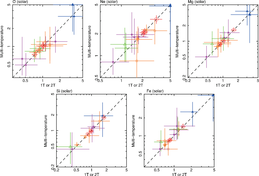
Figure 5: Comparison of abundances of O, Ne, Mg, Si, and Fe with the multi-T model and the 1T or 2T models. Statement of meanings of the symbols is shown in Figure 7.

4.3 Comparison of abundances derived with the 1T or 2T and multi-T models

The derived abundances with the multi-T model fits are summarized in Table 4. Figure 5 compares the resultant O, Ne, Mg, Si, and Fe abundances from the 1T or 2T models and multi-T model fits. For most of the cases, the multi-T model gave almost save values except for a few galaxies with large error bars. To study the temperature dependence of the differences between the abundances from the 1T or 2T and multi-T model fits, we divided galaxies into three groups, using the ISM temperature derived from the 1T model fits of $<0.4$ keV, 0.4–1.0 keV, and $>1.0$ keV. Then, we calculated weighted averages of the metal abundances and metal-to-Fe abundance ratios derived from the 1T or 2T models and the multi-T model fits for galaxies belong to each temperature group and the whole sample. The results are summarized in Figure 6 and Table 5. The weighted averages of O, Ne, Mg, Si, and Fe abundances and O/Fe, Ne/Fe, Mg/Fe, and Si/Fe ratios derived from the 1T or 2T and the multi-T model fits mostly agree well with each other within several %. For the galaxies with ISM temperature lower than 0.4 keV, the multi-T model tended to yield higher Fe abundances than the 1T or 2T models, although the error bars are very large.

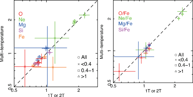
Figure 6: Comparison of the weighted averages of abundances (O, Ne, Mg, Si, and Fe; left) and abundance ratios (O/Fe, Ne/Fe, Mg/Fe, and Si/Fe; right) with the multi-T and the 1T or 2T models. The dashed lines indicate the equal value between two models.

Table 5: The weighted averages of abundances of O, Ne, Mg, Si, and Fe and O/Fe, Ne/Fe, Mg/Fe, and Si/Fe ratios for all the sample galaxies and those with ISM temperatures of $<0.4$ keV, 0.4–1.0 keV, $>1.0$ keV.

		All	$<$0.4 keV	0.4-1 keV	$>$1 keV
1T or 2T / v2.0.1	O	0.84$\pm 0.05$	0.63$\pm 0.26$	0.85$\pm 0.05$	0.90$\pm 0.10$
	Ne	1.89$\pm 0.07$	1.20$\pm 0.42$	1.87$\pm 0.08$	2.27$\pm 0.25$
	Mg	0.89$\pm 0.03$	1.02$\pm 0.53$	0.87$\pm 0.03$	0.99$\pm 0.08$
	Si	0.83$\pm 0.03$	$\cdots$	0.78$\pm 0.03$	1.07$\pm 0.07$
	Fe	0.79$\pm 0.02$	1.15$\pm 0.38$	0.76$\pm 0.02$	0.96$\pm 0.05$
	O/Fe	1.02$\pm 0.05$	0.57$\pm 0.25$	1.09$\pm 0.06$	0.94$\pm 0.09$
	Ne/Fe	2.21$\pm 0.07$	1.04$\pm 0.21$	2.41$\pm 0.08$	2.37$\pm 0.25$
	Mg/Fe	1.12$\pm 0.03$	0.88$\pm 0.37$	1.14$\pm 0.03$	1.05$\pm 0.06$
	Si/Fe	1.06$\pm 0.02$	$\cdots$	1.03$\pm 0.03$	1.12$\pm 0.04$
Multi-T / v2.0.1	O	0.83$\pm 0.04$	0.76$\pm 0.32$	0.82$\pm 0.05$	0.90$\pm 0.09$
	Ne	1.95$\pm 0.07$	1.37$\pm 0.56$	1.87$\pm 0.09$	2.21$\pm 0.14$
	Mg	0.93$\pm 0.03$	1.12$\pm 0.63$	0.87$\pm 0.04$	1.11$\pm 0.06$
	Si	0.80$\pm 0.02$	$\cdots$	0.81$\pm 0.03$	1.02$\pm 0.05$
	Fe	0.80$\pm 0.02$	0.75$\pm 0.18$	0.77$\pm 0.02$	0.93$\pm 0.04$
	O/Fe	0.95$\pm 0.05$	0.64$\pm 0.12$	1.05$\pm 0.06$	0.86$\pm 0.10$
	Ne/Fe	2.02$\pm 0.08$	1.02$\pm 0.18$	2.22$\pm 0.09$	2.35$\pm 0.21$
	Mg/Fe	1.12$\pm 0.03$	0.88$\pm 0.34$	1.13$\pm 0.03$	1.06$\pm 0.06$
	Si/Fe	1.00$\pm 0.03$	$\cdots$	1.01$\pm 0.03$	1.15$\pm 0.05$
1T or 2T / v1.3.1	O	0.62$\pm 0.03$	0.40$\pm 0.17$	0.60$\pm 0.04$	0.87$\pm 0.09$
	Ne	1.22$\pm 0.06$	0.78$\pm 0.29$	1.19$\pm 0.06$	1.84$\pm 0.22$
	Mg	0.87$\pm 0.03$	0.80$\pm 0.42$	0.82$\pm 0.03$	1.28$\pm 0.11$
	Si	0.98$\pm 0.03$	$\cdots$	0.93$\pm 0.03$	1.44$\pm 0.09$
	Fe	0.94$\pm 0.03$	1.33$\pm 0.46$	0.88$\pm 0.03$	1.37$\pm 0.08$
	O/Fe	0.60$\pm 0.03$	0.24$\pm 0.12$	0.63$\pm 0.03$	0.63$\pm 0.06$
	Ne/Fe	1.09$\pm 0.05$	0.57$\pm 0.12$	1.20$\pm 0.06$	1.37$\pm 0.17$
	Mg/Fe	0.91$\pm 0.02$	0.64$\pm 0.27$	0.91$\pm 0.02$	0.93$\pm 0.04$
	Si/Fe	1.00$\pm 0.02$	$\cdots$	0.98$\pm 0.03$	1.06$\pm 0.04$

4.4 Abundances and their ratios with the multi-T model fits

In Figure 7, we plotted the abundances of O, Mg, and Fe derived from the multi-T model fits against the 1T temperatures of ISM. The values of O, Mg, and Fe abundances are about 1 solar, with no significant dependence on the ISM temperature. Elliptical and S0 galaxies have similar values of O, Mg, and Fe abundances. These abundances also show no significant dependence on the environment. The weighted averages of the O, Mg, Si, and Fe abundances of all the sample galaxies derived from the multi-T model fits are 0.83 $\pm$ 0.04, 0.93$\pm$0.03, 0.80 $\pm$ 0.02, and 0.80$\pm$0.02 solar, respectively, in solar units (Table 5).

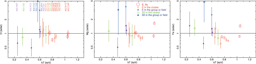
Figure 7: Abundances of O, Mg and Fe derived from the multi-T model fits. Closed and opened triangles (circles) show the abundance patterns of S0 (elliptical) galaxies in the field or group and cluster, respectively. The larger open circles correspond to X-ray luminous objects, or $X_{E}$ galaxies (Nagino & Matsushita, 2009). Solid lines represent the solar abundance (Lodders, 2003).

Figure 8 shows the O/Fe, Ne/Fe, Mg/Fe, and Si/Fe ratios plotted against the ISM temperature. These ratios are plotted in terms of number ratios, to avoid differences in different solar abundance tables. The derived O/Fe, Mg/Fe, and Si/Fe ratios are mostly consistent with the solar ratios, except for the O/Fe ratio in the ISM of an S0 galaxy, NGC 4382, with the ISM temperature of 0.33 keV, as reported by Nagino & Matsushita (2010). The weighted averages of the abundance ratios for each temperature group are also plotted in Figure 6 (right panel). Those of Mg/Fe and Si/Fe of all temperature groups are close to the solar ratio. Because of the low O/Fe ratio of NGC 4382, the weighted average of the O/Fe ratios of galaxies with ISM temperature below 0.4 keV is 0.64 $\pm$ 0.12 in unit of the solar ratio, which is smaller than those of the higher temperature groups. Again, there is no significant dependence on the morphology and environment of galaxies.

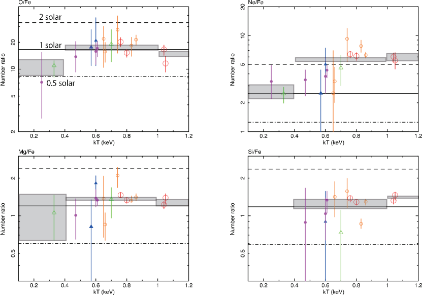
Figure 8: Abundance ratios of O, Ne, Mg, and Si to Fe derived from the multi-T model fits. Meanings of the symbols are the same as those in Figure 7. Solid, dashed, and dot-dashed lines represent the solar abundance (Lodders, 2003), twice, and half of solar ratios, respectively. Gray boxes show the weighted averages for the three temperature groups, summarized in Table 5.

The derived Ne/Fe ratios are about 2 in unit of the solar ratio, and NGC 4382 has a significantly smaller Ne/Fe ratio than the other galaxies by a factor of two (Figure 8). Since K-shell lines of Ne are hidden in the Fe-L region, the systematic uncertainties in the derived Ne abundances may be significant. We discuss the dependence on the Ne abundances on the version of atomic data at Section 5.

4.5 Effect of the He abundance in the ISM

The hot ISM in early-type galaxies are thought to be an accumulation of stellar mass loss, mainly from asymptotic giant branch (AGB) stars. As a result, the mass-loss products may have significantly higher He abundances. From optical observations of AGB stars, the measured He abundances are up to around 2.5 solar (Mello et al., 2012). Since a higher He abundance increases the continuum level, the assumption of the solar He abundance can yields an underestimation of the Fe abundance. To study the effect of the assumption of the He abundance in the ISM, we fitted the spectra in the same way in Section 4.1, changing the assumed He abundance from 1.2 to 3 solar. The derived metal abundances have a weak dependence on the He abundance, and the three solar He abundance gives a 10–30% higher metal abundances. Therefore, systematic uncertainties in the metal abundances caused by the uncertainty in the He abundance are relatively small.

5 SYSTEMATIC UNCERTAINTIES BY THE VERSION OF ATOMIC DATA

5.1 Comparison of metal abundances derived from 1T and 2T model

Using ASCA data, Buote & Fabian (1998) reported that spectral fits with a multi-temperature plasma model for the ISM in some luminous early-type galaxies gave larger metal abundances than those with a single temperature model. We plotted the derived Fe abundances from the 1T and 2T models using AtomDB v2.0.1 in Figure 9. The Fe abundances of some galaxies derived from the 2T model fits are higher than those derived from the 1T model by several tens of %, while there are X-ray luminous galaxies whose Fe abundances derived from the 1T and 2T model fits are nearly the same. The differences in the Fe abundances derived from the 1T and 2T model fits tend to be smaller than those reported by Buote & Fabian (1998), where a plasma code of MEKAL (Liedahl et al., 1995) was used. The differences in the adopted plasma codes, especially for the Fe-L lines, also affects the differences in the derived metal abundances as reported in previous studies (e.g., Loewenstein et al., 1994; Matsushita et al., 2000, 2007; Nagino & Matsushita, 2010). The hotter temperature component by Buote & Fabian (1998) have temperatures of a few keV, which may be come from accumulated emission of point sources.

We also plotted the derived O/Fe, Ne/Fe, Mg/Fe, and Si/Fe ratios in Figure 10. The derived ratios of O/Fe, Ne/Fe, Mg/Fe, and Si/Fe are consistent between the 1T and 2T models within error bars, although some galaxies have smaller O/Fe ratios from the 2T models compared to those from the 1T models.

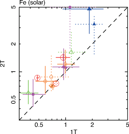
Figure 9: Comparison of abundances of Fe with the 1T model and 2T model. Statement of meaning of the symbols is shown in Figure 7. The solid and dotted error bars show data, whose best fit model are 2T and 1T model, respectively. The dashed lines indicates the equal value between two models.

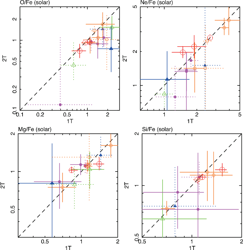
Figure 10: Comparison of abundance ratios of O/Fe, Ne/Fe, Mg/Fe, and Si/Fe with the 1T model and 2T model. Statement of meaning of the symbols is shown in Figure 7. The solid and dotted error bars show data, whose best fit model are 2T and 1T model, respectively. The dashed lines indicates the equal value between two models.

5.2 Comparison of metal abundances derived from AtomDB v1.3.1 and v2.0.1

The latest released AtomDB v2.0.1 include several measure update. The one of those is improvement in Fe L-shell strength predictions owing to incorporating new ionization balance data of Fe. We performed the spectral fit in the same way with the 1T and 2T APEC model for the ISM as in Section 4.1, but using AtomDB v1.3.1. The residuals of these fits have been listed as bottom panels in Figure 2 (and Appendix B). As shown in Figure 11, the two versions of AtomDB gave similar reduced ${\chi^{2}}$ with a some scatter. The derived temperatures with v2.0.1 are plotted against those with v1.3.1 in Figure 12. The temperatures derived with the v2.0.1 code are increased systematically by $\sim$ 10 %, except for NGC 1553. The derived temperatures reflect a change in the peak energy of the Fe-L line blend caused by the updates of the Fe-L atomic data. Since the emissivity of Ly$\alpha$ lines has a temperature dependence, the 10% difference in the derived ISM temperature between the two versions yields 10–20% under or overestimates of the O, Ne, Mg and Si abundances.

Figure 13 compare the O, Ne, Mg, Si and Fe abundances using the two versions of the AtomDB. We also calculated the weighted averages of the O, Ne, Mg, Si, and Fe abundances, and O/Fe, Ne/Fe, Mg/Fe, and Si/Fe ratios for the sample galaxies, and for the three temperature groups, and summarized in Table 5 and Figure 14. The new version of the AtomDB yielded almost the same values of Mg abundances with the old version, while it gave higher O abundances by 30–40% and higher Ne abundances by 50% and lower Si and Fe abundances by 10–30%. As a result, the O/Fe, Ne/Fe, and Mg/Fe ratios from the version 2.0.1 AtomDB are systematically higher than those from the old version by a factor of $\sim$ 1.6, 2.0, and 1.2, respectively, while the Si/Fe ratios did not change. The difference in the O/Fe ratio tends to be higher for galaxies with lower ISM temperatures, while no significant dependence on the ISM temperature is seen in the differences in the Ne/Fe, Mg/Fe and Si/Fe ratios.

In Loewenstein & Davis (2012), they have also investigated the differences of derived temperatures and metal abundances between AtomDB v1.3.1 and v2.0.1, although they fitted the simulated spectra, assumed single-temperature thermal plasma according to AtomDB v2.0.1. Our result, which is the relation of derived temperatures between v1.3.1 and v2.0.1, is good agreement with those of Loewenstein & Davis (2012). Furthermore, they compared the metal abundances, especially Fe, and concluded the derived Fe were overestimated using two-temperature models with the v1.3.1, which well reproduced the simulated spectra compared to fitting with one-temperature models. Our Fe abundances using v1.3.1, whose models are best fit model, are also systematically higher than those of v2.0.1.

Figure 11: Comparison of the reduced ${\chi^{2}}$ derived with AtomDB v1.3.1 and v2.0.1 in the energy range of 0.5–5 keV, 0.6–1 keV, and 1–1.3 keV in order from left to right panel.

Figure 12: Comparison of the ISM temperatures derived with AtomDB v1.3.1 and v2.0.1. Meanings of the symbols are the same as those in Figure 7. The dashed line indicates the equal value between two models.

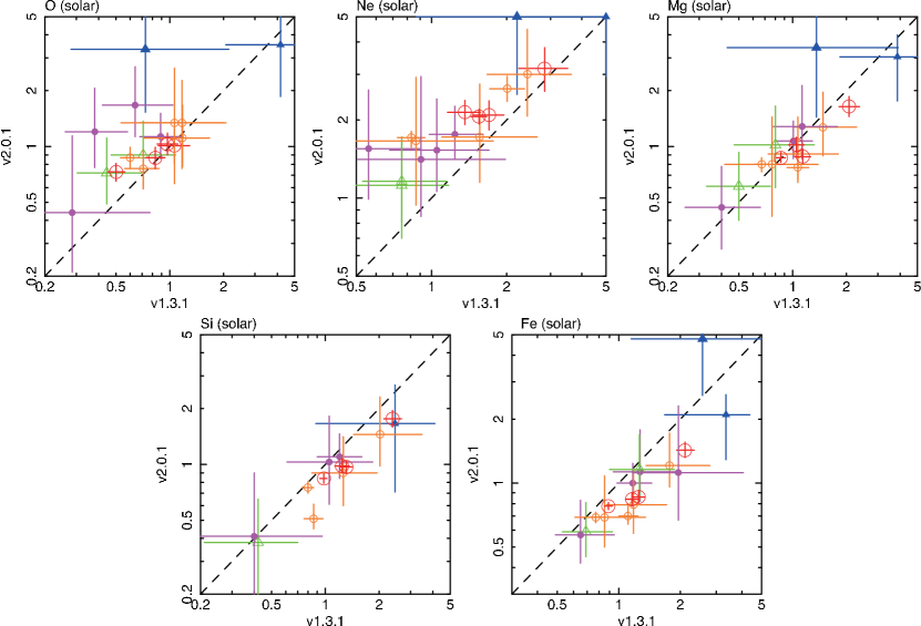
Figure 13: Comparison of abundances of O, Ne, Mg, Si, and Fe with v1.3.1 and v2.0.1 models. Meanings of the symbols are the same as those in Figure 7.

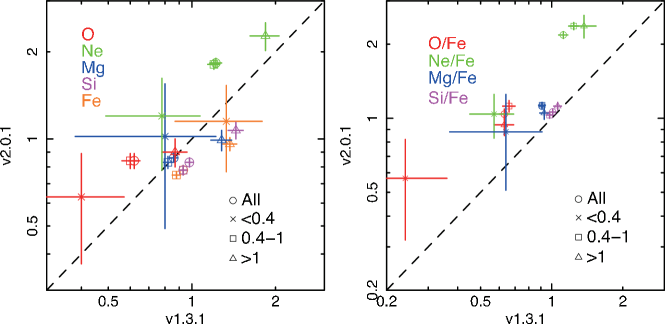
Figure 14: Comparison of the weighted averages of abundances (O, Ne, Mg, Si, and Fe; left) and abundance ratios (O/Fe, Ne/Fe, Mg/Fe, and Si/Fe; right) with AtomDB v1.3.1 and v2.0.1. The dashed line indicates the equal value between two models.

5.3 Residual structures at $\sim$ 0.8 keV

One of the major update in AtomDB v2.0.1 is the strength of emission in energy of 0.7–1.0 keV differ from those of v1.3.1, as shown in Figure 3 in Foster et al. (2012). The ratio of strong lines of Fe XVII at 15.0 Å and 17.1 Å  changed by several tens of % from AtomDB v1.3.1 to v2.0.1. This ratio expected from the latest version of other plasma code, SPEX, is located between the two versions of AtomDB at a given plasma temperature (de Plaa et al., 2012). This line ratio is often used to study the effect of resonant line scattering to constrain turbulence in the ISM (Xu et al., 2002; Hayashi et al., 2009; Werner et al., 2009; de Plaa et al., 2012). However, with AtomDB v1.3.1, there are residual structures around 0.8 keV in the spectra of NGC 1404 and NGC 720 with ISM temperatures of $\sim$ 0.6 keV observed with Suzaku (Matsushita et al., 2007; Tawara et al., 2008). Considering a poor spatial resolution of Suzaku and relatively compact ISM emission of these two galaxies, these residuals reflects the systematic uncertainties in the Fe-L atomic data, rather than the resonant line scattering.

As shown in Figure 2 and 23, using the v1.3.1 AtomDB, there are strong residual structure around 0.7–0.8 keV in the spectra of galaxies with ISM temperature of $\sim$ 0.6–0.8 keV. These structures mostly disappeared with v2.0.1. In Figure 11, the contribution of $\chi^{2}$ divided by the number of bins in the range of 0.6–1.0 keV using the v2.0.1 AtomDB are plotted against those of v1.3.1. The $\chi^{2}$ in this energy range drastically improved with the v2.0.1 AtomDB. Figure 15 shows the temperature dependence of ${\chi^{2}}$/bins in an energy range of 0.6–0.8 keV. The improvement of the $\chi^{2}$ are seen in galaxies with ISM temperatures of 0.3–0.8 keV. Since the energy of Ly$\alpha$ line of O VIII is close the residual structure at 0.7–0.8 keV, the measurements of O abundance can be affected by the revision of the atomic data at this energy range.

5.4 Residual structures at 1.2 keV

With the v2.0.1 AtomDB, the contribution of $\chi^{2}$ divided by the number of bins in the energy range of 1–1.3 keV of several galaxies increased significantly from the v1.3.1, although $\chi^{2}$/d.o.f for most of galaxies are consistent between the two version (Figure 11). As shown in Figure 15, some galaxies with the ISM temperatures higher than $\sim$0.6 keV show higher $\chi^{2}$ with v2.0.1, while the two versions gave similar $\chi^{2}$ values for the other galaxies with similar ISM temperatures. These high $\chi^{2}$ are caused by residual structures around 1.2 keV using the v2.0.1 AtomDB shown in the spectra of several galaxies such as NGC 1399 and NGC 4472. These 1.2 keV residuals have been observed in various kinds of objects (e.g., Yamaguchi et al., 2010; Loewenstein & Davis, 2012). Brickhouse et al. (2000) also interpreted this structure as a problem in the Fe-L atomic data. These residual structures should be attributed to suppression line around 1.2 keV in v2.0.1 than those of v1.3.1 from Figure 3 in Foster et al. (2012).

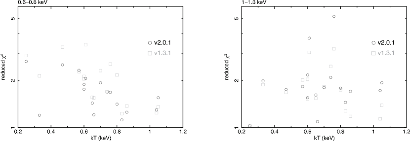
Figure 15: The contribution of $\chi^{2}$ divided by the number of bins in the range of 0.6–0.8 keV (left) and 1–1.3 keV (right) with AtomDB v1.3.1 (open squares) and v2.0.1 (open circles) in the energy range 0.6–0.8 (left) and 1–1.3 keV (right), plotted against the temperature of ISM with 1T model.

When we added a Gaussian model with the central energy of $\sim$1.23 keV to the spectral models in Section 4.1, the residual structure at $\sim$ 1.2 keV were disappeared. We plotted the equivalent widths of Gaussian lines from the two versions, v2.0.1 and v1.3.1, for galaxies with the residual structures against the ISM temperature and Fe abundance in Figure 16. The equivalent widths from v2.0.1 AtomDB are sometimes higher by an order of magnitude than those from v1.3.1. There are no clear dependence of the equivalent widths on the ISM temperature and Fe abundance. The 1.2 keV residuals should not affect on the O, Mg, Si, and Fe abundances very much because the derived values of these abundances with the Gaussian component did not change. In contrast, the Ne/Fe decreased. Therefore, the larger Ne abundances with AtomDB v2.0.1 than those with the old version can be caused by the change of the Fe-L line emission around 1.2 keV.

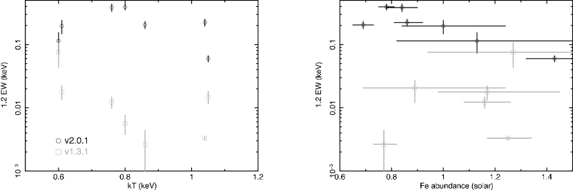
Figure 16: Equivalent widths of the Gaussian component at 1.23 keV are plotted against the temperatures of ISM (left panel) and Fe abundance (right panel). The black open circles and gray open squares are for AtomDB v2.0.1 and v1.3.1, respectively.

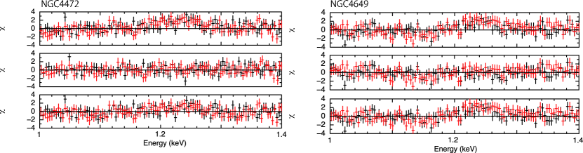
Figure 17: Residuals of fit the spectra of NGC 4472 (left) and NGC 4649 (right) using AtomDB v2.0.1 with the 1T or 2T model , those with the Gaussian component at 1.23 keV, those when the Ni abundance was allowed to vary in order from upper to bottom panel.

The residuals around 1.2 keV can affect on the derived Ni abundances, since the Ni-L lines peak around 1 keV. We fitted the spectra with the same model as Section 4.1 using the two version of AtomDB, but the Ni abundance was left free. However, the residual structures at 1.2 keV still remains as shown in Figure 17 (bottom panel). The derived Ni/Fe ratios are plotted in Figure 18. The Ni/Fe ratios become 1 – 8 in units of the solar ratio, with a very large scatter, and the difference in the Ni/Fe ratios between the two versions of AtomDB sometimes reaches a factor of 5. These large Ni/Fe ratios cannot be explained by any nucleosynthesis models for SN Ia.

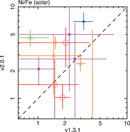
Figure 18: Comparison of the Ni/Fe ratios derived with AtomDB v1.3.1 and v2.0.1. The dashed line indicates the equal value between two models.

In summary, AtomDB v2.0.1 might have a problem in the Fe-L emission around 1.2 keV, and can affect on the abundance measurements of Ni and Ne abundances. However, the effect on the derived abundances of Fe, O, Mg, and Si are small.

5.5 Comparison with previous study

With XMM-Newton RGS, Xu et al. (2002) derived the metal abundances of O, Ne, Fe, and Mg in the ISM of an elliptical galaxy, NGC 4636, using an old version of APEC plasma code. With RGS, Werner et al. (2009) derived the metal abundances of N, O, Ne, and Fe in the ISM in 5 elliptical galaxies using SPEX plasma code (Kaastra et al., 1996). Since RGS has a superior energy resolution, the Ly$\alpha$ of O VIII lines were clearly detected with RGS. The derived O/Fe ratios by these papers are about 0.6–0.7 in unit of the solar ratio, using the solar abundance table by Lodders (2003). This value agrees well with the weighted average of the O/Fe ratio of $\sim 0.6$ in unit of the solar ratio of our sample galaxies derived with the 1T or 2T models for the ISM using AtomDB v1.3.1, although the new version of AtomDB gave much higher values of the O/Fe ratio, and absolute values sometimes show discrepancies.

We compare our results of AtomDB v1.3.1 for overlapping objects, NGC 720, NGC 1399, NGC 3923, NGC 4406, NGC 4472, NGC 4552, NGC 4636, and NGC 4649 with the previous measurements by Ji et al. (2009), which analyzed specific high-quality data of XMM-Newton EPIC and RGS and Chandra ACIS. The metal abundances by Ji et al. (2009) are converted using the solar abundance table by Lodders (2003). Our Mg/Fe and Si/Fe ratios agree well with those derived by Ji et al. (2009), while there are discrepancies in the absolute abundances and O/Fe ratios.

Loewenstein & Davis (2010) and Loewenstein & Davis (2012), analyzed the metal abundances in the ISM of NGC 4472 and NGC 4649 with Suzaku. The results of NGC 4649 are good agreement between their and our study, but their metal absolute abundances of NGC 4472 are systematically larger, although our Mg/Fe and Si/Fe ratios agree with those by Loewenstein & Davis (2010). The major differences for NGC 4472 are version of APEC code, regions for spectral accumulation, and treatment of background.

In summary, using the same version of plasma code, our measurements of the O/Fe, Mg/Fe, and Si/Fe ratios in the ISM mostly agree with previous measurements, while the absolute abundances sometimes have discrepancies. The abundance ratios are derived from the line ratios. In contrast, because the continuum level depends on the value of absolute abundance, the difference in the spectra with different absolute abundances is relatively small. Therefore, the systematic errors in the absolute abundances can be larger than the abundance ratios. Furthermore, the uncertainties in the emission from our Galaxy can cause a systematic error in the derived O abundance.

6 DISCUSSION

6.1 Metal abundance patterns and contributions from SNe

We successfully measured the abundance patterns of O, Mg, Si, and Fe in the ISM of 17 early-type galaxies, 13 ellipticals and 4 S0’s, with $L_{K}>L_{K*}$ and derived abundance ratios. Figure 19 shows the weighted averages of the O/Fe, Ne/Fe, Mg/Fe, and Si/Fe ratios of all of the sample galaxies derived with the multi-T fits using the APEC plasma code with AtomDB v2.0.1. The abundance ratios except for the Ne/Fe ratio agree very well with the solar ratios by Lodders (2003). The yields of core-collapse SN (hereafter SNcc) and SN Ia are also plotted in Figure 19. Here, the SNcc yields by Nomoto et al. (2006) refer to an average over the Salpeter initial mass function of stellar masses from 10 to 50 $M_{\odot}$, with a progenitor metallicity of $Z=0.02$. The SNe Ia yields were taken from the W7 mode by Iwamoto et al. (1999). The abundance ratios in the ISM are located between those of SNcc and SN Ia. The solar O/Fe, Mg/Fe, and Si/Fe ratios in the ISM indicate a same mixture of the two types of SN with the solar system. Considering that the O/Fe and Mg/Fe ratios of the SNcc yields expected from theoretical nucleosynthesis models by Nomoto et al. (2006) and observed abundance pattern of metal poor stars in our Galaxy (e.g., Edvardsson et al., 1993; Feltzing & Gustafsson, 1998; Bensby et al., 2003, 2004) are about three in units of the solar ratio, $\sim$70% and $\sim$30% of Fe are synthesized by SN Ia and SNcc, respectively,

The observed Ne/Fe ratios, about two in unit of the solar ratio, and the large Ni/Fe ratios with a significant scatter, cannot be explained by any mixture of the two types of SNe which can reproduce the solar O/Fe, Mg/Fe, and Si/Fe ratios. The Ne and Ni abundances may have intrinsic large systematic errors because their emission lines are hidden by prominent Fe-L lines.

The weighted averages of the abundance ratios of the hotter two temperature groups, 0.4–1 and $>1$ keV, agree very well with those for all the sample galaxies (Figure 19). On the other hand, mainly due to the low O/Fe and Ne/Fe abundances in the ISM of a S0 galaxy, NGC 4382, the lowest temperature group has smaller O/Fe and Ne/Fe ratios by a factor of two. To explain the lower O/Fe and Ne/Fe ratios in the ISM for the lowest temperature groups, we need a higher contribution of SNe Ia to Fe in the ISM.

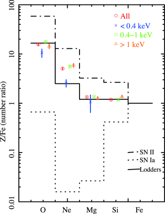
Figure 19: The weighted averages of the abundance ratios of O, Ne, Mg, and Si to Fe for the multi-T model with AtomDB v2.0.1. Red, blue, green, and orange data show for all the sample galaxies, temperature groups of $<$0.4 keV, 0.4–1 keV, and $>$1 keV, respectively. Solid, dot-dashed, and dotted lines represent the number ratios of metals to Fe for solar abundance (Lodders, 2003), for SNcc products (Nomoto et al., 2006), and for SN Ia ones (Iwamoto et al., 1999), respectively.

6.2 Comparison with optical measurements of stellar metallicity

Figure 20 shows the O, Mg, Si, and Fe abundances in the ISM derived from the multi-T model using the version 2.0.1 AtomDB, plotted against the central stellar velocity dispersion, $\sigma$. As found by optical observations for the stellar metallicity (e.g., Kuntschner et al., 2010), there is no environmental and morphological dependence on the O, Mg, and Si abundances. In Figure 20, we also plotted the best-fit relation of the stellar metallicity, $Z$, within $r_{\rm e}$ against $\sigma$ derived from optical spectroscopy by Kuntschner et al. (2010). Since O and other $\alpha$-elements mostly contribute the metallicity, we compared $Z$ with O, Mg, and Si abundances in the ISM (e.g., Tantalo et al., 1998). Among $\alpha$ elements, Mg abundances in the ISM have smallest systematic error in our analysis and are mainly used to derive metal abundance $Z$ in optical observations. Except for a few galaxies, the derived Mg and Si abundances in the ISM mostly agree with the $Z$–$\sigma$ relation by Kuntschner et al. (2010). Although Si are synthesized by both SN Ia and SNcc, the solar abundance pattern indicates that most of Si come from SNcc and therefore, it is reasonable to have the same $Z$–$\sigma$ relation with Mg. Two S0 galaxies in the field or small groups show significantly higher Mg abundances than the other galaxies. However, the systematic differences due to different versions of APEC models and temperature modelling of the ISM in these galaxies are also larger than the other ones.

In Kuntschner et al. (2010), they adopted the solar abundance table by Grevesse & Sauval (1998), and the other for the abundance pattern of CN-strong stars Cannon et al. (1998). In optical observations, the metallicity is derived from the combination of the strength of Mg and Fe absorption lines. However, the solar O abundance derived from solar photospheric lines has been changed by several tens of %, considering three-dimensional hydro-static model atmospheres and non-local thermodynamic equilibrium (e.g., Asplund et al., 2005). In this paper, we use the new solar abundance table by Lodders (2003), adopting this O abundance. Therefore, in Figure 20, we plotted the same $Z$–$\sigma$ relation by Kuntschner et al. (2010) and that converted to the table by Lodders (2003) considering the difference in the solar abundance tables. The O abundances in the ISM agree well with the original $Z$–$\sigma$ relation, but systematically offset from the converted one. However, the slope of the O abundance–$\sigma$ relation agrees very well with the optical $Z$–$\sigma$ relation. When we compared the absolute metal abundances between optical and X-ray observations, there are systematic errors coming from the differences of solar abundance tables, the ways of the observations, and uncertainties of emission models. The trends of all elements are agree with the $Z$–$\sigma$ relation.

Optical observations indicate that negative radial gradients of stellar metallicity in elliptical galaxies are common. Assuming that the same metallicity gradient continues beyond $r_{\rm e}$, the average stellar metallicity of entire galaxy is similar to that at $r_{\rm e}$ (Kobayashi & Arimoto, 1999). The differences in the stellar metallicity within $r_{\rm e}$ and at $r_{\rm e}$ of elliptical galaxies derived by the optical observations are typically around 0.1 dex, or a factor of 1.2–1.3 (Kuntschner et al., 2010). Our measurements of the ISM abundances indicate that the average stellar metallicity of entire galaxies with $\sigma>200\rm{kms^{-1}}$ are close to the solar metallicity, and the metallicity-mass relation is consistent with that of the stellar relation for the $r_{\rm e}$ region. Although we are comparing abundances in two distinct media, stars and ISM, which could have very different histories, and different systematic errors, the agreement of the metallicity between the hot ISM and stars indicates relatively small systematic errors in the measurements with these optical and X-ray observations.

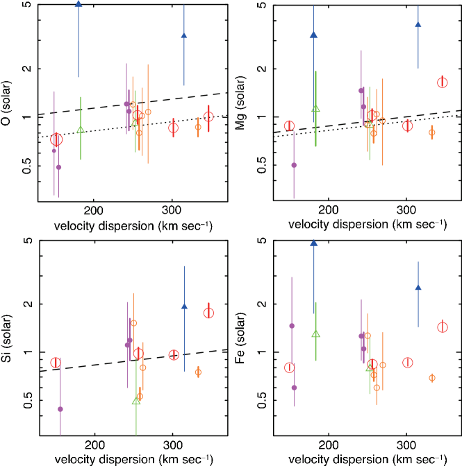
Figure 20: The abundances of O, Mg, Si, and Fe in the ISM derived from the multi-T model fits with AtomDB v2.0.1 are plotted against the central stellar velocity dispersion by Prugniel & Simien (1996). Meanings of the symbols are the same as those in Figure 7. The dashed and dotted lines show the $Z$–$\sigma$ relation for a $r_{\rm e}$ aperture derived from optical spectroscopy by Kuntschner et al. (2010) and that converted considering the difference in the solar abundance tables, respectively.

6.3 Comparison with optical measurements of stellar $\alpha$/Fe ratios

In Figure 21, the O/Fe, Mg/Fe, and Si/Fe ratios in the ISM are plotted against $\sigma$. We note that the Mg/Fe ratios have smallest systematic differences between the two versions of plasma codes and among the different modeling of the temperature structure for the ISM. Again, there is no systematic difference in the O/Fe, Mg/Fe, and Si/Fe ratios between the ellipticals and S0 galaxies, or between those in the field or small groups and in clusters. The O/Fe and Mg/Fe ratios of the two S0 galaxies with higher O and Mg abundances are consistent with those of the others. The dot-dashed lines in these plots correspond to the best-fit relation between [$\alpha/\rm{Fe}$] within $r_{\rm e}$ and $\sigma$ derived from optical spectroscopy by Kuntschner et al. (2010). The O/Fe, Mg/Fe, and Si/Fe ratios in the ISM are systematically smaller by a factor of two than the relation for the stellar metallicity. Therefore, we need additional SN Ia enrichment in the ISM to account for both of the X-ray and optical observations of early-type galaxies.

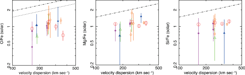
Figure 21: The abundance ratios of O/Fe, Mg/Fe, and Si/Fe in the ISM derived from the multi-T model fits with AtomDB v2.0.1 are plotted against central stellar velocity dispersion by Prugniel & Simien (1996). Meanings of the symbols are the same as those in Figure 7. The dot-dashed and dotted lines show the [$\alpha$/Fe]–$\sigma$ relation for a $r_{\rm e}$ aperture derived from optical spectroscopy by Kuntschner et al. (2010) and that converted considering the difference in the solar abundance tables, respectively.

A longer star-formation time scale yields more SNe Ia products in stars, and therefore, the difference in the $\alpha$/Fe ratio in stars can constrain the star formation histories. As shown in Figure 21, the optical observations indicate that massive galaxies show higher O/Fe, Mg/Fe, and Si/Fe ratios and therefore shorter star formation time scales. Considering typical timescale for SN Ia from star formation (Kobayashi & Nomoto, 2009), duration of major star formation should be shorter than a few Gyr. Although we cannot distinguish the SNe Ia yields in the ISM from present SNe Ia and those trapped in stars and the errors in the O/Fe, Mg/Fe, and Si/Fe ratios in the ISM of galaxies with small $\sigma$ are relatively large, our measurements are consistent with the [$\alpha$/Fe]–$\sigma$ relation derived from the optical spectroscopy by Kuntschner et al. (2010) for a $r_{\rm e}$ aperture, assuming an additional enrichment of the Fe abundance of $\sim$ 0.5 solar from the present SN Ia. As described in Section 6.2, although both SN Ia an SNcc produce Si, the Si/Fe ratios have similar trend compared to those of O/Fe and Mg/Fe ratios. Since the Si/Fe ratio is solar abundance, Si in the ISM should come from by SNcc.

There are no difference in the abundances and their ratios in the ISM between the cluster galaxies and those in the field or small groups. The similarity of the abundances in the ISM indicate that major star formation history are similar. There are also no dependence in the ISM abundance patterns between elliptical and S0 galaxies. Then, major star formation histories of these galaxies may be similar with those of ellipticals, although a possibility of spiral galaxies changed into S0 galaxies is discussed based on the fractional evolution of S0 and spiral galaxies in clusters (e.g., Dressler et al., 1997; Kodama et al., 2004; Poggianti et al., 2009). The two S0 galaxies in clusters in our sample, NGC 1316 and NGC 4382 have indications of experiences of recent major mergers (e.g., Goudfrooij et al., 2001; Sansom et al., 2006). NGC 4382 has smaller O/Fe and Ne/Fe ratios in the ISM by a factor of two than the other galaxies. Considering that the reported present SN Ia rate in S0 and elliptical galaxies are consistent with each other (e.g., Mannucci et al., 2008), Fe abundances from recent SN Ia should be similar between the two types of galaxies. Consequently, the SN Ia products included in stars of NGC 4382 are larger than those of other early-type galaxies. If this galaxy is formed with a merging of massive spiral galaxies, the stars contains significant amount of SN Ia yields as in our Galaxy,

6.4 Present Fe enrichment by SN Ia

The Fe abundance synthesized by present SNe Ia in an early-type galaxy is calculated by $M^{\rm Fe}_{\rm SN}\theta_{\rm SN}/\alpha_{*}z^{\rm Fe}_{\rm solar}$ (see Matsushita et al. (2003) for details). Here, $M^{\rm Fe}_{\rm SN}$ is the Fe mass synthesized by one SN Ia, $\theta_{\rm SN}$ is the SN Ia rate, $\alpha_{*}$ is the stellar mass loss rate, and $z^{\rm Fe}_{\rm solar}$ is the solar Fe mass fraction. We used the mass-loss rate from Ciotti et al. (1991), which is approximated by $1.5\times 10^{-11}L_{\rm B}t^{-1.3}_{15}M_{\odot}\rm{yr}^{-1}$, where $t_{15}$ is the age in units of 15 Gyr and $L_{\rm B}$ is the B-band luminosity. $M_{\rm Fe}$ produced by one SN Ia explosion is likely to be $\sim 0.6M_{\odot}$ (Iwamoto et al., 1999). Since there are no significant difference of SN Ia rate between elliptical and S0 galaxies, we adopted 0.1–0.5 $\rm{SN~{}Ia}/100\rm{yr}/$ $10^{10}L_{\rm B}$ as the optically observed SN Ia rate (e.g., Mannucci et al., 2008; Blanc et al., 2004; Hardin et al., 2000; Cappellaro et al., 1997). We used the solar Fe mass fraction 0.0012 from Lodders (2003). The estimated stellar age assuming a single-stellar population for massive early-type galaxies are typically older than 10 Gyr (e.g., Thomas et al., 2005; Kuntschner et al., 2010). The resultant Fe abundance is 2.8-13.9 solar assuming the stellar age of 13 Gyr. Assuming a stellar age of 10 Gyr, the mass-loss rate increase by 1.4 times, and the contribution of SN Ia to Fe abundance decreases by 0.7 times, and the expected Fe abundance from SN Ia becomes 2.0–9.7 solar.

Since the weighted average of the Fe abundances in the ISM is 0.8 solar, the contribution from SN Ia should be about 0.5 solar ($\sim$70% of Fe abundance synthesized by SN Ia from Section 6.1), which is a sum of those in stars and present SN Ia. On the other hands, if an average of the stellar metallicity and $[\alpha$/Fe] ratio over entire galaxies are close to the relations of $Z$–$\sigma$ and [$\alpha$/Fe]–$\sigma$, respectively, derived by Kuntschner et al. (2010), we need a Fe abundances of about $\sim$ 0.5 solar from present SNe Ia (Figure 21). Therefore, if all the ejecta of SNe Ia have been completely mixed into the ISM, the present SN Ia rate to account for the observed Fe abundance in the ISM is significantly smaller than those measured by optical SN Ia observations. With estimated Fe abundance from present SNe Ia, the calculated SN Ia rate is $\sim$0.02.

If some part of SN Ia ejecta can escape the ISM before fully mixed in to the ISM (Matsushita et al., 2000; Tang & Wang, 2010; Loewenstein & Davis, 2012), the Fe abundance can be lower. Tang & Wang (2010) simulated the evolution of SN Ia ejecta in the galaxy-wide hot gas out-flows. They found that SN Ia ejecta producing little X-ray emission and driven by its large buoyancy, can quickly get higher outward velocity. Since this ejecta slowly diluted and cooled, and as a result, they expect that the emission-weighted Fe abundance of central few kpc becomes significantly smaller. However, no significant radial gradients in the Mg/Fe ratios are detected with Suzaku, XMM and Chandra observations (Ji et al., 2009; Hayashi et al., 2009; Loewenstein & Davis, 2012). Furthermore, the X-ray luminous objects surrounded by larger-scale potentials (large open circles in Figure 20 and 21), and NGC 1404, which has a compact ISM emission due to ram-pressure stripping (Machacek et al., 2005), have similar values of O/Fe and Mg/Fe ratios as well as the O, Mg, and Fe abundances with the other galaxies. Since the ISM mass within 4 $r_{\rm e}$ in these X-ray luminous galaxies are several times larger than those in the X-ray fainter galaxies, the accumulation time scale for the ISM should be different. Therefore, the idea of the partial mixing of the SN Ia ejecta into the ISM also has an difficulty to explain the observed abundance pattern in the ISM.

The ICM in clusters of galaxies contains a large amount of metals. The observed abundance pattern of the ICM indicates that most of Fe in the ICM were synthesized by SN Ia (e.g. Sato et al., 2007, 2009; Matsushita et al., 2012). Suzaku enabled us to measure the Fe mass in the ICM out to the virial radius (Sato et al., 2012; Matsushita et al., 2012). The observed ratios of Fe mass in the ICM to the total light from galaxies, iron-mass-to-light ratio (IMLR), out the virial radius of Hydra A and the Perseus clusters reach $\sim 10^{-2}M_{\odot}/L_{K,\odot}$. However, accumulating the observed SN Ia rate by optical observations over the Hubble time, 13.7 Gyr, the expected IMLR from the SN Ia becomes (2–5)$\times 10^{-4}M_{\odot}/L_{K,\odot}$. Adopting the SN Ia rate indicated from X-ray measurements of the Fe abundance in the ISM assuming that SN Ia ejecta well mixed into the ISM, the expected IMLR from the SN Ia becomes even smaller, $\sim 10^{-4}M_{\odot}/L_{K,\odot}$. These results indicate that the lifetimes of most of SN Ia are much shorter than the Hubble time, and the SN Ia rate in cluster galaxies was much higher in the past.

7 CONCLUSION

We performed X-ray spectral analysis of 17 early-type galaxies, 13 ellipticals and 4 S0s, with Suzaku. The spectra extracted from 4 $r_{\rm e}$ have been produced with 1T or 2T thermal plasma model and the multi-T model for the ISM. We successfully measured the metal abundance patterns O, Mg, Si, and Fe of the ISM and derived abundance ratios. The weighted averages of the O, Mg, Si, and Fe abundances of all the sample galaxies derived from the multi-temperature model fits are 0.83 $\pm$ 0.04, 0.93$\pm$0.03, 0.80 $\pm$ 0.02, and 0.80$\pm$0.02 solar, respectively, in solar units according to the solar abundance table by Lodders (2003). The abundance ratios of O/Fe, Mg/Fe, and Si/Fe are close to the solar ratio. The derived values of Ne and Ni abundances may have larger systematic uncertainties because their emission lines are hidden by the Fe-L lines. The O and Mg abundances in the ISM within 4 $r_{\rm e}$ agree well with the stellar metallicity derived by the optical observations for $r_{\rm e}$ apertures. This agreement indicates relatively small systematic errors in the measurements with these optical and X-ray observations. The solar O/Fe and Mg/Fe ratios in the ISM indicate additional contribution from present SN Ia. There is no systematic differences between galaxies in clusters and field or small groups or between elliptical and S0 galaxies. Therefore, major star formation history should be similar among these objects. The Fe abundance in the ISM is significantly smaller than the expected value derived from optical observations, indicates a low present SN Ia rate.

Appendix A TREATMENT AND RESULTS OF CONTAMINANT ON XIS

The quantum efficiency of XIS in the low energy range has been decreasing owing to OBF (see detail in The Suzaku Technical Description). In usual, we make a ARF file using calibration file of contaminant, which have information of thickness of contaminant at the center region in chronological order. Furthermore, they reproduce the space distribution of contaminant with a simple function of position. It is very difficult, however, to completely predict the distribution of contaminant material because of time-varying composition, thickness, and configuration. Especially, in recent observations, outer region of detector, and XIS0/3, some discrepancies between data and model under $\sim$0.6 keV are known even if using calibration files.

As mentioned in Section 3, we have fit the spectra of all sample galaxy with ARF file including CALDB file contaminant and figured out there are still discrepancies for some galaxies. We attributed these discrepancies to difficulty to reproduce the contaminant profile about for the galaxies observed since the beginning of 2008. On the other hands, about for NGC 4472 and NGC 4649 observed in 2006, systematic error of contaminant estimation becomes pronounced because of very bright galaxies. We have performed spectral fit of data observed since the beginning of 2008 with ARF files without including the effect of the contaminant. Table 6 shows how we set calibration file or not, as making ARF files. When we fit the spectra with “varabs” model, the parameter of C in “varabs” were set to free. Meanwhile, we set O, corresponding to the ratios of C/O is values from Table 7 in units of solar ratio. The values of Table 7 are the ratios of C/O at the center of each detector from calibration files, ae_xi0 (or 1 or 2 or 3)_contami_20091201.fits. In the Table 8, we summarized the derived C vales of varabs model with 1T or 2T fit. The derived values of C is about 2/3 and 1/2 times of those values of calibration files for 4r_e and background region, respectively.

We checked whether the results of fitting with ARF files without including the effect of contaminant are consistent to those with calibration files of contaminant, whose name are ae_xi0 (or 1 or 2 or 3)_contami_20091201.fits. Then, NGC 1316 which observed in 2006 have been reanalyzed, using ARFs without the effect of contaminant. We fitted the spectra of the 4r_e and background regions simultaneously with same model in Section 4.1. All derived parameters are consistent between the two fits. We also summarized the ratios of metals in Figure 22, these are also in good agreement.

Table 6: Applied Calibration file of contaminant

Galaxy	BGD			4r${\rm e}$
	XIS0	XIS1	XIS3	XIS0	XIS1	XIS3
NGC 1332	no	20091201	no	20091201	20091201	20091201
NGC 2300	no	20091201	no	20091201	20091201	20091201
NGC 4125	no	20091201	no	no	20091201	no
NGC 4382	no	20091201	20091201	20091201	20091201	20091201
NGC 4406	no	no	no	no	no	no
NGC 4472	no	no	no	no	no	no
NGC 4649	no	no	no	no	no	no
NGC 4697	no	20091201	no	no	20091201	20091201
NGC 5846	no	20091201	20091201	20091201	20091201	20091201

Table 7: The set ratios of C to O in varabs model.

Galaxy	BGD			4r${\rm e}$
	XIS0	XIS1	XIS3	XIS0	XIS1	XIS3
NGC 1332	7.27	$\cdots$	7.27	$\cdots$	$\cdots$	$\cdots$
NGC 2300	7.31	$\cdots$	7.31	$\cdots$	$\cdots$	$\cdots$
NGC 4125	7.33	$\cdots$	7.34	7.33	$\cdots$	7.34
NGC 4382	7.61	$\cdots$	$\cdots$	$\cdots$	$\cdots$	$\cdots$
NGC 4406	7.37	7.08	7.10	7.37	7.08	7.10
NGC 4472	9.63	9.64	9.64	9.63	9.64	9.64
NGC 4649	9.45	9.35	9.36	9.45	9.35	9.36
NGC 4697	7.27	$\cdots$	7.27	7.27	$\cdots$	$\cdots$
NGC 5846	7.57	$\cdots$	$\cdots$	$\cdots$	$\cdots$	$\cdots$

Table 8: The C column densities (10${}^{22}\rm cm^{-2}$) in varabs model derived from the 1T or 2T model fits using APEC plasma code v2.0.1.

Galaxy	BGD			4r${\rm e}$
	XIS0	XIS1	XIS3	XIS0	XIS1	XIS3
NGC 1332	1.05${}^{+0.24}_{-0.23}$	$\cdots$	1.18${}^{+0.24}_{-0.23}$	$\cdots$	$\cdots$	$\cdots$
NGC 2300	1.58${}^{+0.19}_{-0.18}$	$\cdots$	1.53${}^{+0.18}_{-0.17}$	$\cdots$	$\cdots$	$\cdots$
NGC 4125	1.13${}^{+0.22}_{-0.21}$	$\cdots$	1.42${}^{+0.23}_{-0.22}$	1.69${}^{+0.18}_{-0.18}$	$\cdots$	1.60${}^{+0.18}_{-0.18}$
NGC 4382	0.86${}^{+0.17}_{-0.17}$	$\cdots$	$\cdots$	$\cdots$	$\cdots$	$\cdots$
NGC 4406	1.78${}^{+0.12}_{-0.12}$	1.72${}^{+0.10}_{-0.10}$	2.24${}^{+0.12}_{-0.12}$	2.18${}^{+0.09}_{-0.08}$	1.23${}^{+0.21}_{-0.18}$	2.26${}^{+0.08}_{-0.08}$
NGC 4472	0.48${}^{+0.13}_{-0.13}$	0.86${}^{+0.11}_{-0.10}$	1.60${}^{+0.08}_{-0.08}$	1.38${}^{+0.08}_{-0.08}$	1.29${}^{+0.26}_{-0.22}$	2.39${}^{+0.08}_{-0.08}$
NGC 4649	1.15${}^{+0.18}_{-0.14}$	1.52${}^{+0.17}_{-0.13}$	2.14${}^{+0.19}_{-0.15}$	1.77${}^{+0.09}_{-0.07}$	2.17${}^{+0.07}_{-0.05}$	2.53${}^{+0.09}_{-0.07}$
NGC 4697	1.21${}^{+0.15}_{-0.15}$	$\cdots$	1.45${}^{+0.14}_{-0.13}$	1.84${}^{+0.16}_{-0.16}$	$\cdots$	$\cdots$
NGC 5846	1.17${}^{+0.07}_{-0.07}$	$\cdots$	$\cdots$	$\cdots$	$\cdots$	$\cdots$

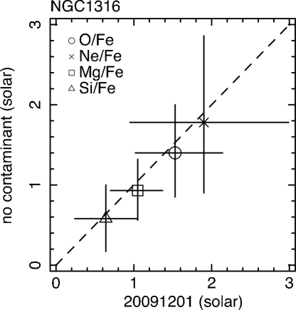
Figure 22: Comparison of abundance ratios (O/Fe, Ne/Fe, Mg/Fe, and Si/Fe) with varabs model and ARF file using calibration file ae_xi0 (or 1 or 2 or 3)_contami_20091201.fits. The dashed line indicate the equal value between two models.

Appendix B FIT SPECTRA IN SECTION 4.1

In this section, we summarized the background parameters and spectra in Section 4.1. The caption of figures are same as Figure 2.

Table 9: Best fit parameters from background region fit in the Section 4.1.1. Metal abundances of “vapec” model of NGC 1399 and NGC 4636 are summarized in Table 10.

Galaxy	kTGalactic	kTGalactic	kTETE	Abundance	${\chi^{2}}$/d.o.f.
	(keV)	(keV)	(keV)	(solar)
NGC 720	0.09${}^{+0.03}_{-0.06}$	0.20${}^{+0.06}_{-0.02}$	0.64${}^{+0.09}_{-0.03}$	0.19${}^{+0.11}_{-0.06}$	284/228
NGC 1316	0.09 (fix)	0.22${}^{+0.05}_{-0.02}$	0.91${}^{+0.04}_{-0.04}$	0.3 (fix)	169/174
NGC 1332	0.07${}^{+0.02}_{-0.01}$	0.30${}^{+0.04}_{-0.04}$	$\cdots$	$\cdots$	193/173
NGC 1399	$\cdots$	$\cdots$	1.67${}^{+0.16}_{-0.04}$	$\cdots$	698/460
	$\cdots$	$\cdots$	1.12${}^{+0.12}_{-0.04}$	$\cdots$	$\cdots$
NGC 1553	0.07 (fix)	0.19 (fix)	0.75${}^{+0.05}_{-0.05}$	0.22${}^{+0.30}_{-0.09}$	203/175
NGC 2300	0.13${}^{+0.03}_{-0.03}$	$\cdots$	0.93${}^{+0.02}_{-0.02}$	0.15${}^{+0.18}_{-0.03}$	263/202
NGC 3923	0.11 (fix)	0.19 (fix)	0.70${}^{+0.03}_{-0.03}$	0.55${}^{+2.92}_{-0.27}$	307/230
NGC 4125	0.07${}^{+0.02}_{-0.01}$	0.30${}^{+0.02}_{-0.02}$	$\cdots$	$\cdots$	211/173
NGC 4382	0.10${}^{+0.02}_{-0.01}$	0.28${}^{+0.02}_{-0.02}$	$\cdots$	$\cdots$	197/174
NGC 4406	0.10 (fix)	0.23 (fix)	0.97${}^{+0.02}_{-0.03}$	0.83${}^{+0.52}_{-0.23}$	385/349
	$\cdots$	$\cdots$	1.52${}^{+0.15}_{-0.13}$	0.3 (fix)	$\cdots$
NGC 4472	0.11${}^{+0.02}_{-0.02}$	$\cdots$	1.08${}^{+0.17}_{-0.03}$	0.73${}^{+0.13}_{-0.09}$	380/349
	$\cdots$	$\cdots$	1.74${}^{+0.49}_{-0.12}$	linked	$\cdots$
NGC 4552	0.13${}^{+0.02}_{-0.04}$	$\cdots$	2.00${}^{+0.49}_{-0.32}$	0.3 (fix)	271/246
NGC 4636	0.13 (fix)	0.21 (fix)	0.89${}^{+0.01}_{-0.01}$	$\cdots$	647/461
NGC 4649	0.07 (fix)	0.17 (fix)	0.98${}^{+0.02}_{-0.02}$	0.12${}^{+0.02}_{-0.01}$	490/351
NGC 4697	0.11${}^{+0.01}_{-0.01}$	0.27${}^{+0.01}_{-0.02}$	$\cdots$	$\cdots$	202/173
NGC 5846	0.12 (fix)	0.22${}^{+0.02}_{-0.01}$	0.67${}^{+0.09}_{-0.02}$	0.46${}^{+0.06}_{-0.05}$	267/201
	$\cdots$	$\cdots$	1.17${}^{+0.04}_{-0.03}$	linked	$\cdots$

Table 10: The O, Ne, Mg, Si, S, and Fe abundances in the ISM of NGC 1399 and NGC 4636 derived from background region fit in the Section 4.1.1.

Galaxy	O	Ne	Mg	Si	S	Fe
	(solar)	(solar)	(solar)	(solar)	(solar)	(solar)
NGC 1399	0.44$\pm{0.10}$	2.10${}^{+0.31}_{-0.30}$	0.78$\pm{0.08}$	0.82$\pm{0.05}$	0.82$\pm{0.07}$	0.77$\pm{0.04}$
NGC 4636	0.60${}^{+0.21}_{-0.20}$	1.22${}^{+0.19}_{-0.18}$	0.51${}^{+0.08}_{-0.07}$	0.38${}^{+0.06}_{-0.05}$	=Si	0.36${}^{+0.03}_{-0.03}$

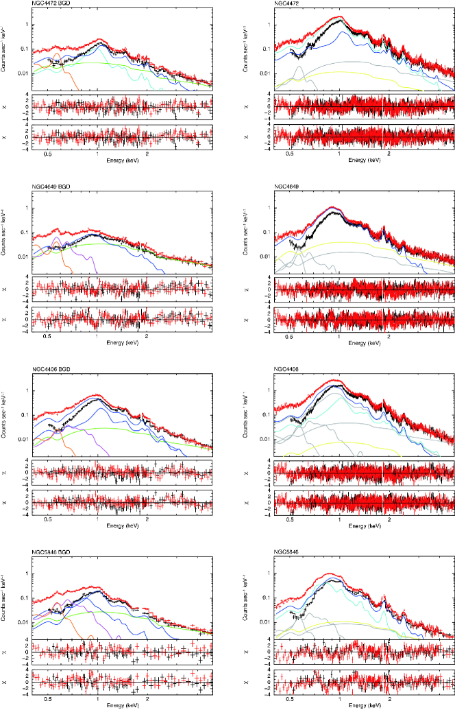
Figure 23: The same as Figure 2 for the galaxies are not shown in the Figure 2.

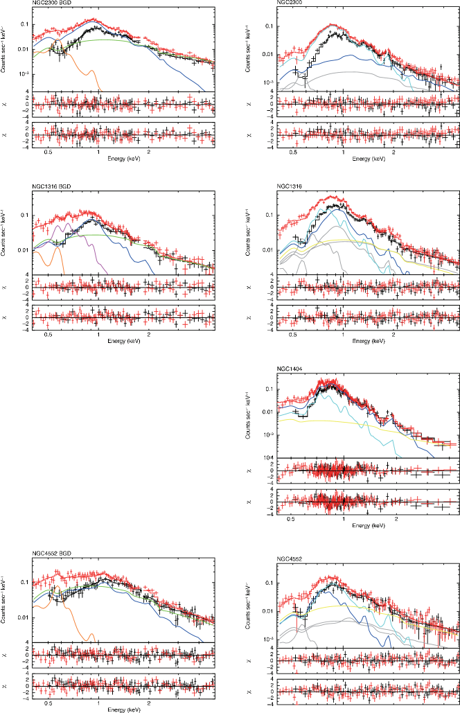
Figure 23: Continued.

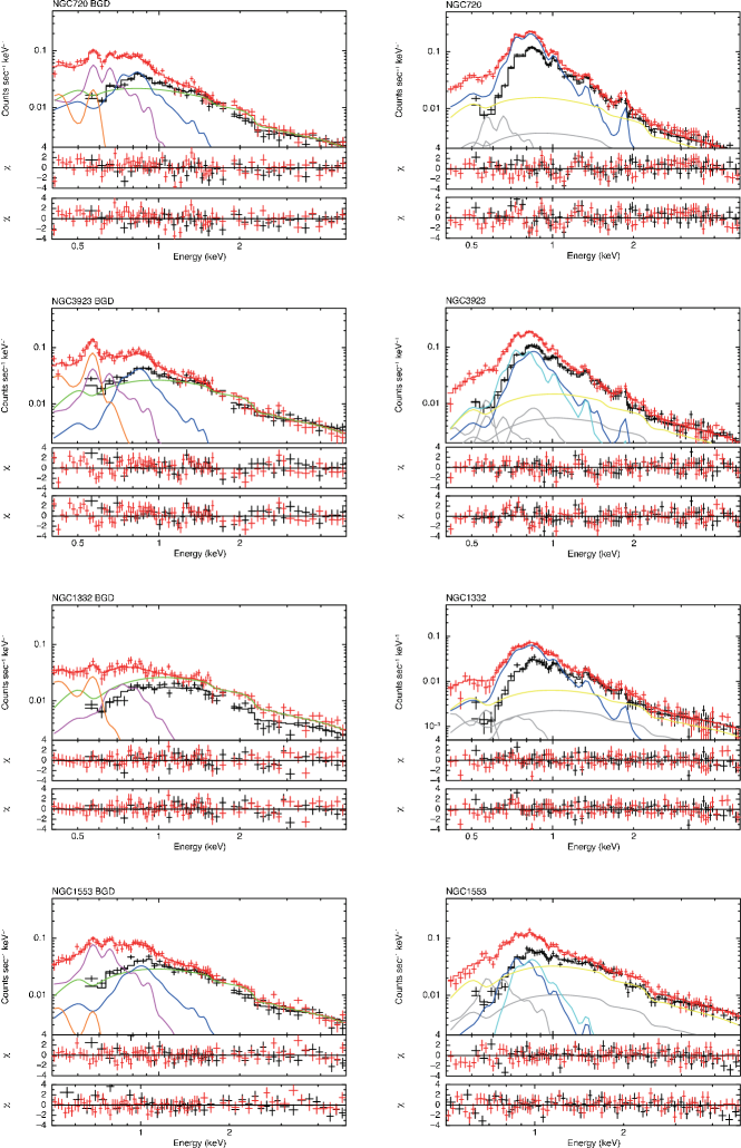
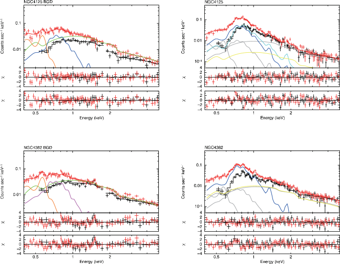
Figure 23: Continued.

Figure 23: Continued.

References

- Arimoto et al. (1997) Arimoto, N., Matsushita, K., Ishimaru, Y., Ohashi, T., & Renzini, A. 1997, ApJ, 477, 128
- Asplund et al. (2005) Asplund, M., Grevesse, N., & Sauval, A. J. 2005, in Astronomical Society of the Pacific Conference Series, Vol. 336, Cosmic Abundances as Records of Stellar Evolution and Nucleosynthesis, ed. T. G. Barnes, III & F. N. Bash, 25
- Awaki et al. (1994) Awaki, H., Mushotzky, R., Tsuru, T., et al. 1994, PASJ, 46, L65
- Bedregal et al. (2008) Bedregal, A. G., Aragón-Salamanca, A., Merrifield, M. R., & Cardiel, N. 2008, MNRAS, 387, 660
- Bensby et al. (2003) Bensby, T., Feltzing, S., & Lundström, I. 2003, A&A, 410, 527
- Bensby et al. (2004) —. 2004, A&A, 415, 155
- Blanc et al. (2004) Blanc, G., Afonso, C., Alard, C., et al. 2004, A&A, 423, 881
- Boroson et al. (2011) Boroson, B., Kim, D.-W., & Fabbiano, G. 2011, ApJ, 729, 12
- Brickhouse et al. (2000) Brickhouse, N. S., Dupree, A. K., Edgar, R. J., et al. 2000, ApJ, 530, 387
- Buote & Fabian (1998) Buote, D. A., & Fabian, A. C. 1998, MNRAS, 296, 977
- Cannon et al. (1998) Cannon, R. D., Croke, B. F. W., Bell, R. A., Hesser, J. E., & Stathakis, R. A. 1998, MNRAS, 298, 601
- Cappellaro et al. (1997) Cappellaro, E., Turatto, M., Tsvetkov, D. Y., et al. 1997, A&A, 322, 431
- Ciotti et al. (1991) Ciotti, L., D’Ercole, A., Pellegrini, S., & Renzini, A. 1991, ApJ, 376, 380
- Davis et al. (1996) Davis, D. S., Mulchaey, J. S., Mushotzky, R. F., & Burstein, D. 1996, ApJ, 460, 601
- de Plaa et al. (2012) de Plaa, J., Zhuravleva, I., Werner, N., et al. 2012, A&A, 539, A34
- de Vaucouleurs et al. (1991) de Vaucouleurs, G., de Vaucouleurs, A., Corwin, Jr., H. G., et al. 1991, Third Reference Catalogue of Bright Galaxies. Volume I: Explanations and references. Volume II: Data for galaxies between 0h and 12h. Volume III: Data for galaxies between 12h and 24h.
- Dickey & Lockman (1990) Dickey, J. M., & Lockman, F. J. 1990, ARA&A, 28, 215
- Dressler et al. (1997) Dressler, A., Oemler, Jr., A., Couch, W. J., et al. 1997, ApJ, 490, 577
- Edvardsson et al. (1993) Edvardsson, B., Andersen, J., Gustafsson, B., et al. 1993, A&A, 275, 101
- Feltzing & Gustafsson (1998) Feltzing, S., & Gustafsson, B. 1998, A&AS, 129, 237
- Foster et al. (2012) Foster, A. R., Ji, L., Smith, R. K., & Brickhouse, N. S. 2012, ApJ, 756, 128
- Goudfrooij et al. (2001) Goudfrooij, P., Alonso, M. V., Maraston, C., & Minniti, D. 2001, MNRAS, 328, 237
- Grevesse & Sauval (1998) Grevesse, N., & Sauval, A. J. 1998, Space Sci. Rev., 85, 161
- Hardin et al. (2000) Hardin, D., Afonso, C., Alard, C., et al. 2000, A&A, 362, 419
- Hayashi et al. (2009) Hayashi, K., Fukazawa, Y., Tozuka, M., et al. 2009, PASJ, 61, 1185
- Humphrey & Buote (2006) Humphrey, P. J., & Buote, D. A. 2006, ApJ, 639, 136
- Ishisaki et al. (2007) Ishisaki, Y., Maeda, Y., Fujimoto, R., et al. 2007, PASJ, 59, 113
- Iwamoto et al. (1999) Iwamoto, K., Brachwitz, F., Nomoto, K., et al. 1999, ApJS, 125, 439
- Ji et al. (2009) Ji, J., Irwin, J. A., Athey, A., Bregman, J. N., & Lloyd-Davies, E. J. 2009, ApJ, 696, 2252
- Kaastra et al. (1996) Kaastra, J. S., Mewe, R., & Nieuwenhuijzen, H. 1996, in UV and X-ray Spectroscopy of Astrophysical and Laboratory Plasmas, ed. K. Yamashita & T. Watanabe, 411–414
- Kobayashi & Arimoto (1999) Kobayashi, C., & Arimoto, N. 1999, ApJ, 527, 573
- Kobayashi & Nomoto (2009) Kobayashi, C., & Nomoto, K. 2009, ApJ, 707, 1466
- Kodama et al. (2004) Kodama, T., Yamada, T., Akiyama, M., et al. 2004, MNRAS, 350, 1005
- Konami et al. (2010) Konami, S., Matsushita, K., Nagino, R., et al. 2010, PASJ, 62, 1435
- Koyama et al. (2007) Koyama, K., Tsunemi, H., Dotani, T., et al. 2007, PASJ, 59, 23
- Kuntschner et al. (2010) Kuntschner, H., Emsellem, E., Bacon, R., et al. 2010, MNRAS, 408, 97
- Kushino et al. (2002) Kushino, A., Ishisaki, Y., Morita, U., et al. 2002, PASJ, 54, 327
- Liedahl et al. (1995) Liedahl, D. A., Osterheld, A. L., & Goldstein, W. H. 1995, ApJ, 438, L115
- Lin & Mohr (2004) Lin, Y.-T., & Mohr, J. J. 2004, ApJ, 617, 879
- Lodders (2003) Lodders, K. 2003, ApJ, 591, 1220