Noncommutativity in the early Universe

Abstract

In the present work, we study the noncommutative version of a quantum cosmology model. The model has a Friedmann-Robertson-Walker geometry, the matter content is a radiative perfect fluid and the spatial sections have zero constant curvature. In this model the scale factor takes values in a bounded domain. Therefore, its quantum mechanical version has a discrete energy spectrum. We compute the discrete energy spectrum and the corresponding eigenfunctions. The energies depend on a noncommutative parameter $\beta$. We compute the scale factor expected value ($\left<a\right>$) for several values of $\beta$. For all of them, $\left<a\right>$ oscillates between maxima and minima values and never vanishes. It gives an initial indication that those models are free from singularities, at the quantum level. We improve this result by showing that if we subtract a quantity proportional to the standard deviation of $a$ from $\left<a\right>$, this quantity is still positive. The $\left<a\right>$ behavior, for the present model, is a drastic modification of the $\left<a\right>$ behavior in the corresponding commutative version of the present model. There, $\left<a\right>$ grows without limits with the time variable. Therefore, if the present model may represent the early stages of the Universe, the results of the present paper give an indication that $\left<a\right>$ may have been, initially, bounded due to noncommutativity. We also compute the Bohmian trajectories for $a$, which are in accordance with $\left<a\right>$, and the quantum potential $Q$. From $Q$, we may understand why that model is free from singularities, at the quantum level.

1 Introduction

The idea of noncommutative degrees of freedom was first introduced, in physics, a long time ago, by Snyder [1, 2]. There, the noncommutativity was imposed between the spacetime coordinates and his main motivation was to eliminate the divergences in quantum field theory. Recently, the interest in those noncommutativity ideas were renewed due to some important results obtained in superstring, membrane and $M$-theories [3, 4, 5, 6, 7]. For more information on those important results we refer to the reviews [8, 9]. Since then, noncommutativity has been applied to many other physical systems, such as: quantum harmonic oscillator [10, 11, 12], hydrogen atom [13], quantum Hall effect [14, 15, 16], Einstein’s gravity theory [17, 18, 19], cosmology [20, 21, 22, 23, 24, 25, 26, 27, 28, 29, 30, 31], black hole physics [32, 33, 35, 34, 36, 37, 38, 39, 40, 41], quantum cosmology [42, 43, 44, 45], to name only but a few. For a more complete list of references see [46].

One important arena where noncommutative (NC) ideas may play an important role is cosmology. In the early stages of its evolution, the Universe may have had very different properties than the ones it has today. Among those properties some physicists believe that the spacetime coordinates were subjected to a noncommutative algebra. Inspired by these ideas some researchers have considered such NC models in quantum cosmology [42, 43, 44, 45]. It is also possible that some residual NC contribution may have survived in later stages of our Universe. Based on these ideas some researchers have proposed some NC models in classical cosmology in order to explain some intriguing results observed by WMAP. Such as a running spectral index of the scalar fluctuations and an anomalously low quadrupole of CMB angular power spectrum [21, 22, 23, 24, 25]. Another relevant application of the NC ideas in semi-classical and classical cosmology is the attempt to explain the present accelerated expansion of our Universe [28, 29, 30, 31].

In Ref. [31], several different noncommutative classical Friedmann-Robertson-Walker (FRW) cosmological models were studied. There, they work in Schutz’s variational formalism [47, 48] and use the Hamiltonian formalism. Therefore, the phase space of those models is given by the following canonical variables and conjugated momenta: $\{a,p_{a},T,p_{T}\}$, where $a$ is the scale factor, $T$ is a time variable associated to the fluid and $p_{a}$ and $p_{T}$ are, respectively, their conjugated momenta. They consider a noncommutativity relation between the two momenta $p_{a}$ and $p_{T}$. In subsection 4.3, page 15 of Ref. [31], they consider a model, that may represent the early stages of our Universe, with flat spatial sections and a radiative perfect fluid. For a positive noncommutative parameter, they show that the scale factor behavior is drastically modified with respect to the corresponding commutative version of the model. For the commutative version, the scale factor grows and eventually goes to infinity when the time goes to infinity, following the equation (in the gauge $N=1$) [49],

$$a(t)=\sqrt{\sqrt{4E/3}\,t+a_{0}^{2}},$$ (1)

where $t$ is the time coordinate, $E$ is the radiation energy and $a_{0}$ is the scale factor value for $t=0$. On the other hand, in the noncommutative version the scale factor remains bounded. If the Universe starts expanding from a small scale factor value, after a finite time it reaches a maximum value and then contracts to the singularity. In order to see that behavior, consider equations (4.2), (4.3) and (4.11) of Ref. [31]. From them, we obtain the following equations describing the scale factor dynamics (in the gauge $N=1$),

$$\dot{a}^{2}+\frac{\beta}{3a}-\frac{E}{3a^{2}}=0,$$ (2)

$$2\ddot{a}a+\dot{a}^{2}+\frac{E}{3a^{2}}=0,$$ (3)

where the dot means derivative with respect to the coordinate time $t$, $\beta$ is the noncommutative parameter and we have used the notation of the present paper to name the fluid energy ($E$). If one chooses $\beta=0.1$, $E=1.336713605$, $a(t=0)=0.1$ and $\dot{a}(t=0)=6.650096751$ and solve Eqs. (2-3), one obtains the result shown in Figure 1. In that figure, the scale factor stops before reaching the singularity due to numerical limitations. It means that, if this model may represent the early stages of the Universe, it gives an indication that the scale factor may have been, initially, bounded due to noncommutativity. Since, quantum cosmology is more appropriate to explain the initial stages of the Universe, than classical cosmology, we have decided investigating if that important indication is still true, at the quantum level.

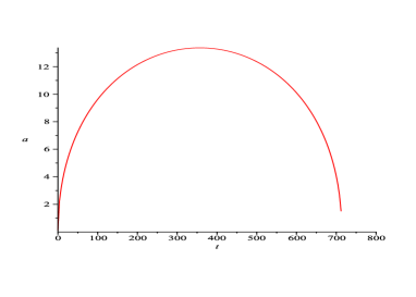
Figure 1: $a(t)$ as a function of $t$, for $\beta=0.1$, $E=1.336713605$, $a(t=0)=0.1$ and $\dot{a}(t=0)=6.650096751$.

In the present work, we study the quantum cosmology version of the noncommutative model described above. The noncommutativity, at the quantum level, we are about to propose will be between the canonically conjugated momenta to the scale factor and the radiative perfect fluid, following the choice made, at the classical level, by the authors of Ref. [31]. Since these variables are functions of the time coordinate $t$, this procedure is a generalization of the typical noncommutativity between usual spatial coordinates. The noncommutativity between those types of phase space variables have already been proposed in the literature. At the quantum level in Refs. [42, 43, 44, 45] and at the semi-classical and classical levels in Refs. [28, 29, 30, 31]. We quantize the model and obtain the appropriate Wheeler-DeWitt equation. In this model the scale factor takes values in a bounded domain. Therefore, its quantum mechanical version has a discrete energy spectrum. We compute the discrete energy spectrum and the corresponding eigenfunctions. The energies grow with a noncommutative parameter $\beta$. We compute the scale factor expected value ($\left<a\right>$) for several values of $\beta$. For all of them, $\left<a\right>$ oscillates between maxima and minima values and never vanishes. It gives an initial indication that those models are free from singularities, at the quantum level. We improve this result by showing that if we subtract a quantity proportional to the standard deviation of $a$ from $\left<a\right>$, this quantity is still positive. We observe that, $\left<a\right>$ grows with the decrease of $\beta$. We also observe that, the smaller the value of $\beta$, the greater is the interval where $\left<a\right>$ takes values. All these results confirm, at the quantum level, the results obtained in Ref. [31], for the scale factor, at the classical level. We also compute the Bohmian trajectories for $a$, which are in accordance with $\left<a\right>$, and the quantum potential $Q$. From $Q$, we may understand why that model is free from singularities, at the quantum level.

In the next section, we obtain the Wheeler-DeWitt equation for the NC model and solve it. The wavefunction is a linear combination of products of Airy functions and time exponentials. The number of terms contributing to the wavefunction is given by $N$. We compute the $\left<a\right>$ as a function of the NC parameter $\beta$ and $N$. We also compute, $\left<a\right>-\alpha\sigma_{a}$, where $\sigma_{a}$ stands for the standard deviation of $a$ and $\alpha$ is a real number. We show that for certain values of $\alpha$ this quantity is always positive, which improves the result that $\left<a\right>$ never goes to zero. In Section 3, we compute the Bohmian trajectories for $a$ and show that they are in accordance with $\left<a\right>$. We also compute the quantum potential $Q$. Studying $Q$, we show why that model is free from singularities, at the quantum level. Finally, in Section 4, we discuss the most important results of the present paper.

2 Quantum Cosmology in the Many Worlds Intepretation

The FRW cosmological models are characterized by the scale factor $a(t)$ and have the following line element,

$$ds^{2}=-N^{2}(t)dt^{2}+a^{2}(t)\left(\frac{dr^{2}}{1-kr^{2}}+r^{2}d\Omega^{2}\right)\,,$$ (4)

where $d\Omega^{2}$ is the line element of the two-dimensional sphere with unitary radius, $N(t)$ is the lapse function and $k$ gives the type of constant curvature of the spatial sections. Here, we are considering the case with zero curvature $k=0$ and we are using the natural unit system, where $\hbar=c=G=1$. The matter content of the model is represented by a perfect fluid with four-velocity $U^{\mu}=\delta^{\mu}_{0}$ in the comoving coordinate system used. The total energy-momentum tensor is given by,

$$T_{\mu,\,\nu}=(\rho+p)U_{\mu}U_{\nu}-pg_{\mu,\,\nu}\,,$$ (5)

where $\rho$ and $p$ are the energy density and pressure of the fluid, respectively. Here, we assume that $p=\rho/3$, which is the equation of state for radiation. This choice may be considered as a first approximation to treat the matter content of the early Universe and it was made as a matter of simplicity. It is clear that a more complete treatment should describe the radiation, present in the primordial Universe, in terms of the electromagnetic field.

From the metric (4) and the energy momentum tensor (5), one may write the total Hamiltonian of the present model ($N{\mathcal{H}}$), where $N$ is the lapse function and ${\mathcal{H}}$ is the superhamiltonian constraint. It is given by [48],

$$N{\mathcal{H}}=-\frac{p_{a}^{2}}{12}+p_{T},$$ (6)

where $p_{a}$ and $p_{T}$ are the momenta canonically conjugated to $a$ and $T$, the latter being the canonical variable associated to the fluid [47, 48]. Here, we are working in the conformal gauge, where $N=a$. The commutative version of the present model was first treated in Ref. [50].

We wish to quantize the model following the Dirac formalism for quantizing constrained systems [51]. First we introduce a wave-function which is a function of the canonical variables $a$ and $T$,

$$\Psi\,=\,\Psi(a,T)\,.$$ (7)

Then, we impose the appropriate commutators between the operators $a$ and $T$ and their conjugate momenta $p_{a}$ and $p_{T}$. Working in the Schrödinger picture, the operators $a$ and $T$ are simply multiplication operators, while their conjugate momenta are represented by the differential operators,

$$p_{a}\rightarrow-i\frac{\partial}{\partial a}\hskip 5.69046pt,\hskip 5.69046pt\hskip 5.69046ptp_{T}\rightarrow-i\frac{\partial}{\partial T}\hskip 5.69046pt.$$ (8)

Finally, we demand that the operator corresponding to $N\mathcal{H}$ annihilate the wave-function $\Psi$, which leads to the Wheeler-DeWitt equation,

$$\frac{1}{12}\frac{{\partial}^{2}}{\partial a^{2}}\Psi(a,\tau)=-i\,\frac{\partial}{\partial\tau}\Psi(a,\tau),$$ (9)

where the new variable $\tau=-T$ has been introduced. This is the Schrödinger equation of an one dimensional free particle restricted to the positive domain of the variable.

The operator $N\hat{\mathcal{H}}$ is self-adjoint [50] with respect to the internal product,

$$(\Psi,\Phi)=\int_{0}^{\infty}da\,\,\Psi(a,\tau)^{*}\,\Phi(a,\tau)\,,$$ (10)

if the wave functions are restricted to the set of those satisfying either $\Psi(0,\tau)=0$ or $\Psi^{\prime}(0,\tau)=0$, where the prime $\prime$ means the partial derivative with respect to $a$. Here, we consider wave functions satisfying the former type of boundary condition and we also demand that they vanish when $a$ goes to $\infty$. For the boundary conditions mentioned above, the author of Ref. [50] solved Eq. (9) and used that solution to compute $\left<a\right>$ for that model. He obtained, for the boundary condition $\Psi(0,\tau)=0$ (in the gauge $N=a$),

$$\left<a\right>=\frac{1}{6}\sqrt{\frac{2}{\pi\sigma}}\sqrt{\sigma^{2}\tau^{2}+(6-p\tau)^{2}},$$ (11)

where $\sigma$ is a positive number, $p$ is a real number and $\tau$ is the time variable. Therefore, $\left<a\right>$ starts from a nonzero value and when $\tau$ grows it also grows. Eventually, when $\tau\to\infty$ also $\left<a\right>\to\infty$. From Eq. (11), in that limit, $\left<a\right>\propto\tau$.

In order to introduce the noncommutativity in the present model, we shall modify the prescription used in Refs. [42, 43, 44, 45]. In those models the noncommutativity was described by a non-zero commutator between the operators associated to the canonical variables $a$ and $T$. Here, the non-zero commutator will be between the two operators associated to the canonical momenta $p_{a}$ and $p_{T}$,

$$\left[\breve{p_{a}},\breve{p_{T}}\right]=i\beta\,,$$ (12)

where $\breve{p_{a}}$ and $\breve{p_{T}}$ are the noncommutative versions of the operators and $\beta$ is the positive NC parameter. We follow, here, the choice compatible, at the quantum level, with the one made by the authors of Ref. [31], at the classical level. This noncommutativity between those operators can be taken to functions that depend on the noncommutative version of those operators with the aid of the Moyal product [52, 53, 7, 8]. Consider two functions of $\breve{a}$ and $\breve{T}$, let’s say, $f$ and $g$. Then, the Moyal product between those two function is given by: $f(\breve{a},\breve{T})\star g(\breve{a},\breve{T})=f(\breve{a},\breve{T})\exp{\left[(i\theta/2)(\overleftarrow{\partial_{\breve{a}}}\overrightarrow{\partial_{\breve{T}}}-\overleftarrow{\partial_{\breve{T}}}\overrightarrow{\partial_{\breve{a}}})\right]}g(\breve{a},\breve{T})$.

Using the Moyal product, we may adopt the following Wheeler-DeWitt equation for the noncommutative version of the present model,

$$\left[\frac{1}{12}\breve{p}_{a}\star\breve{p}_{a}-\breve{p}_{T}\right]\star\Psi(\breve{a},\breve{T})=0.$$ (13)

It is possible to rewrite the Wheeler-DeWitt equation (13) in terms of a commutative version of the operators $\breve{p_{a}}$ and $\breve{p_{T}}$ and the ordinary product of functions. In order to do that, we must initially introduce the following transformation between the noncommutative and the commutative operators,

$$\breve{p_{a}} = p_{a}+\beta T,$$ (14)

$$\breve{p_{T}} = p_{T},$$

and the transformations of the other noncommutative variables are trivial: $\breve{a}=a$ and $\breve{T}=T$. We follow, here, the choice compatible, at the quantum level, with the one made by the authors of Ref. [31], at the classical level. Then, we may write the commutative version of the Wheeler-DeWitt equation (13), to first order in the commutative parameter $\beta$, in the Schrödinger picture as,

$$\frac{1}{12}\frac{\partial^{2}\Psi(a,\tau)}{\partial a^{2}}-\frac{i}{6}\beta\tau\frac{\partial\Psi(a,\tau)}{\partial a}=-i\frac{\partial\Psi(a,\tau)}{\partial\tau},$$ (15)

where we have made the following transformation $\tau\to-T$, in the same way the author of Ref. [50], so that, we may compare the $\left<a\right>$ computed using our solution with Eq. (11). For a vanishing $\beta$ this equation reduces to the commutative Schrödinger equation (9), described above.

In order to solve this equation, satisfying the boundary conditions: $\Psi(0,\tau)=0$ and $\lim_{a\to\infty}\Psi(a,\tau)\to 0$, we start imposing that the wave function $\Psi(a,\tau)$ has the following form,

$$\Psi(a,\tau)=e^{i\beta a\tau}e^{-iE\tau}A(a).$$ (16)

Introducing this ansatz in Eq. (15), we obtain, to first order in $\beta$, the eigenvalue equation,

$$\frac{d^{2}A(a)}{da^{2}}-(12\beta a-12E)A(a)=0,$$ (17)

where $E$ is the eigenvalue and it is associated with the fluid energy.

The solutions to this equation are the Airy functions,

$$A(a)=c_{1}Ai\left(\frac{12\theta a-12E}{(12\beta)^{2/3}}\right)+c_{2}Bi\left(\frac{12\theta a-12E}{(12\beta)^{2/3}}\right).$$

The Airy functions $Bi$ grow up exponentially when $a\rightarrow\infty$. In order to eliminate this undesirable behavior, we put $c_{2}=0$. Then, the energy eigenfunctions for our model are,

$$A(a)=c_{1}Ai\left(\frac{12\beta a-12E}{(12\beta)^{2/3}}\right).$$ (18)

If we introduce the boundary condition that $A(a=0)=0$, we find from Eq. (18) the energy eigenvalues with the following expression,

$$E_{n}=\frac{1}{12}(12\beta)^{2/3}\alpha_{n}$$ (19)

where $\alpha_{n}$ is positive and is the zero of order $n$ of the Airy function $Ai$. It is clear from this equation that the energy eigenvalues grow with $\beta$.

The most general expression of $\Psi(a,\tau)$ Eq. (16), which is a solution to Eq. (15), is a linear combination of the eigenfunctions $A_{n}(a)$, Eq. (18), taking in account the energy eigenvalues Eq. (19), combined with the exponential factor present in Eq. (16), for a given $\beta$ value.

$$\Psi(a,\tau)=e^{i\beta a\tau/2}\sum_{n=0}^{N}C_{n}Ai\left(\frac{12\beta a-12E_{n}}{(12\beta)^{2/3}}\right)\exp{(-iE_{n}\tau)}.$$ (20)

In order to build a wave packet from Eq. (20) one has, initially, to fix the values of $\beta$ and the number $N$ of energy eigenfunctions contributing to the sum. After that, one has to compute the $N$ energy eigenvalues $E_{n}$ Eq. (19), with the aid of the first $N$ zeros ($\alpha_{n}$) of the Airy function $Ai$. Also, one has to fix the values of the $N$ coefficients $C_{n}$. Finally, one has to introduce the explicit values of all those quantities in Eq. (20) and perform the indicated sum. The time evolution of the wave packets built from Eq. (20) shows that they are null not only at the origin but they are asymptotically null at infinity as well. In the region near $a=0$ these packets present strong oscillations, which decrease as $a$ increases.

Now, we shall use the wavefunction (20) in order to compute some important quantities. Initially, we shall compute, the scale factor expected value, $\left<a\right>$, for different values of $\beta$ and $N$. First of all, let us choose $C_{n}=1$, for all $n$, in Eq. (20). In fact, we shall do this choice for the $C_{n}$’s coefficients in all calculations in this paper. Next, we compute the eigenvalues, $E_{n}$, with the aid of Eq. (19). In order to do that we must choose the values of $\beta$, $N$ and $\alpha_{n}$. In the present situation, we shall choose several different values of $\beta$ and $N$. Finally, we must compute the scale factor expected value, using the following expression,

$$\left<a\right>=\frac{\int_{0}^{\infty}a\,|\Psi(a,\tau)|^{2}da}{\int_{0}^{\infty}|\Psi(a,\tau)|^{2}da}.$$ (21)

After computing $\left<a\right>$ for several different values of $\beta$, $N$ and various $\tau$ intervals, we noticed that this quantity oscillates between maxima and minima values and never vanishes. It gives an initial indication that those models are free from singularities, at the quantum level. Now, if we fix $N$ and vary $\beta$ we observe the following properties of $\left<a\right>$: ($i$) the maximum value of $\left<a\right>$ decreases with the increase of $\beta$; ($ii$) the amplitude of oscillation for $\left<a\right>$ decreases with the increase of $\beta$; ($iii$) the number of $\left<a\right>$ oscillations, for a fixed $\tau$ interval, increases with the increase of $\beta$. Those behaviors may be understood by the fact that the potential barrier, that confines the scale factor, grows linearly with $\beta$. Therefore, as $\beta$ increases the $\left<a\right>$ is forced to oscillate in an ever decreasing region. Under those conditions, for fixed $N$, the maximum value and the amplitude of $\left<a\right>$ decrease. Also, since the domain where $\left<a\right>$ oscillates is decreasing, the number of $\left<a\right>$ oscillations, for a fixed $\tau$ interval, increases. All those properties can be seen in Figures 2 and 3. Each figure shows the behavior of $\left<a\right>$ for a different value of $\beta$ while the $\tau$ interval and $N$ remain fixed. Now, if we fix $\beta$ and vary $N$ we observe the following properties of $\left<a\right>$: ($i$) the maximum value of $\left<a\right>$ grows with the increase of $N$; ($ii$) the amplitude of oscillation for $\left<a\right>$ increases with the increase of $N$; ($iii$) the number of $\left<a\right>$ oscillations, for a fixed $\tau$ interval, decreases with the increase of $N$. In order to understand those behaviors we notice that the mean energy associated with the wavepacket increases with the increase of $N$. Therefore, for fixed $\beta$, when we increase $N$ the domain where $\left<a\right>$ oscillates increases. In this way, the maximum value and the amplitude of $\left<a\right>$ increase. On the other hand, the number of $\left<a\right>$ oscillations, for a fixed $\tau$ interval, decreases. All those properties can be seen in Figures 4 and 5.

As we have mentioned above, for all values of $\beta$ and $N$ considered, $\left<a\right>$ never vanishes. It gives an initial indication that those models are free from singularities, at the quantum level. We may improve this result by computing $\left<a\right>-\alpha\sigma_{a}$, where $\sigma_{a}$ stands for the standard deviation of $a$ and $\alpha$ is a positive real number. If this quantity is always positive like $\left<a\right>$, it will be a stronger indication that the model is free from singularities, at the quantum level. Let us compute $\left<a\right>-\alpha\sigma_{a}$, for the present model. By definition the standard deviation of $a$ is given by,

$$\sigma_{a}=\sqrt{\left<a^{2}\right>-\left<a\right>^{2}},$$ (22)

where,

$$\left<a^{2}\right>=\frac{\int_{0}^{\infty}a^{2}\,|\Psi(a,\tau)|^{2}da}{\int_{0}^{\infty}|\Psi(a,\tau)|^{2}da},$$ (23)

and $\left<a\right>^{2}$ is given by the square of Eq. (21). Using the wavefunction (21) and repeating some procedures we did in order to compute $\left<a\right>$, we computed $\left<a\right>-\alpha\sigma_{a}$ for several values of $\alpha$, $\beta$ and $N$. The result is that for the huge majority of cases this quantity is always positive. More precisely, if $\alpha\leq 3/4$, in the interval $10^{-7}\leq\beta\leq 0.5$, $\left<a\right>-\alpha\sigma_{a}$ is always positive for any value of $N$. As for the mathematical significance of $\alpha=3/4$, we may mention that if our distribution were a normal one and if one takes the interval $\left<a\right>\pm\alpha\sigma_{a}$, around the mean value, it would cover over half the area under the distribution. More precisely, $54,67\%$ [54]. Two examples of $\left<a\right>-3\sigma_{a}/4$, as a function of time, are shown in Figures 6 and 7.

Therefore, we notice that the introduction of the noncommutativity represented by Eq. (12) modified in an important way the commutative version of the model. In the commutative version of the model the scale factor expected value takes values in an unbounded domain. It expands as the function of $\tau$ given by Eq. (11). On the other hand, in the noncommutative version of the model the scale factor mean value takes values in a bounded domain and is periodic in $\tau$. The commutative version of the model may be obtained from the noncommutative one by taking the limit when $\beta\to 0$. The above results show clearly that limit from one version to the other. If we start decreasing the value of $\beta$ the scale factor expected value will oscillate in an ever increasing domain until we set $\beta\to 0$. At that limit Eq. (15) reduces to Eq. (9) and the scale factor expected value will grow without limits, as the function of $\tau$ given by Eq. (11).

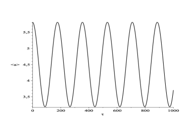
Figure 2: $\left<a\right>$ for $\beta=0.01$, $N=2$ and the time interval $0\leq\tau\leq 1000$.

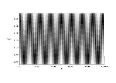
Figure 3: $\left<a\right>$ for $\beta=0.5$, $N=2$ and the time interval $0\leq\tau\leq 1000$.

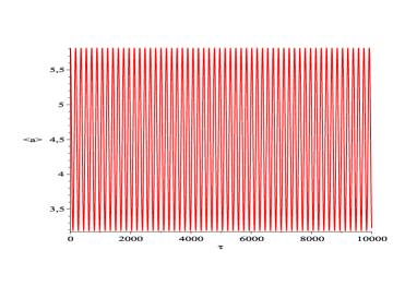
Figure 4: $\left<a\right>$ for $N=2$, $\beta=0.01$ and the time interval $0\leq\tau\leq 10000$.

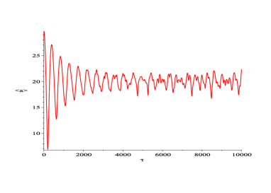
Figure 5: $\left<a\right>$ for $N=22$, $\beta=0.01$ and the time interval $0\leq\tau\leq 10000$.

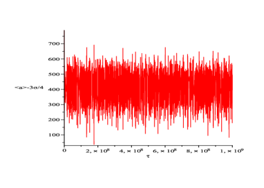
Figure 6: $\left<a\right>-3\sigma_{a}/4$ for $N=15$, $\beta=0.0000001$ and the time interval $0\leq\tau\leq 10^{9}$.

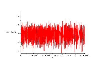
Figure 7: $\left<a\right>-3\sigma_{a}/4$ for $N=20$, $\beta=0.5$ and the time interval $0\leq\tau\leq 10^{9}$.

3 Quantum Cosmology in the DeBroglie-Bohm Intepretation

In this section, we want to apply the DeBroglie-Bohm interpretation of quantum mechanics, to the present NC quantum cosmology model. Our main motivation is to compare the results we shall obtain with that interpretation with the ones we obatined in the previous section, where we used the Many Worlds interpretation of quantum mechanics. In order to use the DeBroglie-Bohm interpretation we must re-write $\Psi(a,\tau)$ Eq. (20), in the polar form,

$$\Psi(a,\tau)=R(a,\tau)e^{iS(a,\tau)}$$ (24)

where,

$$R(a,\tau)=\sqrt{\sum_{n,m=0}^{N}C_{n}C_{m}Ai\left(G\left(\beta,E_{n},a\right)\right)Ai\left(G\left(\beta,E_{m},a\right)\right)\cos\left((E_{n}-E_{m})\tau\right)}$$ (25)

$$S(a,\tau)=\arctan\left[\frac{-\sum_{n=0}^{N}C_{n}Ai\left(G\left(\beta,E_{n},a\right)\right)\sin(E_{n}\tau)}{\sum_{m=0}^{N}C_{m}Ai\left(G\left(\beta,E_{m},a\right)\right)\cos(E_{m}\tau)}\right].$$ (26)

where $G\left(\beta,E_{n},a\right)=\left(12\beta a-12E_{n}\right)/(12\beta)^{2/3}$.

Following the DeBroglie-Bohm interpretation we introduce $\Psi(a,\tau)$ Eq. (24) in Eq. (15), this leads to the next two equations for $R(a,\tau)$ and $S(a,\tau)$ [55],

$$12\frac{\partial S(a,\tau)}{\partial\tau}-2\beta\tau\frac{\partial S(a,\tau)}{\partial a}+\left(\frac{\partial S(a,\tau)}{\partial a}\right)^{2}+Q(a,\tau) = 0,$$ (27)

$$\frac{\partial R(a,\tau)}{\partial\tau}+\frac{1}{6}\frac{\partial S(a,\tau)}{\partial a}\frac{\partial R(a,\tau)}{\partial a}+\frac{1}{12}R(a,\tau)\frac{\partial^{2}S(a,\tau)}{\partial a^{2}}-\frac{1}{6}\beta\tau\frac{\partial R(a,\tau)}{\partial a} = 0,$$ (28)

where the Bohmian quantum potential $Q(a,\tau)$ is defined by [55],

$$Q(a,\tau)=-\frac{1}{R(a,\tau)}\frac{\partial^{2}R(a,\tau)}{\partial a^{2}}.$$ (29)

In the present situation, using the value of $R(a,\tau)$ Eq. (25), $Q(a,\tau)$ Eq. (29) takes the form,

$$Q(a,\tau)=\frac{1}{4}\frac{1}{M_{1}^{2}}\left(\frac{\partial M_{1}}{\partial a}\right)^{2}-\frac{1}{2}\frac{1}{M_{1}}\frac{\partial^{2}M_{1}}{\partial a^{2}},$$ (30)

where

$$M_{1}=\sum_{n,m=0}^{N}C_{n}C_{m}\ Ai\left(G(\beta,E_{n},a)\rule{0.0pt}{11.38109pt}\right)Ai\left(G(\beta,E_{m},a)\rule{0.0pt}{11.38109pt}\right)\cos\left((E_{n}-E_{m})\tau\rule{0.0pt}{11.38109pt}\right).$$ (31)

The Bohmian trajectory for $a$ is given by [55],

$$\frac{da(\tau)}{d\tau}=\frac{1}{m}\frac{\partial S}{\partial a},$$ (32)

where, from Eq. (6) $m$ for the present situation is given by $6$. Using the value of $S(a,\tau)$ Eq. (26) in Eq. (32), it reduces to,

$$\frac{da(\tau)}{d\tau}=\frac{1}{6}\frac{F_{3}(\tau)}{F_{4}(\tau)}$$ (33)

where,

$$F_{3}(\tau) = \sum_{n,m=0}^{N}C_{n}C_{m}{Ai}^{\prime}\left(G\left(\beta,E_{{n}},a\left(\tau\right)\right)\rule{0.0pt}{11.38109pt}\right){Ai}\left(G\left(\beta,E_{{m}},a\left(\tau\right)\right)\rule{0.0pt}{11.38109pt}\right)\times$$ (34)

$$\times\sin\left(\left(E_{{n}}-E_{{m}}\right)\tau\rule{0.0pt}{11.38109pt}\right),$$

$$F_{4}(\tau) = \left[\sum_{n=0}^{N}C_{n}{Ai}\left(G\left(\beta,E_{{n}},a\left(\tau\right)\right)\rule{0.0pt}{11.38109pt}\right)\cos\left(E_{n}\tau\right)\right]^{2}+$$ (35)

$$\left[\sum_{m=0}^{N}C_{m}Ai\left(G\left(\beta,E_{{m}},a\left(\tau\right)\right)\rule{0.0pt}{11.38109pt}\right)\sin\left(E_{{m}}\tau\right)\right]^{2}.$$

The solution to Eq. (33), which is the Bohmian trajectory of $a(\tau)$, which is the variable describing the universe, represents the quantum behavior for the cosmic evolution in the Planck era.

We solved Eq. (33) for many different values of $\beta$ and $N$, the number of energy eigenfunctions contributing to the wavefunction Eq. (24). We found the same qualitative behavior for the Bohmian trajectories of $a(\tau)$, in all those cases. It oscillates between maxima and minima values and never goes through the zero value. It means that, quantum mechanically, in those models there are no singularities which confirms the result obtained in the previous section using the Many Worlds interpretation. In order to exemplify this behavior we show the Bohmian trajectories of $a(\tau)$ for two models with $N=2$ and $\beta=0.01$, Figure 8, and $\beta=0.5$, Figure 9. We computed the time evolution of $a(\tau)$ up to $t=1000$ and used the initial conditions for $a(\tau)$ at $\tau=0$, obtained from the calculation of the expected value of $a(\tau)$, for the corresponding models. The results shown in Figures 8 and 9 are qualitatively very similar to Figures 2 and 3, that represent the scale factor expected values for the corresponding models. For different values of $N$, the behavior of $a(\tau)$ is also qualitatively very similar to the behavior of $\left<a\right>$. As an example, we show $a(\tau)$, Figure 10, for the model where $N=22$, $\beta=0.01$, $0\leq\tau\leq 10000$ and the initial condition for $a(\tau)$ at $\tau=0$ was obtained from the calculation of $\left<a\right>$. This Figure must be compared with Figure 5, for $\left<a\right>$ of the corresponding model.

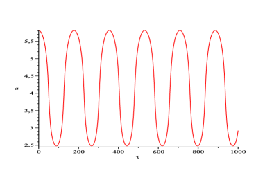
Figure 8: $a(\tau)$ for $N=2$, $\beta=0.01$, the initial condition $a(\tau=0)=5.814364999$ and the time interval $0\leq\tau\leq 1000$.

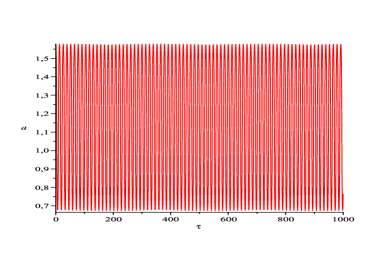
Figure 9: $a(\tau)$ for $N=2$, $\beta=0.5$, the initial condition $a(\tau=0)=1.578261478$ and the time interval $0\leq\tau\leq 1000$.

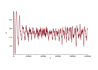
Figure 10: $a(\tau)$ for $N=22$, $\beta=0.01$, the initial condition $a(\tau=0)=29.71117629$ and the time interval $0\leq\tau\leq 10000$.

The absence of singularities in the present models are very easy to understand when one observes the Bohmian quantum potential Eq. (30), for those models. We computed $Q(a,\tau)$ Eq. (30), for several values of $\beta$ and $N$. The calculations were made over the Bohmian trajectories of $a$. We obtained $Q$ as a function of $\tau$ as well as a function of $a$. We found the same qualitative behavior of $Q$, in all those cases. Initially, considering $Q$ as a function of $\tau$, at $\tau=0$, there is a potential barrier ($B_{0}$) that prevents the value of $a$ ever to go through zero. Then, the barrier becomes a well for a brief moment and again a new barrier appears ($B_{1}$). After a while, $B_{1}$ turns into a well for a brief moment and then another barrier identical to $B_{0}$ appears. After that, $Q$, periodically, repeats itself. $B_{0}$ is different from $B_{1}$. $B_{1}$ exists for a longer period and is shorter than $B_{0}$. One may interpret the potential shape in the following way. Initially, at $\tau=0$, $a$ starts to grow from its minimum value different from zero, first rapidly, and then its velocity starts to decrease until it goes to zero, at the maximum value of $a$. Then, $a$ starts to decrease, first slowly, and then its velocity starts to increase until $a$ reaches its minimum value different from zero. There, its velocity changes sign and $a$ starts to grow once more, as described above. This dynamics is represented in $Q$, initially, by $B_{0}$, then the first well, then $B_{1}$ and finally the well just after $B_{1}$. Then, the movement of $a$ repeats itself periodically. These models have no singularities because $B_{0}$ and its periodic repetitions prevent $a$ ever to go through zero. In order to exemplify this behavior we show, in Figure 11, the Bohmian quantum potential Eq. (30), for the model with $\beta=0.1$ and $N=2$. For a better visualization of $Q$’s behavior, we choose a small time interval in Figure 11. We computed, also, $Q$ as a function of $a$. In this case, we may see clearly $B_{0}$ and $B_{1}$. In Figure 12, we show $Q$ as a function of $a$, for the model with $\beta=0.1$ and $N=2$. For a clearer understand of $Q$’s behavior we plotted, in Figure 13, the Bohmian trajectory of $a$ used in order to compute $Q$ given in Figures 11 and 12. $a$, Figure 13, is plotted during the same time interval of $Q$, Figure 11, and its initial condition $a(\tau)$ at $\tau=0$, was obtained from the calculation of the expected value of $a$, for the same model.

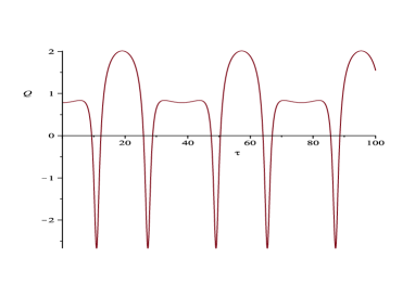
Figure 11: $Q(\tau)$ for $N=2$, $\beta=0.1$ and the time interval $0\leq\tau\leq 100$.

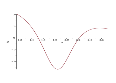
Figure 12: $Q(a)$ for $N=2$, $\beta=0.1$ in the $a$ interval $1.150667559\leq a\leq 2.698789166$.

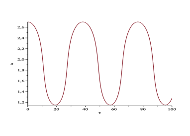
Figure 13: $a(\tau)$ for $N=2$, $\beta=0.1$, the initial condition $a(\tau=0)=2.698789166$ and the time interval $0\leq\tau\leq 100$.

4 Conclusions

The above results indicate that, also at the quantum level, the scale factor may have been, initially, bounded, due to the presence of noncommutativity. The difference between the scale factor behavior at the classical and the quantum levels is the fact that, in the quantum NC version of the model both the scale factor expected value and its Bohmian trajectory oscillate between maxima and minima values and never go to zero. Therefore, this NC cosmological model is free from singularities, at the quantum level. In the many words interpretation, it is possible to improve this result by showing that the quantity $\left<a\right>-\alpha\sigma_{a}$ is always positive for many values of $\alpha$. Where $\sigma_{a}$ stands for the standard deviation of $a$ and $\alpha$ is a positive real number. From the quantum potential $Q$, for that NC model, it is easy to see why the Bohmian trajectory for $a$ never goes to zero. On the other hand, in the classical NC version of the present model, the scale factor starts expanding from a minimum value, then reachs a maximum value and finally contracts to zero, giving rise to a singularity. It is important to investigate if other types of noncommutativity applied to models with the conditions present in our early Universe, also give rise to scale factors which take values in a bounded domain. That would indicate an important prediction of NC cosmological models about the early universe. In this sense, we may mention that in a previous work [45] the authors quantized a noncommutative FRW model with $k=1$ and radiation. For a noncommutativity described by a non-zero commutator between the scale factor ($a$) and the variable associated to the radiative fluid ($T$), they showed that it is not possible to solve the Wheeler-DeWitt equation for that model and find a wavefunction, with the boundary condition $\Psi(0,T)=0$.

Acknowledgements. M. Silva de Oliveira thanks CAPES for her scholarship. G. A. Monerat thank UERJ for the Prociencia grant.

References

- [1] H. S. Snyder, Phys. Rev. 71, 38 (1947).
- [2] H. S. Snyder, Phys. Rev. 72, 68 (1947).
- [3] T. Banks, W. Fischler, S. H. Shenker, and L. Susskind, Phys. Rev. D 55, 5112 (1997).
- [4] A. Connes, M. R. Douglas, and A. Schwarz, J. High Energy Phys. 02, 003 (1998).
- [5] C. S. Chu and P. M. Ho, Nucl. Phys. B550, 151 (1999).
- [6] V. Schomerus, J. High Energy Phys. 06, 030 (1999).
- [7] N. Seiberg and E. Witten, J. High Energy Phys. 09, 032 (1999).
- [8] M. R. Douglas, N. A. Nekrasov, Rev. Mod. Phys. 73, 977 (2001).
- [9] R. J. Szabo, Phys. Rep. 378, 207 (2003).
- [10] V. P. Nair, A. P. Polychronakos, Phys. Lett. B 505, 267 (2001).
- [11] J. Gamboa, M. Loewe, J. C. Rojas, Phys. Rev. D 64, 067901 (2001).
- [12] S. Bellucci, A. Nersessian, C. Sochichiu, Phys. Lett. B 522, 345 (2001).
- [13] M. Chaichian, M. M. Sheikh-Jabbari, A. Tureanu, Phys. Rev. Lett. 86, 2716 (2001).
- [14] O. F. Dayi and A. Jellal, J. Math. Phys. 43, 4592 (2002).
- [15] O. F. Dayi and A. Jellal, J. Math. Phys. 45, 827(E) (2004).
- [16] A. Kokado, T. Okamura, T. Saito, Prog. Theor. Phys. 110, 975 (2003).
- [17] A. H. Chamseddine, Phys. Lett. B 504, 33 (2001).
- [18] P. Aschieri, C. Blohmann, M. Dimitrijević, F. Meyer, P. Schupp and J. Wess, Class. Quantum Grav. 22, 3511 (2005).
- [19] P. Aschieri, M. Dimitrijević, F. Meyer and J. Wess, Class. Quantum Grav. 23, 1883 (2006).
- [20] R. Brandenberger and P. M. Ho, Phys. Rev. D 66, 023517 (2002).
- [21] Q. G. Huang and M. Li, JHEP 0306, 014 (2003).
- [22] H. Kim, G. S. Lee, H. W. Lee and Y. S. Myung, Phys. Rev. D 70, 043521 (2004).
- [23] D. Liu and X. Li, Phys. Rev. D 70, 123504 (2004).
- [24] Q. G. Huang and M. Li, Nucl. Phys. B 713, 219-234 (2005).
- [25] H. Kim, G. S. Lee and Y. S. Myung, Mod. Phys. Lett. A 20, 271-283 (2005).
- [26] W. Nelson and M. Sakellariadou, Phys. Lett. B 680, 263-266 (2009).
- [27] K. Nozari and S. Akhshabi, Phys. Lett. B 700, 91-96 (2011).
- [28] B. Vakili, P. Pedram and S. Jalalzadeh, Phys. Lett. B 687, 119 (2010).
- [29] O. Obregon and I. Quiros, Phys. Rev. D 84, 044005 (2011).
- [30] C. Neves, G. A. Monerat, E. V. Corrêa Silva, L. G. Ferreira Filho, e-print arXiv:gr-qc/1109.3514 (2011).
- [31] E. M. C. Abreu, M. V. Marcial, A. C. R. Mendes, W. Oliveira and G. Oliveira-Neto, JHEP 05, 144 (2012).
- [32] P. Nicolini, J. Phys. A 38, L631 (2005).
- [33] P. Nicolini, A. Smailagic and E. Spallucci, Phys. Lett. B 632, 547 (2006).
- [34] S. Ansoldi, P. Nicolini, A. Smailagic and E. Spallucci, Phys. Lett. B 645, 261 (2007).
- [35] T. G. Rizzo, JHEP 09, 021 (2006).
- [36] M. Chaichian, A. Tureanu and G. Zet, Phys. Lett. B 660, 573 (2008).
- [37] E. Spallucci, A. Smailagic and P. Nicolini, Phys. Lett B 670, 449 (2009).
- [38] R. Banerjee, B. R. Majhi and S. K. Modak, Class. Quantum Grav. 26, 085010 (2009).
- [39] P. Nicolini, Int. J. Mod. Phys. A 24, 1229 (2009).
- [40] R. Banerjee, S. Gangopadhyay and S. K. Modak, Phys. Lett. B 686, 181 (2010).
- [41] E. Brown and R. Mann, Phys. Lett. B 694, 440 (2011).
- [42] H. Garcia-Compean, O. Obregon and C. Ramirez, Phys. Rev. Lett. 88, 161301 (2002).
- [43] G. D. Barbosa and N. Pinto-Neto, Phys. Rev. D 70, 103512 (2004).
- [44] G. D. Barbosa, Phys. Rev. D 71, 063511 (2005).
- [45] G. Oliveira-Neto, G. A. Monerat, E. V. Corrêa Silva, C. Neves, L. G. Ferreira Filho, e-print arXiv:gr-qc/1206.5029 (2012).
- [46] R. Banerjee, B. Chakraborty, S. Ghosh, P. Mukherjee, S. Samanta, Found. Phys. 39, 1297 (2009).
- [47] Schutz, B. F., Phys. Rev. D 2, 2762 (1970); Schutz, B. F., Phys. Rev. D 4, 3559 (1971).
- [48] F. G. Alvarenga, J. C. Fabris, N. A. Lemos, G. A. Monerat, Gen. Rel. Grav. 34, 651 (2002).
- [49] R. D’Inverno, Introducing Einstein’s Relativity, (Oxford University Press, Oxford, 1995).
- [50] N. A. Lemos, J. Math. Phys. 37, 1449 (1996).
- [51] P. A. M. Dirac, Can. J. Math. 2, 129 (1950); Proc. Roy. Soc. London A 249, 326 and 333 (1958); Phys. Rev. 114, 924 (1959).
- [52] J. E. Moyal, Proc. Cambridge Phil. Soc. 45, 99 (1949).
- [53] F. Bayen, M. Flato, C. Fronsdal and A. Lichnerowicz, Ann. Phys. 111, 61 (1978).
- [54] P. L. Meyer, Introductory Probability and Statistical Applications, (Addison-Wesley, Reading, 1970).
- [55] P. R. Holland, The quantum theory of motion: an account of the de Broglie-Bohm interpretation of quantum mechanics, (Cambridge University Press, Cambridge, 1993).