Characterizing weak chaos in nonintegrable Hamiltonian systems:
the fundamental role of stickiness and initial conditions

Abstract

Weak chaos in high-dimensional conservative systems can be characterized through sticky effect induced by invariant structures on chaotic trajectories. Suitable quantities for this characterization are the higher cummulants of the finite time Lyapunov exponents (FTLEs) distribution. They gather the whole phase space relevant dynamics in one quantity and give informations about ordered and random states. This is analyzed here for discrete Hamiltonian systems with local and global couplings. It is also shown that FTLEs plotted versus initial condition (IC) and the nonlinear parameter is essential to understand the fundamental role of ICs in the dynamics of weakly chaotic Hamiltonian systems.

1 Introduction

The phase space of nonlinear conservative Hamiltonian systems can present regions of regular, mixed and chaotic motion, depending on the nonlinear parameter. The regular region is characterized by the complete absence of chaotic trajectories while the chaotic region by the absence of regular trajectories, with exceptions of measure zero stable orbits. The mixed regions on the other hand, contains simultaneously the regular and chaotic motion (or quasi-regular) and everything becomes complicated [1, 2]: the positions of regular structures, their size distribution, exit times, the shapes of the structures boundaries and the penetration inside them which is possible in higher dimensions. Weak chaos occurs in the mixed region where an approximately even competition between the regular and chaotic dynamics occurs [1]. In $2-$dimensional conservative problems ($4-$dimensional phase space) the dynamics can be described by using the technique of Poincaré Surfaces of Section (PSS). However, for high-dimensional systems this technique is only partially useful due to the restriction of plots to $2-$ and $3-$dimensions, which makes it almost impossible to construct adequate PSSs which allow to describe the whole dynamics. Beside that, $3-$dimensional plots of high-dimensional systems are fairly unsatisfactory projections from the whole system. A recent work proposes visualization of classical structures using phase space slices [3].

Another possibility is to use Lyapunov quantifiers which decide if a trajectory is chaotic or not. In the mixed region stickiness [4, 5] affects the convergence of finite time Lyapunov exponents (FTLEs), but they contain essential informations about the properties of the regular structures which live in the high-dimensional phase space. The properties of regular structures have been addressed on the same constant energy [6], by studying their dimensionality [7, 8], and the almost invariant sets in continuous problems [9, 10], to mention a few. The purpose of the present work is not to describe the invariant structures itself, but to quantify their effect on the dynamics. As explained below, it turns out that FTLEs are very suitable to do the job in the mixed regions. Any dynamical evolution of the system depends on the starting point in phase space and on the shape and number of regular structures of its surroundings. Since FTLEs are usually strongly dependent on the initial conditions (ICs) and on the sticky motion, they can be used to quantify the amount of regular motion in high-dimensional phase spaces. It would be nice to check the stickiness influence on the smaller alignment index [11, 12] which rapidly distinguish between ordered and chaotic trajectories in Hamiltonian flows.

A very appropriate way to quantify the sticky motion is by analyzing higher order cummulants of the FTLEs distribution. This was proposed [13] for the standard map and applied [14] to higher dimensions in conservative non-Hamiltonian systems. It was found [14] by this technique that for $2,4,10$ and $20$ phase space dimensions, conservative coupled standard maps with unidirectional local coupling can be characterized of being chaotic, quasi-regular or regular. In addition, for some values of the nonlinear parameter in the quasi-regular region, stickiness is shown to affect all unstable directions simultaneously and by the same amount, which is quantified by the cummulants mentioned above. This remarkable property was named common behavior [14] and its main property is that regular structures in phase space “attract” the chaotic trajectories by the amount in all unstable directions. Once the chaotic trajectory is attracted, it remains sticked to the regular structure and then presents the clustering behavior observed [15] in conservative maps. But the essential new property from the common behavior is that the rate of attraction of the chaotic trajectory into the regular structure is equal in different unstable directions.

The question remains if the common motion is a general property found also in Hamiltonian and symplectic systems, or maybe it depends on the particular choice of the coupling? In order to answer this question and to understand better mixed phase spaces, in this work we extend our method to Hamiltonian systems with global and local couplings and compare the results. The existence of an additional constant of motion, besides the total energy, allows for a clear interpretation of results.

The paper is divided in the following way. In Section 2 the local and global coupled maps models used in this work are presented and in Section 3 we summary the main properties of the FTLEs distribution in order to detect stickiness. In Section 4 we present and discuss the results which are summarized in the conclusions in Section 5.

2 Lattices of Coupled Hamiltonian Maps

The model we investigate is conservative with an additional constant of motion. It describes $N$ particles coupled on a unit circle, where the state of each particle is defined by its position $x^{(i)}$ and its conjugate momentum $p^{(i)}$. The lattice of $N$ coupled maps is written as

$$\left\{\begin{array}[]{ll}p_{t+1}^{(i)}=p_{t}^{(i)}+f(x_{t})\qquad\mbox{mod}\,1,\\ \\ x_{t+1}^{(i)}=x_{t}^{(i)}+p_{t+1}^{(i)}\,\,\qquad\mbox{mod}\,1,\end{array}\right.$$ (4)

where $f(x_{t})$ can be local or global coupling as discussed next. The local coupling (LC) is defined accordingly to

$$f(x_{t})=\frac{K}{2\pi} \left\{\sin[2\pi(x_{t}^{(i+1)}-x_{t}^{(i)})]\right.$$ (5)

$$- \left.\sin[2\pi(x_{t}^{(i)}-x_{t}^{(i-1)})]\right\},$$

where $i=1,\ldots,N$. We considered periodic boundary conditions $p^{(N+1)}=p^{(1)},x^{(N+1)}=x^{(1)}$. Some properties of this model were already investigated numerically in [16, 17, 18]. For the global coupling (GC) we have

$$f(x_{t})=\frac{K}{2\pi\sqrt{N-1}}\sum_{j=1,j\not=i}^{N}\sin[2\pi(x_{t}^{(j)})-2\pi(x_{t}^{(i)})],$$ (7)

where $i=1,\ldots,N$ [17] . $K$ is simultaneously the nonlinear parameter and the coupling strength between distinct sites. For $K>0$ the interaction term $f(x_{t})$ between two particles $i$ and $j$ is attractive [19]. Both models have the total momentum $P_{T}=\sum_{j=1}^{N}p^{j}_{t}$ as a conservative quantity and they were extensively studied in [19, 20], which characterized the system by the existence of an ordering process called cluster, which will be discussed later.

3 Stickiness and the FTLEs distributions

In this Section we summarize the method used to detect stickiness from the FTLEs distribution. Sticky motion reduces the local FTLE along a chaotic trajectory. This can be seen in Fig. 1, where the FTLEs are plotted as a function of time. In this case simulations were realized for the GC with $N=4$, $K=1.0$ [Fig. 1(a)] and $K=0.21$ [Fig. 1(b)]. After the last iteration the corresponding FTLEs distribution over initial conditions is plotted (in red). As time increases the local FTLE increases for a chaotic trajectory, but since it may touch or penetrate regular structures in the phase space, sticky motion occurs and the local FTLE decreases (see green decreasing lines). When this trajectory leaves the sticky region, the local FTLE starts to increase again. Thus, those chaotic trajectories affected by the sticky motion will have smaller values of their FTLEs at the last iteration. This induces a small tail to the right in the distribution of the FTLEs [see Fig. 1(a)], and it becomes asymmetric. Therefore, while for intermediate values of $K$ such asymmetric fat tails are expected, for larger $K$ values, where a totally chaotic motion occurs, a Gaussian distribution for the FTLEs is expected.

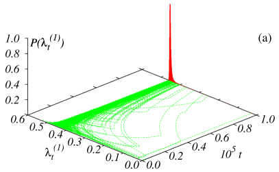
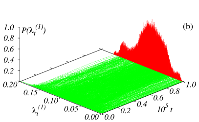
Figure 1: (Color online) Local FTLEs as a function of time for $N=4$, showing their dependence on $10^{3}$ distinct ICs. After the last iteration the FTLEs distribution over the ICs is plotted in red (for better visualization we used $10^{6}$ ICs.) In this example we used global coupling with (a) $K=1.0$ and (b) $K=0.21$.

For small values of $K$ a large amount of regular motion in phase space is expected and thus strong sticky motion. This can be observed, for example, in Fig. 1(b) for $K=0.21$. In such cases the FTLEs distribution is not Gaussian-like and it can be multimodal. This is a very complicated region to be characterized in general since only a tiny portion of ICs lead to chaotic motion, and these are responsible for the Arnold diffusion and produce Arnold stripes in the mixed plots ICs versus nonlinear parameter [21, 18].

For the cases where the FTLE distribution is a Gaussian-like function, higher cummulants from this distribution are very efficient to detect tiny sticky motion, as was shown for the standard map [13] and for high-dimensional conservative systems [14]. Here we show results determining the skewness, or the asymmetry of the FTLEs distribution. The skewness is defined by $\kappa_{3}=\displaystyle{\left<(\lambda_{t}-\left<\lambda_{t}\right>)^{3}\right>}/{\tilde{\sigma}^{3/2}}$, where $\sigma=\tilde{\sigma}/\left<\lambda_{t}\right>^{2}$ is the relative variance and $\lambda_{t}$ is the local FTLE. For $\kappa_{3}=0$ we have the regular Gaussian distribution, expected for a chaotic system. Since sticky motion usually reduces the FTLEs the asymmetry of the distribution leads to $\kappa_{3}<0$. Thus for any $\kappa_{3}<0$ sticky motion is expected. The flatness (forth cummulant) could also be used instead the skewness, but results are similar. For more details we refer the readers to [14], where it was shown that the variance of the FTLEs distribution is not that efficient to detect sticky motion as the flatness and skewness.

4 Characterizing weak chaos

The transition from the integrable case ($K=0$) to the weakly chaotic one depends on the kind of coupling between sites. As mentioned in the introduction, in the weakly chaotic region everything is complicated [1]: the positions of the regular structures, their size distribution, the shapes of the structures boundaries and the penetration inside them due to higher dimensions. As demonstrated above, the method of higher cummulants of the FTLEs distribution is not appropriate for too small $K$ values, where the amount of regular motion in phase space is much larger than the chaotic one. In order to understand better the integrable to weakly chaotic transition we analyze FTLEs in mixed plots as an additional tool. Such plots are very useful to study bifurcation diagrams in conservative systems [22].

4.1 The global coupling

We start considering the case $N=4$ for which $8$ symmetric FTLEs exist, two of them are exactly zero due to the conservation of the total momentum. An interesting way to describe the complicated global dynamics dependence on initial conditions, and thus the sticky effect, is shown in the mixed plot $K\times p_{0}^{(2)}$ presented in Fig. 2(a). Other dynamical quantities ($p_{0}^{(i)}$, with $i=1,2,3,\ldots$ could also be used instead $p_{0}^{(2)}$). Colors are the largest FTLEs after $10^{4}$ iterations. Initial conditions are chosen on the invariant structure $P_{T}=0.0$ and $X_{CM}=\sum_{j=1}^{N}X_{0}^{(j)}=0.0$. This plot shows, as a function of $K$, which initial conditions generate zero or positive FTLEs.

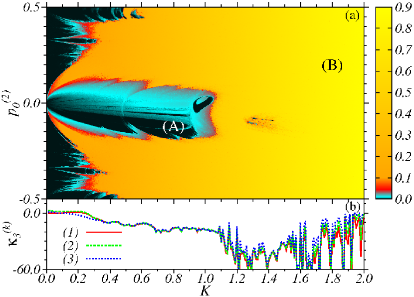
Figure 2: (Color online) Comparison of the (a) mixed plot $K\times p_{0}^{(2)}$ with the (b) skewness $\kappa_{3}^{(k)}$ for $N=4$ and the GC coupling (2). Continuous line for $k=1$, dashed for $k=2$ and dotted line for $k=3$.

A rich variety of structures is observed. Essentially two distinct larger regions of motions are observed and demarked in the plot as: (A) where FTLEs are smaller and (B) where FTLEs are larger. In between the FTLEs mix themselves along complicated and apparently fractal structures. For $K\to 0$ FTLEs go to zero inside region (A). However there are some stripes, which emanate from $K\sim 0$ for which FTLEs are larger. Two larger stripes are born close to $p_{0}^{(0)}\sim 0.0$ and growth symmetrically around this point as $K$ increases. Such stripes are intervals of initial conditions inside which Arnold diffusion occurs and are thus named as Arnold or Chaotic stripes. They exist for many intervals of initial conditions, as described in more details in [21, 18], where their apparency was also observed in open billiards with rounded corner/borders.

Along the line $p_{0}^{(2)}\sim 0.0$ the dynamics is almost regular for $K<1$, becoming chaotic for larger values of $K$. This picture shows us clearly that for the same $K$ value, different regions of the phase space (in this case $p_{0}^{(2)}$) have distinct FTLEs. Smaller FTLEs are related to those initial conditions which started exactly on a regular trajectory, or on a chaotic trajectory which touched for a finite time the regular structures from the high-dimensional phase space. Such regular structures can be global (as the invariant $P_{T}$), local, or collective ordered states which live in the high-dimensional phase space. As trajectories itinerate between ordered and random states, the regular structures affect locally the FTLEs inducing sticky motion, so that the corresponding FTLE decreases. Thus each point in the mixed plot from Fig. 2(a) which has smaller FTLEs for a fixed $K$ value, is necessarily related to sticky motion.

This is confirmed by comparing Fig. 2(a) and (b), where it is possible to associate stickiness $\kappa_{3}^{(k)}<0.0$ in Fig. 2(b) with the existence of initial conditions which generate close to zero FTLEs in Fig. 2(a). Figure 2(b) shows the skewness related to the distribution for the three remaining positive FTLEs as a function of $K$ for the GC. In this case $10^{4}$ random equally distributed initial conditions are used and $10^{6}$ iterations. For very small values of $K\lesssim 0.2$, we checked that the FTLEs distributions are not Gaussian-like, so that $\kappa_{3}^{(k)}$ is not well defined. For $K>0.2$ it can be seen in Fig. 2(b) that $\kappa_{3}^{(k)}\lesssim 0.0$ for all three FTLEs. Thus all FTLEs are equally affected by the regular structures leaving to sticky motion. Small changes between distinct $\kappa_{3}^{(k)}$ are observed close to $K\sim 2.0$ but since $\kappa_{3}^{(k)}\to 0.0$, no relevant sticky motion is expected to occur anymore and the dynamics can be characterized as totally chaotic for $K\gtrsim 2.0$.

We can identify a clear transition between three dynamical regions: strongly regular for $K\lesssim 0.3$, where $\kappa_{3}^{(k)}$ is probably not well defined and many initial conditions generate small FTLEs; strongly mixed for $0.3\lesssim K\lesssim 1.8$ where many sticky regions are observed $\kappa_{3}^{(k)}<0.0$ and; the chaotic one for $K\gtrsim 1.8$ where $\kappa_{3}^{(k)}\to 0.0$. Interesting to mention is that in the mixed region we observe the common motion, where all FTLEs are equally affected by the regular structures in the high-dimensional phase space.

To compare our results with the ordering states shown in [20], we firstly write down the order parameter

$$Z_{t}=\frac{1}{\sqrt{N}}\sum_{j=1}^{N}exp{\left[2\pi ix_{t}^{(j)}\right]}.$$ (8)

From this parameter it is possible to distinguish essentially three motions [20]: (i) when $Z_{t}=N$, i.e. all $x_{t}^{(j)}$ are the same; (ii) when $Z_{t}\approx 1$, i.e. the $x_{t}^{(j)}$ are randomly distributed and (iii) when $Z_{t}=0$ which occurs if $x_{t}^{(j)}$ are evenly spaced. States (i) and (iii) are denominated ordered states while (ii) a chaotic (or random) state. It is essential to recognize that $Z_{t}$ is a local quantity and changes in time, oscillating between ordered and random states. In this sense, it is not so powerful to make general statements about the dynamics as the FTLEs distribution. Independent of that, it is interesting to look at the order parameter in the mixed plot $K\times p_{0}^{(2)}$, which gives us a clear picture of the dynamics dependence on the ICs. This is shown in Fig. 3 where the colors represent

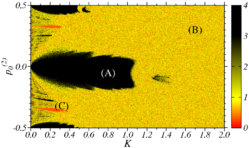
Figure 3: (Color online) Order parameter (see colors) shown for the mixed plot $K\times p_{0}^{(2)}$ for $N=4,t=10^{4}$, for the GC.

the order parameter. ICs are along the conservative quantity $P_{T}=0$ with center of mass $X_{CM}=0$. It is possible to distinguish three main regions: (A) where the order parameter $Z_{t}$ is close do $N=4$ (see color bar) meaning that a fully clustered motion is expected; (B) where $Z_{t}\sim 1.0$ and a random state is expected and (C) where $Z_{t}\sim 0.0$ and an ordered state is expected. The mixed plot very clearly relates the initial momentum in the phase space and the corresponding dynamics. Although the dynamics is well understood by such mixed plot, the order parameter has not a definitive value since this is a high-dimensional system and ordered and random states can alternate in time. To show the complexity of the dynamics in time, Fig. 4 shows a magnification of Fig. 3 for three different exemplary times: (a) $t=1.0\times 10^{3}$ (b) $t=9.0\times 10^{3}$, (c) $t=1.0\times 10^{4}$ and (d) FTLE for $t=1.0\times 10^{4}$.

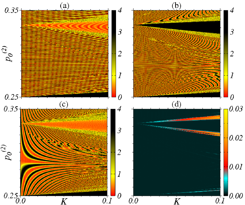
Figure 4: (Color online) Magnification from Fig. 3 (see white box) for four different times: (a) for $t=1.0\times 10^{3}$ (b) for $t=9.0\times 10^{3}$, (c) for $t=1.0\times 10^{4}$ and (d) FTLE.

Basically we identify three regions in Fig. 4(a): the large region with alternating values of $Z_{t}$ and two stripes, one red ($Z_{t}\sim 0.0$) and one black ($Z_{t}\sim 4.0$). These stripes increase as $K$ increases. However, as times goes on ($t=9.0\times 10^{3}$) Fig. 4(b) shows that inside the upper stripe the dynamics changes to a fully clustered state, while inside the lower stripe remains unchanged. As time increases to $t=1.1\times 10^{4}$ the dynamics inside the upper stripe changes again to $Z_{t}\sim 0.0$, showing the alternating dynamics between the two ordered states connected in time by the random state. The large region between the two stripes has now well defined structures which alternate in space between the two ordered states (black and red) connected by the random state (yellow), since we always observed this color between the ordered state. Figure 4(d) shows the corresponding FTLE which will be described below.

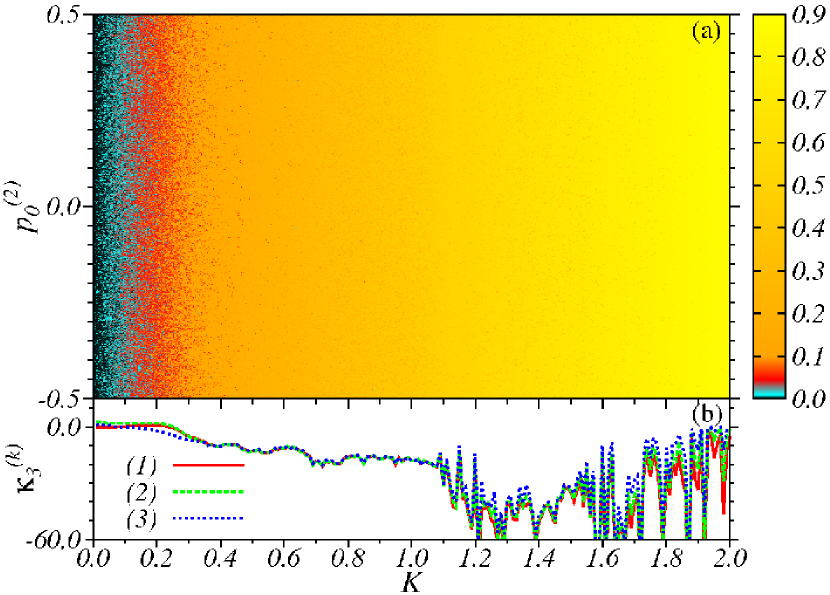
Figure 5: (Color online) The case of random ICs for (a) the mixed plot $K\times p_{0}^{(2)}$, (b) $\kappa_{3}^{k}$ and (c) the order parameter. Continuous line for $k=1$, dashed for $k=2$ and dotted line for $k=3$.

Comparing Figs. 2(a) and 3 it is possible to identify regions (A) and (B) showing an association between ordered state with small FTLEs and random states with larger FTLEs. This association however is not definitive since the order parameter, which defines the ordered and random states, may change in time. The distinction between the ordered state from regions (A) and (C) from Fig. 3 are not observed in Fig. 2(a). In fact, for smaller values of $K$ the dynamics is very rich and complicated. This is better observed in the magnifications shown in Fig. 4. While Figs. 4 (a)-(c) show the alternating dynamics of ordered states ($Z_{t}\sim 0.0\to 4.0\to 0.0\to\ldots$) inside the stripes mentioned above, Fig. 4(d) shows the FTLEs. Inside these stripes the FTLEs increase, meaning that the ordered states ($Z_{t}\sim 0.0,4.0$) present chaotic dynamics because they are connected through the random states which have ($Z_{t}\sim 1.0$). Outside the stripes the dynamics is very close to non-chaotic.

Although all figures and quantities discussed above nicely explain the dynamics, important changes occur when initial conditions are varied. For example, for the above discussed cases we always start initial conditions along the constant invariant structure $P_{T}=0$ and $X_{CM}=0$. By increasing the value of $P_{T}$ we observed (not shown) that region ($B$) and ($C$) from Figs. 3 and 2 start to decrease. This clearly means that when $P_{T}$ increases, the sticky time for which trajectories are trapped to invariant structures in phase space decreases. Moreless, the dynamics in the mixed plots changes drastically when initial conditions are chosen away from the invariant $P_{T}$. This is shown in Fig. 5(a) for the FTLEs. Initial conditions are chosen randomly. Very fast we recognize that almost only region (B) remains in the mixed plot. This agrees with the statements mentioned in [20], that as initial randomness increases the duration of ordered state decreases rapidly. On the other hand, the FTLEs shown in Fig. 5(a) already show that for small $K$ values the FTLEs decrease. But no stripes or well defined region with specific dynamics are observed. Clearly as $K$ increases, the amount of points related to sticky motion decreases and close to $K\sim 2.0$ only yellow points are observed, meaning that a strong chaotic behavior is expected. This is very easily confirmed by the $\kappa_{3}^{(k)}$, which tends to zero for $K\sim 2.0$. In distinction to the plot Fig. 5(a) the stickiness effect is accurately detected by $\kappa_{3}^{(k)}$ in Fig. 5(b).

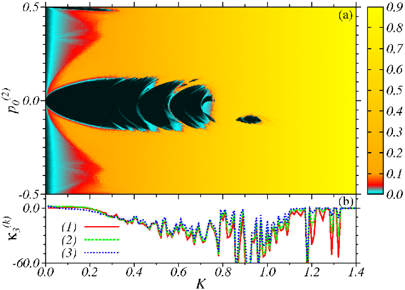
Figure 6: (Color online) Comparation of the (a) mixed plot $K\times p_{0}^{(2)}$ with the (b) skewness $\kappa_{3}^{(k)}$ for $N=4$ and the LC coupling (7). Continuous line for $k=1$, dashed for $k=2$ and dotted line for $k=3$.

Extensive numerical simulations were realized for values of $N=16$ and the main relevant observation is that for reasonable values of the nonlinear parameter $K\sim 0.10$, the dynamics is almost chaotic. For smaller values o $K\lesssim 0.03$ the regular portion of the phase space is so large that non-Gaussian FTLEs were found, making our method not appropriate for the analysis.

4.2 Local coupling

Now we continue to discuss the case $N=4$ but for the LC from Eq. (7). Figure 6(b) shows the skewness related to the distribution for the three positive FTLEs as a function of $K$. As for the GC numerical investigations, $10^{4}$ random equally distributed initial conditions are used and $10^{6}$ iterations. For values of $K\lesssim 0.2$ the FTLEs distributions are not Gaussian-like, so that $\kappa_{3}^{(k)}$ is not well defined. For $0.2\lesssim K\lesssim 1.1$ it can be seen in Fig. 6(b) that $\kappa_{3}^{(k)}<0.0$ for all three FTLEs. The FTLEs for the three unstable directions are almost equally affected by the regular structures leaving to sticky common motion. Tiny changes between distinct $\kappa_{3}^{(k)}$ are observed. For $K>1.1$, $\kappa_{3}^{(k)}\to 0.0$ but close to $K\sim 1.2,1.3$ we see effects of sticky motion. Figure 6(a) presents the mixed plot $K\times p_{0}^{(2)}$, where colors are the largest FTLEs after $10^{5}$ iterations. As in Fig. 2(a), initial conditions are chosen on the invariant structure $P_{T}=0.0$ and $X_{CM}=0.0$. Comparing with Fig. 2(a) we observe that the chaotic region and the sticky region close to $p_{0}^{(2)}$ remain almost unaltered. The essential differences occur for very small values of $K\lesssim 0.3$, where FTLEs are a small amount larger. Since we consider here the LC, the small perturbation in $K$ is not able to destroy the regular dynamics from the GC. In addition, the chaotic stripes observed Fig. 2(a) become blurred and the Arnold web is expected to be easier destroyed. By comparing Fig. 6(a) and (b), where again we can easily associate stickiness $\kappa_{3}^{(k)}<0.0$ in Fig. 6(b) with the existence of initial conditions which generate close to zero FTLEs in Fig. 6(a). The transition from strongly regular for $K\lesssim 0.2$, mixed for $0.3\lesssim K\lesssim 1.1$ and chaotic one for $K\gtrsim 1.1$ can be identified. For the particular values $K\sim 1.17,1.2,1.29,1.31$ the asymmetry $\kappa_{3}^{(k)}$ is negative in Fig. 6(b) and sticky motion should be present. Such points cannot be identified in Fig. 6(a), showing the power of the FTLEs distribution to detect the sticky motion.

For the case of random chosen ICs the chaotic stripes disappear and results are similar to those of Fig.5. In other words, the choice of ICs is also essential for the LC. Also for the LC we studied the case $N=16$ and results are almost similar to those from the GC.

5 Conclusions

The full characterization of the dynamics in high-dimensional Hamiltonian systems is a very difficult task. The restriction of plots to $2-$ and $3-$dimensions, the FTLEs dependence on initial conditions and sticky effects are the greater obstacles to solve this task for weakly chaotic systems. While the order parameter, studied extensively in [19, 20] for the coupled maps analyzed here, contains time dependent informations about dynamical states, the suitable quantities to fully characterize the dynamics are the higher order cummulants of the FTLEs distribution. In this work we only discuss results using the third cummulant, the skewness. Identical statements follow if one uses the forth cummulant, the kurtosis. The skewness gathers informations about ordered and random states and stickiness for each (un)stable directions from the phase space. In distinction to a previous work [14], here the characterization is performed to local and global couplings of $N=4$ maps in a conservative Hamiltonian system. Comparison with the order parameter were also realized. For very small perturbations the FTLEs distributions are not Gaussian-like and the skewness cannot be defined. For intermediate values of the perturbations the mixed dynamics was characterized for both, local and global couplings. It was observed that the common motion (i.e., that regular structures in phase space “attract” the chaotic trajectories by the same amount in all unstable directions) occurs independently of the coupling length. Additional numerical simulations have shown that the common motion tends to dissapear for a larger number of coupled maps and larger nonlinear parameter values. It was also shown that FTLEs shown in mixed plots (initial condition of the dynamical variable versus nonlinear parameter) are very convenient pictures to study the initial conditions dependence of the dynamics. Initial conditions which start inside invariant structures (total momentum $P_{T}=0$, in our case) tend to be regular for very long times, and sticky effects are of most importance. On the other hand, when initial conditions are chosen randomly, stickiness effects become less visible. These results also show the fundamental role of initial conditions in weakly chaotic systems.

References

References

- Chernikov et al. [1988] A.A. Chernikov, R.Z. Sagdeev, and G.M. Zaslavsky, Physics Today 41 (1988) 27.
- Meiss [1992] J.D. Meiss, Rev. Mod. Phys. 64 (1992) 795.
- Richter et al. [arXiv:1307.6109] M. Richter, S. Lange, A. Bäcker, and R. Ketzmerick (arXiv:1307.6109).
- Zaslavski [2002] G.M. Zaslavski, Phys. Rep. 371 (2002) 461.
- Livorati et al. [2012] A.L.P. Livorati, T. Kroetz, C.P. Dettmann, I.L. Caldas, E.D. Leonel, Phys. Rev. E 86 (2012) 036203.
- Pettini and Vulpiani [1984] M. Pettini and A. Vulpiani, Phys. Lett. 106A (1984) 207.
- K.Tsiganis et al. [2000] K. Tsiganis, A. Anastasiadis, and H. Varvoglis, Chaos, Solitons and Fractals 11 (2000) 2281.
- Malagoli et al. [1986] A. Malagoli, G. Paladin, and A. Vulpiani, Phys. Rev. A 34 (1986) 1550.
- Froyland and Padberg [2009] G. Froyland and K. Padberg, Physica D 238 (2009) 1507.
- Dellnitz and Junge [1997] M. Dellnitz and O. Junge, Int. J. Bif. and Chaos 7 (1997) 2475.
- Skokos et al. [2004] C. Skokos, C. Antonopoulos, T.C. Bountis, and M.N. Vrahatis, J. Phys. A 37 (2004) 6269.
- Antonopoulos et al. [2006] C. Antonopoulos, T. Bountis, and C. Skokos, Int. J. Bif. and Chaos 16 (2004) 1777.
- Tomsovic and Lakshminarayan [2007] S. Tomsovic and A. Lakshminarayan, Phys. Rev. E 76 (2007) 036207.
- C.Manchein et al. [2012] C. Manchein, M.W. Beims, and J.M. Rost, Chaos 22 (2012) 033137.
- Woellner et al. [2009] C.F. Woellner, S.R. Lopes, R.L. Viana, and I.L. Caldas, Chaos, Solitons and Fractals 41 (2009) 2201.
- K.Kaneko and T.Konishi [1989] K. Kaneko and T. Konishi, Phys. Rev. A 40 (1989) 6130.
- T.Konishi and K.Kaneko [1990] T. Konishi and K. Kaneko, J. Phys. A 23 (1990) 715.
- M.S.Custodio et al. [2012] M.S. Custodio, C. Manchein, and M.W. Beims, Chaos 22 (2012) 026112.
- T.Konishi and K.Kaneko [1992] T. Konishi and K. Kaneko, J. Phys. A 1992 (1992) 6283 .
- Kaneko and Konishi [1994] K. Kaneko and T. Konishi, Physica D 71 (1994) 146.
- Custodio and Beims [2011] M.S. Custodio and M.W. Beims, Phys. Rev. E 83 (2011) 056201.
- Manchein and Beims [2013] C. Manchein and M.W. Beims, Phys. Lett. A 377 (2013) 789.