On-shell constrained $M_{2}$ variables with applications to mass measurements and topology disambiguation

Abstract

We consider a class of on-shell constrained mass variables that are 3+1 dimensional generalizations of the Cambridge $M_{T2}$ variable and that automatically incorporate various assumptions about the underlying event topology. The presence of additional on-shell constraints causes their kinematic distributions to exhibit sharper endpoints than the usual $M_{T2}$ distribution. We study the mathematical properties of these new variables, e.g., the uniqueness of the solution selected by the minimization over the invisible particle 4-momenta. We then use this solution to reconstruct the masses of various particles along the decay chain. We propose several tests for validating the assumed event topology in missing energy events from new physics. The tests are able to determine: 1) whether the decays in the event are two-body or three-body, 2) if the decay is two-body, whether the intermediate resonances in the two decay chains are the same, and 3) the exact sequence in which the visible particles are emitted from each decay chain.

1 Introduction

The measurement of particle properties in events with missing energy at hadron colliders is a challenging problem which has been receiving increased attention as of late (see Barr:2010zj and Wang:2008sw for reviews on mass and spin measurement methods, respectively). The difficulty arises because in most new physics models with dark matter candidates, some conserved, often $Z_{2}$, parity is needed to make the dark matter stable. Particles which are charged with respect to this parity are pair produced; each such event contains at least two invisible (dark matter) particles whose energy and momenta are not measured. It is precisely this lack of information which makes the straightforward application of standard mass reconstruction techniques impossible.

In order to deal with the lack of knowledge about the invisible particle momenta, the following three approaches have been suggested:

• Use variables built from measured momenta only.

  The best known example is the invariant mass of (sets of) visible particles observed in the detector. The measurement of kinematic endpoints in various invariant mass distributions is the classic method for mass determination in supersymmetry  Hinchliffe:1996iu ; Bachacou:1999zb ; Allanach:2000kt ; Gjelsten:2004ki ; Gjelsten:2005aw ; Matchev:2009iw . Other recently proposed variables include the contransverse mass variable $M_{CT}$  Tovey:2008ui ; Polesello:2009rn and its variants $M_{CT_{\perp}}$ and $M_{CT_{\parallel}}$ Matchev:2009ad , the ratio of visible transverse energies Nojiri:2000wq ; Cheng:2011ya , and the energy itself Agashe:2012bn ; Agashe:2012fs ; Agashe:2013eba .

  Of course, while the individual invisible momenta are unknown, the sum of their transverse components is measured as the missing transverse momentum ${\;/\!\!\!\!\vec{P}_{T}}$ of the event. Thus one could also consider variables which are functions of the visible momenta and ${\;/\!\!\!\!\vec{P}_{T}}$, e.g., the transverse mass Smith:1983aa ; Barger:1983wf , the effective mass $M_{eff}$ Hinchliffe:1996iu ; Tovey:2000wk , the minimum partonic center-of-mass energy $\sqrt{\hat{s}}_{min}$ Konar:2008ei ; Konar:2010ma ; Robens:2011zm , the razor variables Rogan:2010kb ; Buckley:2013kua , etc. Such variables provide a good global characterization of the event, and are useful for discriminating signal from background, measuring an overall scale, or determining a signal rate. However, since they are not very sensitive to the particular details of the event, they are far from ideal for the purposes of precision studies of the signal.

• Calculate exactly the unknown individual momenta of the invisible particles.

  This is generally done by assuming a specific event topology and imposing a sufficient number of on-shell constraints Kawagoe:2004rz ; Nojiri:2007pq ; Cheng:2008mg ; Cheng:2009fw . If applicable, this method is very powerful, since the event kinematics is fully determined and one can easily move on to precision studies Cheng:2010yy . The main disadvantage of exact reconstruction techniques is that they require sufficiently long decay chains in order to provide the required number of mass-shell constraints. Otherwise, the system is underconstrained, and mass measurements are only possible on a statistical basis, by testing for consistency over the whole ensemble of signal events Cheng:2007xv ; Cheng:2008hk .

• Use a compromise approach.

  The third approach is a compromise between the previous two — one still constructs kinematic variables which depend on the invisible momenta, but one gives up on trying to determine those momenta exactly on an event-per-event basis. Instead, some kind of ansatz is used to assign values (consistent with the measured ${\;/\!\!\!\!\vec{P}_{T}}$) to the individual momenta of the invisible particles in each event. The most celebrated variable of this class is the Cambridge $M_{T2}$ variable Lester:1999tx ; Barr:2003rg , which is calculated by fixing the transverse momenta of the invisible particles to minimize the resulting transverse mass of the (larger of the two) parent particles. The idea of fixing the unknown invisible momenta by minimizing a suitable mass function is very powerful, and many of the kinematic variables proposed in the literature can be reinterpreted that way Barr:2011xt . The $M_{T2}$ approach is very well developed by now — analytical formulas exist for the calculation of $M_{T2}$ in a given event and for the interpretation of its endpoint Cho:2007qv ; Gripaios:2007is ; Barr:2007hy ; Cho:2007dh ; Burns:2008va ; Lester:2011nj ; Mahbubani:2012kx . Since the original $M_{T2}$ proposal Lester:1999tx ; Barr:2003rg , several other related variables have been suggested as well, e.g. $M_{T2\perp}$ and $M_{T2\parallel}$ Konar:2009wn , the asymmetric $M_{T2}$ Barr:2009jv ; Konar:2009qr , $M_{CT2}$ Cho:2009ve ; Cho:2010vz , and $M_{T2}^{approx}$ Lally:2012uj .

  Note that the $M_{T2}$ prescription determines only the transverse components of the invisible momenta. In order to fix the longitudinal components, one could rely on additional measurements or assumptions. For example, in the $M_{T2}$-assisted on-shell (MAOS) reconstruction method, one uses the measured $M_{T2}$ kinematic endpoint and enforces the on-shell condition for the mother particle, which allows one to solve for the longitudinal momenta Cho:2008tj ; Park:2011uz . (The idea behind the $M_{2C}$ variable Ross:2007rm ; Barr:2008ba is very similar.) A variation of this method arises if the invisible particles are neutrinos from $W$ (or $\tau$) decays — then one can use the known $W$-boson (or $\tau$-lepton) mass as a constraint and again solve for the longitudinal momenta Choi:2009hn ; Choi:2010dw ; Barr:2011he ; Barr:2011ux ; Barr:2011si ; Guadagnoli:2013xia . Since the on-shell constraints are nonlinear functions, the MAOS approach typically yields multiple solutions for the longitudinal momentum components, so one must also specify a prescription for handling this multiplicity.

  An alternative approach to MAOS, which may avoid this ambiguity, was outlined in Ref. Barr:2011xt , which pointed out that the $M_{T2}$ variable and its friends allow a 3+1 dimensional formulation, in which one always deals with the actual instead of the transverse masses. The corresponding 3+1 dimensional analogue of $M_{T2}$ was denoted simply as $M_{2}$, omitting the transverse index. The actual mass, being 3+1 dimensional, already carries dependence on both transverse and longitudinal momentum components, thus the minimization procedure required to obtain $M_{2}$ is expected to automatically assign unique values for all momentum components of each individual invisible particle. Since much of our discussion below will make crucial use of this property, we will discuss carefully the minimization procedure for the different $M_{2}$-type variables and the uniqueness of the resulting solutions for the invisible momenta in Sec. 3.

An important benefit from extending the transverse $M_{T2}$ formalism to the 3+1-dimensional $M_{2}$ language was recently emphasized in Mahbubani:2012kx . In many practical applications of $M_{T2}$ and similar kinematic variables, one has in mind a very specific signal topology, which in turn implies additional kinematic constraints on the (unknown) individual invisible momenta. For example, SUSY decay chains often proceed through intermediate on-shell resonances, the classic example being the decay of a heavy gluino through a lighter on-shell intermediate squark. While the mass of the intermediate resonance is a priori unknown, in symmetric event topologies the two decay chains are identical, so one may still impose the condition that the mass of the intermediate resonance (whatever its value) ends up being equal in the two decay chains Mahbubani:2012kx (for specific applications to $H\to\tau^{+}\tau^{-}$ and $H\to WW$ decay, see Barr:2011he and Barr:2011si , respectively). Adding such on-shell constraints further restricts the allowed domain of values for the components of the individual invisible momenta and in general leads to a different outcome from the minimization procedure, resulting in a new set of kinematic variables.

In this paper we shall extend the discussion from Mahbubani:2012kx , which focused only on intermediate resonances, i.e., particles appearing in the decay chain in between the decaying parent and the corresponding daughter. In particular, we shall allow ourselves to also consider resonances which appear “outside” the parent-daughter system, e.g., progenitor particles upstream from the parents, or descendant particles downstream from the daughters. The benefits from this generalization will become clear in the physics examples studied below.

In the paper, we study the mathematical properties of these on-shell constrained $M_{2}$ kinematic variables and propose several novel techniques for mass measurements and for disambiguating alternative event topologies. Our main results are:

• We find that differential distributions of the constrained $M_{2}$ variables exhibit sharper kinematic endpoints, making them easier to measure in the presence of backgrounds.

  This is because, as expected, the addition of on-shell kinematic constraints generally increases the value of the corresponding $M_{2}$ variable, thus providing a more stringent lower bound on the mass of the parent. The sharper endpoints would ultimately lead to an improvement in the precision with which the parent masses can be determined experimentally.

• We propose a new method for measuring the mass of a heavy resonance in a SUSY decay chain, by using the invisible momenta found during the $M_{2}$ minimization.

  The standard procedure so far has been to treat that resonance as a parent particle in a suitably defined subsystem of the event Burns:2008va , then measure the upper kinematic endpoint of the corresponding $M_{T2}$ distribution. Instead, here we treat the resonance as an on-shell constraint to be applied during the minimization process while calculating the $M_{2}$ variable for a suitably defined subsystem (which may or may not extend over the resonance itself). Since the $M_{2}$ minimization procedure selects a unique configuration for the individual invisible momenta, one has all the information required to reconstruct the mass of this hypothetical resonance directly. The key observation, supported in our examples in Sec. 4.2 below, is that the peak of that mass distribution is very well correlated with the true mass of the resonance. The spirit of our method is similar to MAOS reconstruction Cho:2008tj ; Choi:2009hn ; Choi:2010dw ; Park:2011uz ; Choi:2011ys ; Guadagnoli:2013xia and the $M_{2C}$ approach Ross:2007rm . The difference is that we do not rely on preliminary measurements of kinematic endpoints; the measurement is instead done from first principles.

• We find that this new method, in combination with other standard techniques, can be used to determine the mass of the invisible (dark matter) particles.

  An interesting feature of the method just described is that the result exhibits a different functional dependence on the test daughter mass than the results from analogous methods based on $M_{T2}$ or invariant mass kinematic endpoints. This means that one is able to obtain the true daughter mass by simply putting together the functional parent-daughter mass relationship obtained from our method and from the other canonical methods in the literature — the true answer is given by the crossing point of the different curves. This technique is complementary to the $M_{T2}$ “kink” method where one looks for a kink instead of a crossing point Cho:2007qv ; Gripaios:2007is ; Barr:2007hy ; Cho:2007dh ; Barr:2009jv (other techniques for measuring the absolute daughter mass are described in Matchev:2009ad ; Matchev:2009fh ; Alwall:2009sv ; Konar:2009wn ; Cohen:2010wv ).

• We propose methods for identifying the event topology and resolving combinatorial ambiguities.

  The large variety of on-shell constrained $M_{2}$ variables allows us to address a long standing problem in SUSY phenomenology, namely, the question of identifying the correct event topology. There are two aspects of the problem — first, resolving the combinatorial ambiguities in assigning the observed final state particles to the hypothesized event topology Rajaraman:2010hy ; Baringer:2011nh ; Choi:2011ys , and second, validation of the hypothesized event topology itself, e.g., the partitioning into two decay chains Bai:2010hd ; Cho:2012er , the number of invisible particles Agashe:2010gt ; Agashe:2010tu ; Giudice:2011ib ; Cho:2012er , the number of intermediate on-shell resonances Bai:2010hd ; Cho:2012er , etc. We can use the fact that the different versions of our on-shell constrained $M_{2}$ variables have different assumptions about the underlying event topology built in. Thus, by comparing results obtained with different $M_{2}$ variables, we can test those assumptions, for example:

  1. In Sec. 5.1 we design a method which tests for the presence of intermediate on-shell resonances in the SUSY decay chain, i.e., distinguishes between a sequence of two 2-body decays and a single 3-body decay.

  2. In Sec. 5.2 we address the question of the proper sequence in which the visible particles get emitted along a SUSY decay chain. We use the invisible particle momenta selected by the $M_{2}$ minimization procedure to construct Dalitz-type plots involving invariant masses of suitable particle pairs. The correct ordering of the visible particle is then determined by comparing the characteristic shapes of those plots.

  3. A similar idea, illustrated in Sec. 5.3, can be used to test whether the events are symmetric, i.e., whether the two decay chains are the same Konar:2009qr .

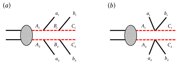
Figure 1: The decay topologies under consideration in this paper. In diagram (a), each parent particle, $A_{i}$, ($i=1,2$) decays to two visible particles, $a_{i}$ and $b_{i}$, and an invisible daughter particle, $C_{i}$, through an intermediate on-shell resonance, $B_{i}$. In diagram (b), the intermediate state, $B_{i}$, is absent (or very heavy) and the $A_{i}\to a_{i}b_{i}C_{i}$ decay is a three body process.

The paper is organized as follows. In Sec. 2, we specify the process studied (depicted in Fig. 1) and introduce our conventions and terminology. We then proceed to define all possible on-shell constrained $M_{2}$ variables for that process (a total of 12 variables altogether, listed in Table 2). However, not all of those variables are independent — Sec. 3 discusses the existing relationships among them, including the connection to the Cambridge $M_{T2}$ variable. The subsequent sections demonstrate the utility of those variables for practical applications: mass measurements from kinematic endpoints (Sec. 4.1), mass measurements from $M_{2}$-assisted peak reconstruction (Sec. 4.2), and topology disambiguation (Sec. 5). Sec. 6 is reserved for our conclusions.

2 Notations and setup

2.1 The physics process

In this paper we shall consider the generic processes depicted in Fig. 1. We assume the pair production of two heavy particles, $A_{1}$ and $A_{2}$, which decay in a similar fashion:

$$A_{i}\to a_{i}b_{i}C_{i},\quad(i=1,2).$$ (1)

The process (1) may occur either through on-shell intermediate resonances, $B_{i}$, as in Fig. 1(a), or as a genuine three-body decay, as in Fig. 1(b). The particles, $C_{i}$, are invisible in the detector — in realistic models, their role is typically played by some dark matter candidate, e.g., the lightest supersymmetric particle (LSP) in supersymmetry. The particles, $a_{i}$ and $b_{i}$, are SM particles which are visible in the detector, thus their 4-momenta $p_{a_{1}}^{\mu}$, $p_{b_{1}}^{\mu}$, $p_{a_{2}}^{\mu}$, and $p_{b_{2}}^{\mu}$ are measured known quantities. In contrast, the 4-momenta of the $C_{i}$, which we shall denote by $q_{i}^{\mu}$, are a priori unknown, and are only constrained by the ${\;/\!\!\!\!\vec{P}_{T}}$ measurement:

$$\vec{q}_{1T}+\vec{q}_{2T}={\;/\!\!\!\!\vec{P}_{T}}.$$ (2)

The masses of the particles along the red dashed lines in Fig. 1 are denoted by $m_{A_{1}}$, $m_{B_{1}}$, $\cdots$, $m_{C_{2}}$. The process (1) depicted in Fig. 1 covers a large class of physically interesting and motivated scenarios, including dilepton events from top pair production and decay, stop decays in supersymmetry ($\tilde{t}\to b\ell\tilde{\nu}_{\ell}$), and many more.

In what follows, we shall assume that all four visible particles $a_{i}$ and $b_{i}$ in Fig. 1 are distinguishable. As already mentioned in the introduction, depending on the nature of the visible particles $a_{i}$ and $b_{i}$, various combinatorial issues may arise, e.g.:

1. Should the four visible particles be partitioned as $2+2$, $1+3$, or $0+4$? This question can be answered relatively easily by studying suitable invariant mass distributions of the visible particles Bai:2010hd .

2. Another question is, which visible particles belong to the first decay chain ($a_{1}$, $b_{1}$) and which belong to the second ($a_{2}$, $b_{2}$). Two possible approaches have been pursued: first, by applying suitable cuts, one could try to increase the chances of picking the correct pairwise assignment Rajaraman:2010hy ; Baringer:2011nh ; Choi:2011ys . Alternatively, one could consider all possible assignments and then try to subtract out the contributions from wrong assignments (e.g., by the mixed event subtraction technique Hinchliffe:1996iu ).

3. Finally, when $a_{i}$ is distinguishable from $b_{i}$, one could also ask which of these two particles was emitted first and which came second. The answer to this question will be the subject of Sec. 5.2.

2.2 $M_{2}$ subsystems and the particle family tree

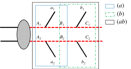
Figure 2: The decay process from Fig. 1(a) with the corresponding subsystems explicitly delineated. The blue dotted, green dot-dashed, and black solid lines indicate the subsystems $(a)$, $(b)$, and $(ab)$, respectively.

As first discussed in the context of the $M_{T2}$ variable Burns:2008va , one can proliferate the number of useful measurements by considering different subsystems within the original event. The subsystems are defined by the sets of visible particles which are used to construct an $M_{T2}$ variable (see Fig. 2):

• The $(ab)$ subsystem, indicated by the solid black box in Fig. 2. Here one uses both types of visible particles, $a_{i}$ and $b_{i}$, treating $A_{i}$ as parent particles and $C_{i}$ as daughter particles.

• The $(a)$ subsystem, shown by the blue dotted box in Fig. 2. Now one uses only the visible particles, $a_{i}$, but not $b_{i}$. The $A_{i}$ particles are again treated as parents, but the daughters are now the $B_{i}$ particles.

• The $(b)$ subsystem, depicted by the green dot-dashed box in Fig. 2. Now the visible particles, $b_{i}$, are used, but not $a_{i}$. The parents are the $B_{i}$ particles and the daughters are the $C_{i}$ particles.

In this paper, the $M_{T2}$ variables corresponding to these three subsystems will be denoted as $M_{T2}(ab)$, $M_{T2}(a)$, and $M_{T2}(b)$; the same convention will be used for the $M_{2}$ variables defined below.

We see that, depending on our choice of subsystem, each particle from Fig. 1(a) can be classified into one of the following three categories (summarized also in Table 1):

Subsystem	Parents $P_{i}$	Daughters $D_{i}$	Relatives $R_{i}$
$(ab)$	$A_{i}$	$C_{i}$	$B_{i}$
$(a)$	$A_{i}$	$B_{i}$	$C_{i}$
$(b)$	$B_{i}$	$C_{i}$	$A_{i}$

Table 1: The roles played by different particles depending on the subsystem under consideration.

• Parents. These are the two particles at the top of the decay chains in a given subsystem. In the following, we shall denote the parents by $P_{i},(i=1,2)$ and their masses by $M_{P_{i}}$. The $M_{2}$ kinematic variables in Sec. 2.3 below will be defined by a suitable minimization of the parent masses, $M_{P_{i}}$, over the unknown components of the invisible momenta Barr:2011xt .

• Daughters. These are the two particles at the end of the decay chains in a given subsystem. They may or may not be LSPs; see Table 1. The daughters will be denoted by $D_{i}$ and their masses by $M_{D_{i}}$. Each parent mass, $M_{P_{i}}$, is a function of the corresponding daughter mass, $M_{D_{i}}$, which is a priori unknown. Thus when calculating parent masses, one must always specify a test daughter mass parameter, which will be denoted by $\tilde{m}$ throughout this paper. For the most part, we shall be considering “symmetric” events, i.e., events in which the two decay chains are the same, and thus there is a single test mass $\tilde{m}$. The generalization to the asymmetric case is straightforward Konar:2009qr — one simply needs to introduce separate test masses, $\tilde{m}_{i}$, for the upper and the lower decay chains in Fig. 1.

• Relatives. These are particles which are neither parents nor daughters; see Table 1. The relatives will be denoted by $R_{i}$ and their masses by $M_{R_{i}}$. Since the decay chains in Fig. 1(a) involve only 3 new particles, there is always only one possible relative, which may appear upstream (as in the case of subsystem $(b)$), downstream (as in the case of subsystem $(a)$), or midstream (as in the case of subsystem $(ab)$). In other words, for the simple example of Fig. 1(a), the identity of the relative is uniquely fixed once we specify the subsystem under consideration, so we do not need to introduce any additional notation regarding the relatives. However, in more complicated examples with longer decay chains, there will be several relatives, and one would have to invent some notation to distinguish among them.

2.3 Definition of the on-shell constrained $M_{2}$ variables

We start by reviewing the standard definition of the canonical $M_{T2}$ variable Lester:1999tx . Consider the transverse masses $M_{TP_{i}}(\vec{q}_{iT},\tilde{m})$ of the two parent particles and then minimize the larger of them with respect to the transverse components of the invisible momenta, subject to the ${\;/\!\!\!\!\vec{P}_{T}}$ constraint, (2):

$$M_{T2}(\tilde{m}) \equiv \min_{\vec{q}_{1T},\vec{q}_{2T}}\left\{\max\left[M_{TP_{1}}(\vec{q}_{1T},\tilde{m}),\;M_{TP_{2}}(\vec{q}_{2T},\tilde{m})\right]\right\}.$$ (3)

$$\vec{q}_{1T}+\vec{q}_{2T} = {\;/\!\!\!\!\vec{P}_{T}}$$

Following Barr:2011xt , one could instead start with the actual parent masses, $M_{P_{i}}$, and define the 3+1-dimensional analogue of (3) as

$$M_{2}(\tilde{m}) \equiv \min_{\vec{q}_{1},\vec{q}_{2}}\left\{\max\left[M_{P_{1}}(\vec{q}_{1},\tilde{m}),\;M_{P_{2}}(\vec{q}_{2},\tilde{m})\right]\right\},$$ (4)

$$\vec{q}_{1T}+\vec{q}_{2T} = {\;/\!\!\!\!\vec{P}_{T}}$$

where the minimization is performed over the 3-component momentum vectors $\vec{q}_{1}$ and $\vec{q}_{2}$. As stated in Ross:2007rm ; Barr:2011xt , the two definitions (3) and (4) are equivalent, in the sense that the resulting two variables, $M_{T2}$ and $M_{2}$, will have the same numerical value (a proof of this claim can be found in Section 3.1 below). Nevertheless, for our purposes here, the definition (4) is much more convenient, for the following reasons:

• The minimization in (4) is done over the full 3-momentum vectors $\vec{q}_{1}$ and $\vec{q}_{2}$, and thus it also selects their longitudinal components $q_{1z}$ and $q_{2z}$. This completely fixes the kinematics of the event.

• The 3+1-dimensional language of Eq. (4) makes it very easy to impose the additional on-shell constraints that arise in specific event topologies Mahbubani:2012kx .

Given that here we are interested in the specific event topology of Fig. 1(a), it makes sense to consider additionally constrained versions of (4). There are two additional assumptions one can make: that the parents $P_{i}$ are the same (or, more generally, that they have the same mass)

$$M_{P_{1}}=M_{P_{2}},$$ (5)

or that the relatives have the same mass

$$M_{R_{1}}=M_{R_{2}}.$$ (6)

Of course, one could also impose (5) and (6) simultaneously, giving us a total of 4 possibilities. We choose to enumerate these 4 cases by adding two additional subscripts on the $M_{2}$ variable to indicate whether the constraints (5) and (6) were imposed during the minimization or not. The first subscript always refers to the parents and their constraint, (5), while the second subscript always refers to the relatives and their constraint, (6). The value of the subscript will be “C” if the corresponding constraint is imposed and “X” otherwise. Altogether, we have the following four types of variables:

$$M_{2XX} \equiv \min_{\vec{q}_{1},\vec{q}_{2}}\left\{\max\left[M_{P_{1}}(\vec{q}_{1},\tilde{m}),\;M_{P_{2}}(\vec{q}_{2},\tilde{m})\right]\right\},$$ (7)

$$\vec{q}_{1T}+\vec{q}_{2T} = {\;/\!\!\!\!\vec{P}_{T}}$$

$$M_{2CX} \equiv \min_{\vec{q}_{1},\vec{q}_{2}}\left\{\max\left[M_{P_{1}}(\vec{q}_{1},\tilde{m}),\;M_{P_{2}}(\vec{q}_{2},\tilde{m})\right]\right\},$$ (8)

$$\vec{q}_{1T}+\vec{q}_{2T} = {\;/\!\!\!\!\vec{P}_{T}}$$

$$M_{P_{1}} = M_{P_{2}}$$

$$M_{2XC} \equiv \min_{\vec{q}_{1},\vec{q}_{2}}\left\{\max\left[M_{P_{1}}(\vec{q}_{1},\tilde{m}),\;M_{P_{2}}(\vec{q}_{2},\tilde{m})\right]\right\},$$ (9)

$$\vec{q}_{1T}+\vec{q}_{2T} = {\;/\!\!\!\!\vec{P}_{T}}$$

$$M_{R_{1}}^{2} = M_{R_{2}}^{2}$$

$$M_{2CC} \equiv \min_{\vec{q}_{1},\vec{q}_{2}}\left\{\max\left[M_{P_{1}}(\vec{q}_{1},\tilde{m}),\;M_{P_{2}}(\vec{q}_{2},\tilde{m})\right]\right\}.$$ (10)

$$\vec{q}_{1T}+\vec{q}_{2T} = {\;/\!\!\!\!\vec{P}_{T}}$$

$$M_{P_{1}} = M_{P_{2}}$$

$$M_{R_{1}}^{2} = M_{R_{2}}^{2}$$

A few comments are in order. In the equations above, the masses of the parents, $M_{P_{i}}$, and the masses of the relatives, $M_{R_{i}}$, are always understood to be functions of the invisible 3-momenta $\vec{q}_{i}$. Thus the constraints $M_{P_{1}}=M_{P_{2}}$ and $M_{R_{1}}=M_{R_{2}}$ simply further restrict the allowed values for those momenta (in addition to the missing transverse momentum constraint, (2)). Obviously, the unrestricted variable $M_{2XX}$ is nothing but the variable defined in (4), so in this sense the pair of indices “XX” may seem redundant. Nevertheless, given the existence of the other three choices (8-10), it seems wise to indicate explicitly the absence of any on-shell constraints in that case.

We note that while a parent mass squared is always positive, there is one case when the mass squared of a relative can be negative — for subsystem $(a)$, the relative particle is $C_{i}$ and its mass squared is $M_{R_{i}}^{2}=(p_{B_{i}}-p_{b_{i}})^{2}$ (see Fig. 1(a)). Each of the 4-momenta $p_{B_{i}}^{\mu}$ and $p_{b_{i}}^{\mu}$ is time-like, but their difference may be time-like or space-like. Thus, in that situation, one has the option of additionally requiring positivity of the masses squared of relative particles. In this paper we shall not do that; we shall allow the relative masses squared obtained after the minimization to have either sign. This is why in Eqs. (9) and (10), the constraint for the relatives is written as $M_{R_{1}}^{2}=M_{R_{2}}^{2}$ instead of simply as $M_{R_{1}}=M_{R_{2}}$.

Subsystem $(ab)$		Subsystem $(a)$		Subsystem $(b)$
variable	constraints	variable	constraints	variable	constraints
$M_{2XX}(ab)$	–	$M_{2XX}(a)$	–	$M_{2XX}(b)$	–
$M_{2CX}(ab)$	$M_{A_{1}}^{2}=M_{A_{2}}^{2}$	$M_{2CX}(a)$	$M_{A_{1}}^{2}=M_{A_{2}}^{2}$	$M_{2CX}(b)$	$M_{B_{1}}^{2}=M_{B_{2}}^{2}$
$M_{2XC}(ab)$	$M_{B_{1}}^{2}=M_{B_{2}}^{2}$	$M_{2XC}(a)$	$M_{C_{1}}^{2}=M_{C_{2}}^{2}$	$M_{2XC}(b)$	$M_{A_{1}}^{2}=M_{A_{2}}^{2}$
$M_{2CC}(ab)$	$M_{A_{1}}^{2}=M_{A_{2}}^{2}$	$M_{2CC}(a)$	$M_{A_{1}}^{2}=M_{A_{2}}^{2}$	$M_{2CC}(b)$	$M_{B_{1}}^{2}=M_{B_{2}}^{2}$
	$M_{B_{1}}^{2}=M_{B_{2}}^{2}$		$M_{C_{1}}^{2}=M_{C_{2}}^{2}$		$M_{A_{1}}^{2}=M_{A_{2}}^{2}$

Table 2: A summary of the twelve $M_{2}$ variables defined in the text. For each of the three subsystems $(ab)$, $(a)$, and $(b)$, one may choose to apply neither, one, or both of the constraints (5) and (6). In each case, the trial daughter masses are assumed to be the same, $\tilde{m}$.

Applying (7-10) to the three possible subsystems of Fig. 2, we obtain a total of 12 on-shell constrained $M_{2}$ variables which are listed in Table 2. Some of these variables ($M_{2XX}$ and $M_{2CX}$) are simply 3+1 dimensional versions of $M_{T2}$ Barr:2011xt ; Mahbubani:2012kx , while $M_{2XC}(ab)$ and $M_{2CC}(ab)$ were mentioned in Mahbubani:2012kx . The remaining 4 variables $M_{2XC}(a)$, $M_{2CC}(a)$, $M_{2XC}(b)$, and $M_{2CC}(b)$ are new. Notice that the meaning of a “C” index depends on both its position (first or second) and on the chosen subsystem. For example, a “C” index sitting in first position, $M_{2CX}(ab)$, implies equality of the parents: $M_{A_{1}}^{2}=M_{A_{2}}^{2}$, while when sitting in second position, $M_{2XC}(ab)$, it indicates equality of the relatives: $M_{B_{1}}^{2}=M_{B_{2}}^{2}$. Similarly, contrast analogous variables in the three subsystems: $M_{2XC}(ab)$ is calculated assuming $M_{B_{1}}^{2}=M_{B_{2}}^{2}$; $M_{2XC}(a)$ is obtained with $M_{C_{1}}^{2}=M_{C_{2}}^{2}$; while $M_{2XC}(b)$ implies $M_{A_{1}}^{2}=M_{A_{2}}^{2}$.

At this point, it is instructive to consider a couple of specific examples, in order to better familiarize the reader with our notation. Consider, for example, $M_{2CC}(ab)$. It applies to the $(ab)$ subsystem, where $A_{i}$ are the parents, $C_{i}$ are the daughters (with test masses $\tilde{m}$) and $B_{i}$ are the relatives. Both indices are “on”, so the constraints (5) and (6) are applied. Explicitly, we have

$$M_{2CC}^{2}(ab) \equiv \min_{\vec{q}_{1},\vec{q}_{2}}\left\{\max\left[(p_{a_{1}}+p_{b_{1}}+q_{1})^{2},\;(p_{a_{2}}+p_{b_{2}}+q_{2})^{2}\right]\right\}.$$ (11)

$$q_{1}^{2} = \tilde{m}^{2}$$

$$q_{2}^{2} = \tilde{m}^{2}$$

$$\vec{q}_{1T}+\vec{q}_{2T} = {\;/\!\!\!\!\vec{P}_{T}}$$

$$(p_{a_{1}}+p_{b_{1}}+q_{1})^{2} = (p_{a_{2}}+p_{b_{2}}+q_{2})^{2}$$

$$(p_{b_{1}}+q_{1})^{2} = (p_{b_{2}}+q_{2})^{2}$$

As another example, consider $M_{2XC}(a)$. It applies to the $(a)$ subsystem with $A_{i}$ as parents, $B_{i}$ as daughters, and $C_{i}$ as relatives. Note that the test mass, $\tilde{m}$, now refers to $m_{B_{i}}$. The parents are not assumed to have equal masses, but the relatives are, thus

$$M_{2XC}^{2}(a) \equiv \min_{\vec{q}_{1},\vec{q}_{2}}\left\{\max\left[(p_{a_{1}}+p_{b_{1}}+q_{1})^{2},\;(p_{a_{2}}+p_{b_{2}}+q_{2})^{2}\right]\right\}.$$ (12)

$$(q_{1}+p_{b_{1}})^{2} = \tilde{m}^{2}$$

$$(q_{2}+p_{b_{2}})^{2} = \tilde{m}^{2}$$

$$\vec{q}_{1T}+\vec{q}_{2T} = {\;/\!\!\!\!\vec{P}_{T}}$$

$$q_{1}^{2} = q_{2}^{2}$$

Our final example is $M_{2XC}(b)$, which reads

$$M_{2XC}^{2}(b) \equiv \min_{\vec{q}_{1},\vec{q}_{2}}\left\{\max\left[(p_{b_{1}}+q_{1})^{2},\;(p_{b_{2}}+q_{2})^{2}\right]\right\}.$$ (13)

$$q_{1}^{2} = \tilde{m}^{2}$$

$$q_{2}^{2} = \tilde{m}^{2}$$

$$\vec{q}_{1T}+\vec{q}_{2T} = {\;/\!\!\!\!\vec{P}_{T}}$$

$$(p_{a_{1}}+p_{b_{1}}+q_{1})^{2} = (p_{a_{2}}+p_{b_{2}}+q_{2})^{2}$$

If it wasn’t for the very last constraint, this would have been simply $M_{T2}(b)$, i.e., the $M_{T2}$ variable for the $(b)$ subsystem, in the presence of upstream momentum $p_{a_{1}}+p_{a_{2}}$. However, the constraint for the relatives $M_{A_{1}}=M_{A_{2}}$ is non-trivial and leads to a qualitatively new result.

3 Relations among the $M_{2}$ type variables and $M_{T2}$

In this section, we examine the relations among the four $M_{2}$ type variables defined in the preceding section and compare them to the conventional $M_{T2}$ variable. For concreteness, we shall focus on the $(ab)$ subsystem and consider the set

$$M_{T2}(ab),\;\;\;M_{2XX}(ab),\;\;\;M_{2CX}(ab),\;\;\;M_{2XC}(ab),\;\;\;M_{2CC}(ab).$$ (14)

We shall perform our study under the assumption that the intermediate particles, $B_{i}$, are on-shell as in Fig. 1(a). The off-shell scenario of Fig. 1(b) will be discussed in Sec. 5 in the context of applications. In Sec. 3.1, we first show that the three variables, $M_{2XX}(ab)$, $M_{2CX}(ab)$, and $M_{T2}(ab)$, have the same value event-by-event. Informed by this discussion, in Sec. 3.2, we shall also discuss the question of the uniqueness of the invisible momentum configurations found in the process of minimization. Then, in Sec. 3.3, we shall discuss the hierarchy among the three distinct variables on the list (14), namely $M_{2CX}(ab)$, $M_{2XC}(ab)$, and $M_{2CC}(ab)$. In Sec. 3.4, we summarize the main results from Sec. 3.

3.1 Equivalence theorem among $M_{2XX},\;M_{2CX}$, and $M_{T2}$

Applying the general definition (3) to the $(ab)$ subsystem, $M_{T2}(ab)$ can be expressed as follows Lester:1999tx :

$$M_{T2}^{2}(ab) = \min_{\vec{q}_{1T},\vec{q}_{2T}}\left\{\max\left[M_{TA_{1}}^{2}(\vec{q}_{1T},\tilde{m}),\;M_{TA_{2}}^{2}(\vec{q}_{2T},\tilde{m})\right]\right\}$$ (15)

$$\vec{q}_{1T}+\vec{q}_{2T} = {\;/\!\!\!\!\vec{P}_{T}}$$

where

$$M_{TA_{i}}^{2}(\vec{q}_{iT},\tilde{m})={\tilde{m}}^{2}+m_{v_{i}}^{2}+2\left[E_{v_{i}T}E_{q_{i}T}-\vec{p}_{v_{i}T}\cdot\vec{q}_{iT}\right],$$ (16)

$v_{i}$ is the visible state $a_{i}+b_{i}$ belonging to the $i$-th decay chain:

$$\vec{p}_{v_{i}}\equiv\vec{p}_{a_{i}}+\vec{p}_{b_{i}},$$ (17)

and $E_{T}$ denotes the transverse energy:

$$E_{v_{i}T}=\sqrt{m_{v_{i}}^{2}+\vec{p}_{v_{i}T}^{\,2}}\,;\qquad E_{q_{i}T}=\sqrt{{\tilde{m}}^{2}+\vec{q}_{iT}^{\,2}}.$$ (18)

Using (7), we can construct $M_{2XX}(ab)$ in a similar manner:

$$M_{2XX}^{2}(ab) = \min_{\stackrel{{\scriptstyle\vec{q}_{1T},\vec{q}_{2T}}}{{q_{1z},q_{2z}}}}\left\{\max\left[M_{A_{1}}^{2}(\vec{q}_{1T},q_{1z},\tilde{m}),\;M_{A_{2}}^{2}(\vec{q}_{2T},q_{2z},\tilde{m})\right]\right\}.$$ (19)

$$\vec{q}_{1T}+\vec{q}_{2T} = {\;/\!\!\!\!\vec{P}_{T}}$$

The invariant masses of $A_{1}$ and $A_{2}$ can be written as

$$M_{A_{i}}^{2}(\vec{q}_{iT},q_{iz},\tilde{m})={\tilde{m}}^{2}+m_{v_{i}}^{2}+2\left[E_{v_{i}T}E_{q_{i}T}\cosh(\Delta\eta_{i})-\vec{p}_{v_{i}T}\cdot\vec{q}_{iT}\right],$$ (20)

where $\Delta\eta_{i}$ is the rapidity difference between the visible state $v_{i}$ and particle $C_{i}$. The minimization of (19) over the transverse momenta, $\vec{q}_{iT}$, and the longitudinal momenta, $q_{iz}$, can in principle be done in any order, but it is much easier to minimize over $q_{iz}$ first, since they do not enter the ${\;/\!\!\!\!\vec{P}_{T}}$ constraint. Furthermore, the longitudinal momenta are decoupled from each other, and thus the two minimizations can be performed independently. We can therefore rewrite (19) as

$$M_{2XX}^{2}(ab) = \min_{\vec{q}_{1T},\vec{q}_{2T}}\left\{\max\left[\min_{q_{1z}}\left\{M_{A_{1}}^{2}(\vec{q}_{1T},q_{1z},\tilde{m})\right\},\;\min_{q_{2z}}\left\{M_{A_{2}}^{2}(\vec{q}_{2T},q_{2z},\tilde{m})\right\}\right]\right\}.~{}~{}~{}$$ (21)

$$\vec{q}_{1T}+\vec{q}_{2T} = {\;/\!\!\!\!\vec{P}_{T}}$$

where we have switched the order of the $\min_{q_{iz}}\{\}$ and $\max\{\}$ operations. The minimization over $q_{iz}$ is equivalent to minimization over $\Delta\eta_{i}$. From (20) it is easy to see that the minimum is obtained for $\Delta\eta_{i}=0$, which reduces (20) to (16), so that (21) becomes simply

$$M_{2XX}^{2}(ab) = \min_{\vec{q}_{1T},\vec{q}_{2T}}\left\{\max\left[M_{TA_{1}}^{2}(\vec{q}_{1T},\tilde{m}),\;M_{TA_{2}}^{2}(\vec{q}_{2T},\tilde{m})\right]\right\}.~{}~{}~{}$$ (22)

$$\vec{q}_{1T}+\vec{q}_{2T} = {\;/\!\!\!\!\vec{P}_{T}}$$

Comparing (22) with (15), we see that Barr:2011xt

$$M_{2XX}^{2}(ab)=M_{T2}^{2}(ab).$$ (23)

Moving our attention to $M_{2CX}(ab)$, we see that the proof of its equivalence to $M_{T2}(ab)$ is not difficult either. A formal proof based on the method of Lagrange multipliers is presented in Appendix A, so here we shall give just the heuristic argument.

Starting from Eq. (23), without any loss of generality we can assume that $M_{2XX}^{2}(ab)$ is obtained by minimizing $M_{A_{1}}^{2}$, i.e., that in the neighborhood of the minimum, we have $M_{A_{2}}^{2}<M_{A_{1}}^{2}$, and thus the $\max$ function in the definition (19) picks up $M_{A_{1}}^{2}$ for the minimization. The parent constraint $M_{A_{1}}=M_{A_{2}}$ is clearly not satisfied, but this can be fixed without changing the value obtained in Eq. (23). Keeping $\vec{q}_{1T}$, $q_{1z}$, and $\vec{q}_{2T}$ fixed to their values at the $M_{2XX}^{2}(ab)$ minimum, we start varying $q_{2z}$ in the direction of increasing $M_{A_{2}}$. Eventually, we will find a value for $q_{2z}$ for which $M_{A_{2}}$ will reach $M_{A_{1}}$ and the parent constraint $M_{A_{1}}=M_{A_{2}}$ will be satisfied. In the meantime, nothing has changed regarding the $M_{A_{1}}^{2}$ function: since $\vec{q}_{1T}$ and $q_{1z}$ were kept the same as before, its value is still given by (23).

This simple exercise shows that by adjusting the longitudinal invisible momenta, one can always turn $M_{2XX}$ into $M_{2CX}$:

$$M_{2CX}^{2}(ab)=M_{2XX}^{2}(ab).$$ (24)

The main lesson is that this comes at a price — the invisible momentum configuration selected by the $M_{2XX}$ minimization may be different from the configuration obtained in the $M_{2CX}$ minimization. We shall have much more to say about this in Sec. 3.2 below.

Combining (24) with (23), we also trivially obtain the relation Mahbubani:2012kx

$$M_{2CX}^{2}(ab)=M_{T2}^{2}(ab).$$ (25)

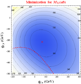
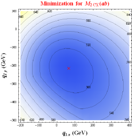
Figure 3: Contour plots of the functions $f_{T2}(\vec{q}_{1T})$ (left panel), $f_{2XX}(\vec{q}_{1T})$ (middle panel), and $f_{2CX}(\vec{q}_{1T})$ (right panel) in the plane of $\vec{q}_{1T}$. The chosen event leads to an unbalanced solution for $M_{T2}(ab)$. (The red dashed curve delineates the points with $M_{TA_{1}}=M_{TA_{2}}$.) The red $\times$ symbol marks the global minimum of the function in each case. At the minimum, $M_{T2}(ab)=M_{2XX}(ab)=M_{2CX}(ab)=483.71$ GeV, and the corresponding solution for $\vec{q}_{1T}$ is given by $\vec{q}_{1T}^{\,\times}=(66.09,-212.90)$ GeV.

In order to illustrate (23-25) pictorially, in Fig. 3 we plot the three functions

$$f_{T2}(\vec{q}_{1T}) \equiv \max\left[M_{TA_{1}}(\vec{q}_{1T},\tilde{m}),\;M_{TA_{2}}({\;/\!\!\!\!\vec{P}_{T}}-\vec{q}_{1T},\tilde{m})\right],$$ (26)

$$f_{2XX}(\vec{q}_{1T}) \equiv \min_{q_{1z},q_{2z}}\left\{\max\left[M_{A_{1}}(\vec{q}_{1T},q_{1z},\tilde{m}),\;M_{A_{2}}({\;/\!\!\!\!\vec{P}_{T}}-\vec{q}_{1T},q_{2z},\tilde{m})\right]\right\},$$ (27)

$$f_{2CX}(\vec{q}_{1T}) \equiv \min_{\stackrel{{\scriptstyle q_{1z},q_{2z}}}{{M_{A_{1}}=M_{A_{2}}}}}\left\{\max\left[M_{A_{1}}(\vec{q}_{1T},q_{1z},\tilde{m}),\;M_{A_{2}}({\;/\!\!\!\!\vec{P}_{T}}-\vec{q}_{1T},q_{2z},\tilde{m})\right]\right\}$$ (28)

in the $\vec{q}_{1T}$ plane. ($\vec{q}_{2T}$ is then determined from the ${\;/\!\!\!\!\vec{P}_{T}}$ constraint as $\vec{q}_{2T}={\;/\!\!\!\!\vec{P}_{T}}-\vec{q}_{1T}$.) These are precisely the functions which need to be minimized over $\vec{q}_{1T}$ in order to obtain the variables $M_{T2}(ab)$, $M_{2XX}(ab)$, and $M_{2CX}(ab)$, respectively. Note that these functions already contain different number of minimizations over longitudinal momenta: $f_{2XX}(\vec{q}_{1T})$ has two, $f_{2CX}(\vec{q}_{1T})$ has one (the other longitudinal degree of freedom is fixed by the $M_{A_{1}}=M_{A_{2}}$ constraint), while $f_{T2}(\vec{q}_{1T})$ has none. The event chosen for Fig. 3 was selected such that the associated $M_{T2}(ab)$ value comes from an unbalanced situation, i.e., the minimum of $f_{T2}(\vec{q}_{1T})$, marked with the red $\times$ symbol, is at $M_{TA_{1}}\neq M_{TA_{2}}$.

Fig. 3 demonstrates that the three functions (26-28) are identical, thus justifying the identities (23-25). In other words, once the minimization over the longitudinal components is done for the $M_{2XX}(ab)$ and $M_{2CX}(ab)$ variables, the remaining functions $f_{2XX}(\vec{q}_{1T})$ and $f_{2CX}(\vec{q}_{1T})$ become identical to $f_{T2}(\vec{q}_{1T})$, so the remaining minimization over $\vec{q}_{1T}$ will converge to the common point marked with the $\times$ symbol. This means that all three variables $M_{2XX}(ab)$, $M_{2CX}(ab)$, and $M_{T2}(ab)$ not only have a common value, but also select the same transverse components $\vec{q}_{iT}$ for the invisible momenta at their respective minima. However, this is not the case for the longitudinal invisible momenta, $q_{iz}$, which will be the subject of the next subsection.

3.2 Uniqueness of the longitudinal momenta found by $M_{2XX}$ and $M_{2CX}$

As already mentioned in the Introduction, one of the main advantages of the $M_{2}$-type variables over purely transverse analogues like $M_{T2}$, $M_{CT2}$ etc., is that they supply values for not just the transverse, but also the longitudinal components of the invisible particle momenta. The knowledge of the full 4-momentum of each invisible particle enables us to reconstruct the mass of each particle along the decay chain, and in particular the relative particles; see Sec. 4.2. One should keep in mind that the momenta found by the $M_{2}$ minimization are not the actual momenta of the invisible particles in the event. Nevertheless, the MAOS approach demonstrates that they can be successfully used for reconstruction Cho:2008tj ; Park:2011uz ; Guadagnoli:2013xia .

Let us now investigate the solutions for $q_{1z}$ and $q_{2z}$ more closely. Consider the starting point of the $M_{2XX}$ calculation, the function

$$G_{2XX}(\vec{q}_{1T},q_{1z},q_{2z})\equiv\max\left[M_{A_{1}}(\vec{q}_{1T},q_{1z},\tilde{m}),\;M_{A_{2}}({\;/\!\!\!\!\vec{P}_{T}}-\vec{q}_{1T},q_{2z},\tilde{m})\right].$$ (29)

As we saw in Sec. 3.1, its minimization along the transverse directions $\vec{q}_{1T}$ results in unique solutions; we call them $\vec{q}_{1T}^{\,(\times)}$. (See the red $\times$ symbols in Fig. 3). Therefore, for the purposes of discussing the minimization over the longitudinal momentum components, we can fix the transverse momenta, $\vec{q}_{1T}=\vec{q}_{1T}^{\,(\times)}$, and investigate the $q_{iz}$ dependence of the function

$$g_{2XX}(q_{1z},q_{2z}) \equiv \max\left[M_{A_{1}}(\vec{q}_{1T}^{\,(\times)},q_{1z},\tilde{m}),\;M_{A_{2}}({\;/\!\!\!\!\vec{P}_{T}}-\vec{q}_{1T}^{\,(\times)},q_{2z},\tilde{m})\right].$$ (30)

The unconstrained minimization of $g_{2XX}(q_{1z},q_{2z})$ over $q_{1z}$ and $q_{2z}$ yields the value of $M_{2XX}$, while minimizing (30) subject to the parent constraint, $M_{A_{1}}=M_{A_{2}}$, gives the value of $M_{2CX}$.

Let us first study the effect of the parent constraint

$$(p_{a_{1}}+p_{b_{1}}+q_{1})^{2}=(p_{a_{2}}+p_{b_{2}}+q_{2})^{2},$$ (31)

which can be solved for $q_{2z}$ in terms of $q_{1z}$:

$$q_{2z}=\frac{p_{v_{2}z}K\pm E_{v_{2}}\sqrt{K^{2}-E_{q_{2}T}^{2}(E_{v_{2}}^{2}-p_{v_{2}z}^{2})}}{E_{v_{2}}^{2}-p_{v_{2}z}^{2}},$$ (32)

where

$$K\equiv\frac{m_{v_{1}}^{2}-m_{v_{2}}^{2}}{2}+E_{q_{1}}E_{v_{1}}-\vec{q}_{1T}\cdot\vec{p}_{v_{1}T}-q_{1z}p_{v_{1}z}+\vec{q}_{2T}\cdot\vec{p}_{v_{2}T}.$$ (33)

One can obtain an analogous expression for $q_{1z}$ in terms of $q_{2z}$, by substituting $v_{1}\leftrightarrow v_{2}$ and $q_{1}\leftrightarrow q_{2}$ in Eqs. (32) and (33).

A couple of observations can be made from these equations. First, one can easily see from (32) that the $q_{2z}$ solution is not uniquely determined, i.e., $q_{2z}$ has a twofold ambiguity for a fixed $q_{1z}$, unless the expression inside the square root, the discriminant, vanishes. The same argument can be made regarding the analogous expression giving $q_{1z}$ in terms of $q_{2z}$. Then the question becomes whether both $q_{1z}$ and $q_{2z}$ have double roots for some $\vec{q}_{1T}$. This is where the second observation comes into play. It turns out that for the value of $q_{1z}$ which minimizes the function (29), $q_{1z}^{\,(min)}$, the discriminant in Eq. (32) is proportional to the difference between the transverse masses of $A_{1}$ and $A_{2}$:

$$\left.K^{2}-E_{q_{2}T}^{2}(E_{v_{2}}^{2}-p_{v_{2}z}^{2})\right|_{q_{1z}^{\,(min)}}\propto\left(M_{TA_{1}}^{2}-M_{TA_{2}}^{2}\right).$$ (34)

On the other hand, the discriminant that would appear in the expression analogous to (32) giving $q_{1z}$ in terms of $q_{2z}$, will be proportional to $M_{TA_{2}}^{2}-M_{TA_{1}}^{2}$, i.e., the difference of the same squared transverse masses, only taken in opposite order. This suggests an interesting complementarity, in which $q_{1z}$ and $q_{2z}$ do not suffer from twofold ambiguities simultaneously, i.e., if $q_{2z}$ has two solutions in Eq. (32), then $q_{1z}$ is uniquely determined, and vice versa. This observation also reveals the necessary condition for both $q_{1z}$ and $q_{2z}$ to be uniquely determined simultaneously: the transverse masses of $A_{1}$ and $A_{2}$ must be the same, $M_{TA_{1}}=M_{TA_{2}}$, see the red dashed curves in Fig. 3.

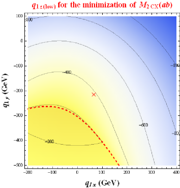
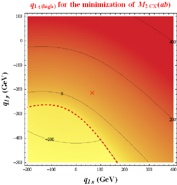
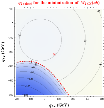
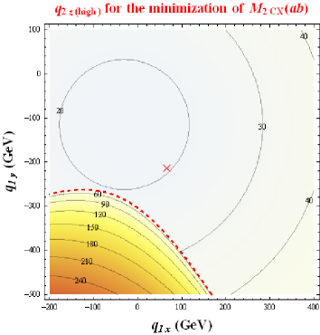
Figure 4: The values of the longitudinal invisible momenta $q_{iz(low)}$ (left panels) and $q_{iz(high)}$ (right panels) which solve the parent constraint, (31), in the $\vec{q}_{1T}$ plane ($\vec{q}_{2T}$ is then given by the ${\;/\!\!\!\!\vec{P}_{T}}$ condition (2)), for the same event shown in Fig. 3. The upper row shows $q_{1z(low)}$ and $q_{1z(high)}$ for $q_{2z}=q_{2z}^{\,(min)}$, while the lower row shows $q_{2z(low)}$ and $q_{2z(high)}$ for $q_{1z}=q_{1z}^{\,(min)}$. ($q_{iz}^{\,(min)}$ is always found by minimizing (29).) The red dashed curves denote the contours where the solutions to both $q_{1z}$ and $q_{2z}$ are unique.

Fig. 4, which was made for the same unbalanced event used in Fig. 3, pictorially illustrates the above discussion. Let us call the two solutions of (32) $q_{2z(low)}$ (corresponding to the “$-$” sign) and $q_{2z(high)}$ (corresponding to the “$+$” sign). They are plotted in the lower two panels of Fig. 4 in the $\vec{q}_{1T}$ plane. The remaining momenta are fixed as follows: at each point of the plane, $\vec{q}_{2T}$ is given by the ${\;/\!\!\!\!\vec{P}_{T}}$ condition (2), while $q_{1z}$ is chosen so that it minimizes the function (29): $q_{1z}=q_{1z}^{\,(min)}$. The upper two panels of Fig. 4 show the analogous plots where the roles of $q_{1z}$ and $q_{2z}$ are reversed — we find $q_{2z}$ by minimizing (29), $q_{2z}=q_{2z}^{\,(min)}$, and then plot the two solutions for $q_{1z}$, $q_{1z(low)}$ and $q_{1z(high)}$. The red dashed lines delineate the points with balanced solutions for $M_{T2}$, $M_{TA_{1}}=M_{TA_{2}}$.

Fig. 4 confirms that the red dashed line is a watershed boundary — in the region above and to the right of that line we always find two possible values for $q_{1z}$, but a single value for $q_{2z}$. Conversely, in the area below and to the left of that line there is always a unique solution for $q_{1z}$, but two solutions for $q_{2z}$ instead. Now recall that the event depicted in Figs. 3 and 4 was unbalanced, i.e., the true global minimum was obtained at the red $\times$ point, at which $M_{TA_{1}}\neq M_{TA_{2}}$. This point also happens to be located in the region where the solution for $q_{2z}$ is unique, but the solution for $q_{1z}$ has a twofold ambiguity. On the other hand, if we had chosen a balanced event, the global minimum would fall somewhere on the red dashed line, and both $q_{1z}$ and $q_{2z}$ will be uniquely determined.

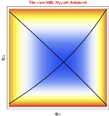
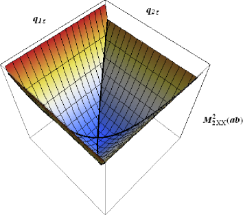
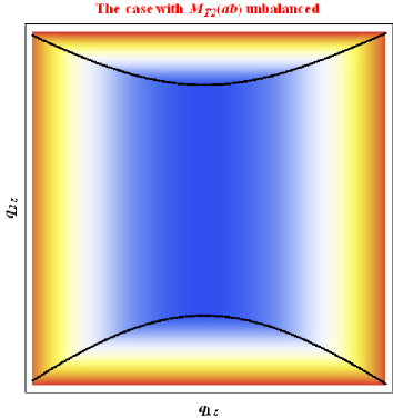
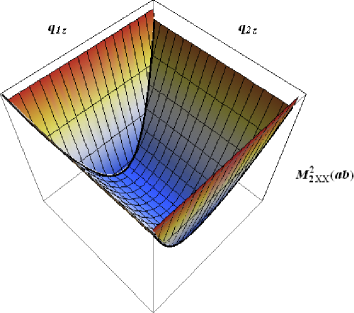
Figure 5: Plot of the function (30) in the $(q_{1z},q_{2z})$ plane, for a balanced event with $M_{TA_{1}}=M_{TA_{2}}$ at the minimum (top row) and an unbalanced event with $M_{TA_{1}}\neq M_{TA_{2}}$ at the minimum (bottom row). The left panels are contour plots, while the right panels show the corresponding 3-dimensional view. The black solid curves mark the points satisfying the parent constraint, $M_{A_{1}}=M_{A_{2}}$.

Having understood the minimization of $M_{2CX}(ab)$, it is easy to infer the corresponding solutions for $q_{1z}$ and $q_{2z}$ in the case of $M_{2XX}(ab)$. The ambiguity problem is now even more serious, because whenever $q_{iz(low)}\neq q_{iz(high)}$, any value of $q_{iz}\in\left(q_{iz(low)},q_{iz(high)}\right)$ is also allowed, i.e., the ambiguity is not just twofold, instead there is a flat direction. However, these ambiguities are present only for unbalanced events — for balanced events, $q_{iz(low)}=q_{iz(high)}$, and the solution for both $q_{1z}$ and $q_{2z}$ is unique. This is pictorially illustrated in Fig. 5, which shows the function (30) as a function of $q_{1z}$ and $q_{2z}$. Since $\vec{q}_{1T}$ is already fixed to its correct value, $\vec{q}_{1T}^{\,(\times)}$, at the global minimum of (29), the global unconstrained minimum of the function (30) seen in Fig. 5 corresponds to $M_{2XX}$, while the constrained minimization along the black solid lines with $M_{A_{1}}=M_{A_{2}}$ yields the value of $M_{2CX}$. The two plots in the top row of Fig. 5 correspond to a balanced event, in which there is a single global minimum, and thus the longitudinal momentum configuration at the minimum is unique. Furthermore, the global minimum is at the intersection of the two black solid lines, implying that the parent constraint, $M_{A_{1}}=M_{A_{2}}$, is satisfied and therefore $M_{2XX}=M_{2CX}$, in agreement with the theorem from Sec. 3.1. On the other hand, the bottom two plots show an unbalanced event, in which the unconstrained minimization reveals a flat direction along $q_{2z}$. Any value of $q_{2z}$ along the bottom of that valley is acceptable and will give the correct value of $M_{2XX}$. If we now consider the constrained minimization along the black solid lines to obtain $M_{2CX}$, we find two degenerate global minima — one on the upper black solid curve and one on the lower black solid curve. Thus, as expected, there is a twofold ambiguity — in this case in the value of $q_{2z}$, while $q_{1z}$ is unique. Again, the values of $M_{2XX}$ and $M_{2CX}$ are the same, since the function (30) is constant along the flat direction.

Since later on we shall be using the momenta found by the minimization for reconstruction purposes, the results from this subsection raise the question of how one should deal with unbalanced events, for which (some of) the momentum components are not uniquely determined. There can be several approaches:

• Restrict one’s attention to balanced events only, incurring some (minor) loss in statistical significance.

• Sum over all possible kinematic solutions (i.e., integrate over the flat direction in Fig. 5), and enter the results in histograms with correspondingly reduced weights.

• Instead of obtaining the momenta from $M_{2XX}$ and $M_{2CX}$, use the variables with relative constraints, $M_{2XC}$ and $M_{2CC}$, for which these ambiguities generally do not arise, see Sec. 3.3.

3.3 The variables $M_{2XC}$ and $M_{2CC}$

Having seen in Sec. 3.1 that $M_{2XX}(ab)$ and $M_{2CX}(ab)$ are equivalent to $M_{T2}(ab)$, we now shift our focus to the new variables $M_{2XC}(ab)$ and $M_{2CC}(ab)$ and investigate their relationship with the other variables.

First we argue that the result from minimization with respect to $\vec{q}_{1T}$ will be different in general when obtaining these new variables. For this purpose, let us assume the opposite, i.e., consider the function (30) in which $\vec{q}_{1T}$ has been fixed to the result $\vec{q}_{1T}^{\,(\times)}$ found in the $\vec{q}_{1T}$ minimization in Fig. 3. We then discuss its minimization in the $(q_{1z},q_{2z})$ plane as in Fig. 5. The new element here is the presence of the relative constraint, $M_{B_{1}}^{2}=M_{B_{2}}^{2}$, which can be written as

$$(p_{b_{1}}+q_{1})^{2}=(p_{b_{2}}+q_{2})^{2},$$ (35)

and which can be solved for $q_{2z}$ in analogy to (32):

$$q_{2z}=\frac{p_{b_{2}z}K^{\prime}\pm E_{b_{2}}\sqrt{K^{{}^{\prime}2}-E_{q_{2}T}^{2}p_{b_{2}T}^{2}}}{p_{b_{2}T}^{2}},$$ (36)

where

$$K^{\prime}\equiv E_{q_{1}}E_{b_{1}}-\vec{q}_{1T}\cdot\vec{p}_{b_{1}T}-q_{1z}p_{b_{1}z}+\vec{q}_{2T}\cdot\vec{p}_{b_{2}T}.$$ (37)

A similar expression can be obtained for $q_{1z}$ in terms of $q_{2z}$, with the replacements $q_{2z}\leftrightarrow q_{1z}$ and $b_{1}\leftrightarrow b_{2}$ in (36,37). Due to the “$\pm$” sign in (36), the relative constraint, (35), again implies two branches in the $(q_{1z},q_{2z})$ plane, analogous to the black solid curves in Fig. 5. If at least one of these two curves passes through the global minimum point found previously for the case of $M_{2XX}$, then $M_{2XC}$ will turn out to be the same as $M_{2XX}(ab)$. However, the chances of a plane curve passing through a given point (or even a given finite line segment) are minimal, therefore we expect that, in general, the solution found previously for $M_{2XX}$ will not obey the relative constraint, (35). This means that our choice of $\vec{q}_{1T}=\vec{q}_{1T}^{\,(\times)}$ was wrong, and that the minimum for $M_{2XC}$ is obtained at a different value for $\vec{q}_{1T}$ than the one found in Fig. 3. In particular, the constrained global minimum found by $M_{2XC}$ will be higher than the corresponding unconstrained global minimum $M_{2XX}$:

$$M_{2XC}(ab)\geq M_{2XX}(ab)=M_{2CX}(ab)=M_{T2}(ab).$$ (38)

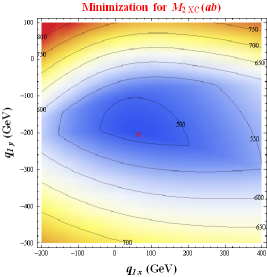
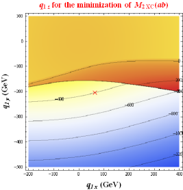
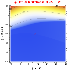
Figure 6: The analogues of Fig. 3 (left panel) and Fig. 4 (middle and right panels) for the case of $M_{2XC}$. The cross symbols show the location of the global minimum for $M_{XC}$, at which $M_{2XC}(ab)=483.85$ GeV, and the invisible momenta are given by $(\vec{q}_{1T},\;q_{1z},\;q_{2z})=(64.61,\;-202.37,\;-395.75,\;19.07)$ GeV.

Fig. 6 pictorially illustrates the above discussion. The left panel shows the function to be minimized when calculating $M_{2XC}$. As compared with the analogous Fig. 3 for the case of $M_{2XX}$, we see that the shape of the function is completely different, and as a result the global minimum (marked with a red $\times$ symbol) is obtained at a different point in $\vec{q}_{T}$ space, $\vec{q}_{1T}=(64.61,-202.37)$ GeV (as opposed to $\vec{q}_{1T}^{\,\times}=(66.09,-212.90)$ GeV, which was found in Fig. 3).

Another important lesson from the middle and right panels in Fig. 6 is that the solutions for $q_{1z}$ and $q_{2z}$ are now unique, unlike in the case of $M_{2XX}$ and $M_{2CX}$ exhibited in Fig. 4. We shall use this fact later on when reconstructing the mass of relative particles and studying the event topology.

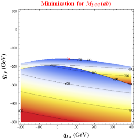
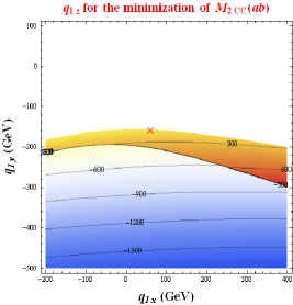
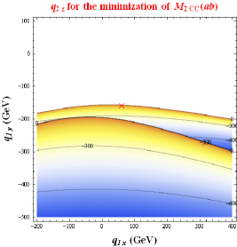
Figure 7: The same as Fig. 6, but for the case of $M_{2CC}(ab)$. At the global minimum (marked with the red $\times$ symbol), $M_{2CC}(ab)=487.86$ GeV, and the solution for the invisible momenta is given by $(\vec{q}_{1T},\;q_{1z},\;q_{2z})=(60.11,\;-156.62,\;121.35,\;17.44)$ GeV. Within the white region, the constraints (31) and (35) cannot be simultaneously satisfied.

Finally, it remains to discuss the variable $M_{2CC}(ab)$, where the parent and relative constraints, (31) and (35), are simultaneously applied. The analysis proceeds very similarly to the case of $M_{2XC}(ab)$ and the corresponding results are displayed in Fig. 7. Because of the additional constraint, the true global minimum for $M_{2CC}(ab)$ is now even greater than $M_{2XC}(ab)$. We thus arrive at our final result relating the variables (14):

$$M_{2CC}(ab)\geq M_{2XC}(ab)\geq M_{2XX}(ab)=M_{2CX}(ab)=M_{T2}(ab).$$ (39)

Note that there are large regions in invisible momentum parameter space (the white areas in Fig. 7), for which the on-shell kinematic constraints (31) and (35) cannot be simultaneously satisfied. As before, the red $\times$ symbol marks the solution for $\vec{q}_{1T}$, which is found at a new location, $\vec{q}_{1T}=(60.11,-156.62)$ GeV. The corresponding $M_{2CC}(ab)$ value is $487.86$ GeV, which is slightly larger than $M_{2XC}(ab)=483.85$ GeV, in agreement with (39). The solutions for the longitudinal momenta are also unique (just as in the case of $M_{2XC}(ab)$ in Fig. 6), and are found at $(q_{1z},q_{2z})=(121.35,17.44)$ GeV.

3.4 Summary of the properties of the on-shell constrained $M_{2}$ variables

We now collect our main results from Sec. 2 and Sec. 3 before moving on to the practical applications of the $M_{2}$ variables in the next few sections.

In Sec. 2, we defined five different types of variables for each of the three subsystems in Fig. 2 (see Table 2). The hierarchy among those variables is

$$M_{2CC}(ab)\geq M_{2XC}(ab)\geq M_{2XX}(ab)=M_{2CX}(ab)=M_{T2}(ab);$$ (40)

$$M_{2CC}(a)\geq M_{2XC}(a)\geq M_{2XX}(a)=M_{2CX}(a)=M_{T2}(a);$$ (41)

$$M_{2CC}(b)\geq M_{2XC}(b)\geq M_{2XX}(b)=M_{2CX}(b)=M_{T2}(b).$$ (42)

Thus, out of the fifteen variables seen in (40-42), there are only nine which are quantitatively different.

	Balanced events		Unbalanced events
Variable	$\vec{q}_{iT}$	$q_{iz}$	$\vec{q}_{iT}$	$q_{iz}$
$M_{T2}(ab)$	unique	NA	unique	NA
$M_{2XX}(ab)$	unique	unique	unique	flat direction
$M_{2CX}(ab)$	unique	unique	unique	twofold ambiguity
$M_{2XC}(ab)$	unique	unique	unique	unique
$M_{2CC}(ab)$	unique	unique	unique	unique

Table 3: Table summarizing the uniqueness of the invisible momentum configurations corresponding to the global minimum.

Each of the $M_{2}$ variables in Table 2 is calculated by minimizing a suitably defined mass function in terms of the invisible momenta, see (7-10). The global minimum thus selects a special configuration of the invisible momenta which can be used for kinematical studies. In this section, we also investigated the uniqueness of the global minimum and consequently, the uniqueness of the associated invisible momenta. Our results are summarized in Table 3. For completeness, in the table we also include the $M_{T2}$ variable, which, however, cannot determine the longitudinal components of the invisible momenta. In the case of balanced events, all four $M_{2}$ variables uniquely determine the invisible 3-momenta, while for unbalanced events, only $M_{2XC}$ and $M_{2CC}$ do so. Note that the twofold ambiguity in the case of $M_{2CX}$ and the flat direction in the case of $M_{2XX}$ are only with respect to one of the $q_{iz}$ components, while the other $q_{iz}$ component is uniquely determined.

4 Mass measurements

We now discuss several physics examples illustrating the potential uses and advantages of the $M_{2}$ variables. In this section, we first consider the simpler scenario where we have made the correct hypothesis about the true physics model and show how the use of $M_{2}$ variables can improve the precision of the mass measurements (in Sec. 4.1) and provide a generalization of the MAOS technique Cho:2008tj (in Sec. 4.2). Then in Sec. 5, we move to the case where we are uncertain about which new physics model is correct. We show how one can then use the $M_{2}$ variables to rule out the incorrect model assumptions and hone in on the correct event topology.

The model to be studied in this section is the one depicted in Fig. 1(a), where the two decay chains are assumed to be identical:

$$m_{A_{1}}=m_{A_{2}}\equiv m_{A},\;\;\;m_{B_{1}}=m_{B_{2}}\equiv m_{B},\;\;\;m_{C_{1}}=m_{C_{2}}\equiv m_{C}.$$ (43)

In order to avoid confusion, from here on we shall use lowercase letters as in (43) to denote the true physical masses of the particles, reserving the corresponding uppercase letters $M_{A}$, $M_{B}$, etc., for masses which are reconstructed using kinematic information from the visible decay products in the event. Where necessary, input test masses (i.e., mass ansätze) will be denoted with a tilde. Throughout the paper, for our simulations we shall use event samples of $\sim 100,000$ events each, generated at threshold ($\sqrt{\hat{s}}=m_{A_{1}}+m_{A_{2}}$) without any spin correlations (i.e. we use pure “phase space” distributions).

4.1 $M_{2}$ kinematic endpoints and parent mass measurements

The relations (40-42) imply that the on-shell constrained variables $M_{2XC}$ and $M_{2CC}$ can provide progressively better measurements of an upper kinematic endpoint, as compared with the conventional variables $M_{T2}$, $M_{2XX}$, and $M_{2CX}$. The reason is that the shapes of the $M_{2XC}$ and $M_{2CC}$ distributions will be skewed to the right, thus better populating the bins in the vicinity of the endpoint.

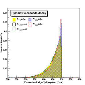
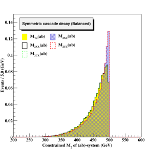
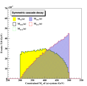
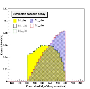
Figure 8: Unit-normalized differential distributions of the variables $M_{T2}$ (yellow shaded histograms), $M_{2XX}$ (black solid line), $M_{2CX}$ (green dashed line), $M_{2XC}$ (blue hatched histograms), and $M_{2CC}$ (red dashed line) for the process of Fig. 1(a) with mass spectrum $(m_{A},\;m_{B},\;m_{C})=(500,\;300,\;200)$ GeV. Results are shown for subsystem $(ab)$ (upper left panel), subsystem $(ab)$ with balanced events only (upper right panel), subsystem $(a)$ (lower left panel), and subsystem $(b)$ (lower right panel). The input trial mass is chosen to be the same as the true mass of the relevant daughter particle.

This expectation is confirmed in Fig. 8, where we compare the distributions of these five variables for the example of (43) with mass spectrum $(m_{A},\;m_{B},\;m_{C})=(500,\;300,\;200)$ GeV. For concreteness and simplicity, we choose the input trial mass, $\tilde{m}$, to be the same as the actual daughter mass in each case. Comparisons are made for each subsystem of Fig. 2: subsystem $(ab)$ (upper left panel), subsystem $(ab)$ but using only balanced events (upper right panel), subsystem $(a)$ (lower left panel), and subsystem $(b)$ (lower right panel). Although each panel shows results for five variables, only three distributions (at most) can be seen, because the distributions of $M_{T2}$, $M_{2XX}$, and $M_{2CX}$ are identical, in accordance with the equivalence theorem from Sec. 3.1. An interesting observation is that $M_{2CC}$ and $M_{2CX}$ also turn out to be the same for balanced events (i.e., events in which the transverse masses of the parents end up being equal for the momentum configuration obtained when minimizing the respective mass function). This observation is supported by the upper right plot in Fig. 8, which uses only events in which $M_{T2}(ab)$ is obtained from a balanced configuration, and by the two lower plots in Fig. 8, in which $M_{T2}(a)$ and $M_{T2}(b)$ always come from balanced configurations.

In the case of subsystem $(ab)$, the $M_{T2}$ distribution is already very sharp near the kinematic endpoint, and the improvement from replacing $M_{T2}$ with $M_{2XC}$ or $M_{2CC}$ appears marginal. However, the effect is very drastic in the case of subsystem $(a)$ or subsystem $(b)$ (the lower two plots in Fig. 8), where the $M_{T2}$ distribution (the yellow-shaded histogram) has very few events near the kinematic endpoint. Now, using $M_{2XC}$ or $M_{2CC}$ in place of $M_{T2}$ completely changes the character of the distribution, and the bins near the endpoint become the most populated ones. Notice the extremely sharp drop-off at the endpoint of the $M_{2XC}(a)$ and $M_{2XC}(b)$ distributions (the blue-shaded histograms). This feature should be easily observable over the background and would lead to more accurate endpoint measurements and extraction of masses.

4.2 $M_{2}$-assisted mass reconstruction of relative peaks

As explained in the introduction, an attractive feature of the $M_{T2}$ variable is that it provides an ansatz for the transverse momenta of the invisible particles. The $M_{2}$ variables, being 3+1 dimensional extensions of $M_{T2}$, take this one step further and extend the ansatz to the full 4-momenta of the invisible particles. This allows us to apply the MAOS method for mass reconstruction Cho:2008tj ; Choi:2009hn ; Choi:2010dw in a pure form, i.e., without the need for additional assumptions in order to solve for the longitudinal momenta of the invisible particles — since those are already provided by the $M_{2}$ minimization itself. As shown in Sec. 3, the variables $M_{2CC}$ and $M_{2XC}$ are somewhat better suited for our purpose (in comparison to $M_{2XX}$ and $M_{2CX}$), since they provide a unique ansatz for the invisible particle momenta in the case of unbalanced events. Of course, for balanced events, any of our four types of $M_{2}$ variables can be used.

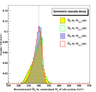
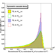
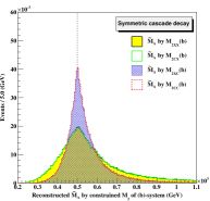
Figure 9: Reconstruction of the mass of the relative particle in the case of subsystem $(ab)$ (left panel), subsystem $(a)$ (middle panel), and subsystem $(b)$ (right panel). The ansatz for the invisible particle momenta can be taken from the corresponding $M_{2XX}$ variable (yellow-shaded histogram), $M_{2CX}$ variable (green histogram), $M_{2XC}$ variable (blue-shaded histogram), or $M_{2CC}$ variable (red histogram). The true mass spectrum and trial masses are chosen as in Fig. 8. The vertical black dashed line in each plot denotes the true mass of the associated relative particle. The middle panel (for subsystem $(a)$) shows the mass squared of the relative particle, which can be negative at times.

Fig. 9 shows the results for the reconstruction of the masses of the relative particles in each of the three subsystems from Fig. 2. In the left panel of Fig. 9, we use the invisible momenta obtained from various $M_{2}(ab)$-type variables to reconstruct the mass, $\tilde{M}_{B}$, of the relative particle, $B$, in subsystem $(ab)$; in the middle panel we use the momenta obtained from $M_{2}(a)$-type variables to find the mass squared, $\tilde{M}_{C}^{2}$, of the relative particle, $C$, in subsystem $(a)$; and finally, in the right panel, we use the momenta from $M_{2}(b)$-type variables to reconstruct the mass, $\tilde{M}_{A}$, of the relative particle, $A$, in subsystem $(b)$. Each distribution in Fig. 9 is color coded according to the type of $M_{2}$ variable supplying the invisible momenta: yellow-shaded histograms for the case of $M_{2XX}$, green histograms for $M_{2CX}$, blue-shaded histogram for $M_{2XC}$, and red histograms for $M_{2CC}$. The events are generated with the mass spectrum from Eq. (43) and the test mass was always chosen to be the true mass of the relevant daughter particle: $\tilde{m}=m_{C}$ for subsystem $(ab)$ (left panel), $\tilde{m}=m_{B}$ for subsystem $(a)$ (middle panel), and $\tilde{m}=m_{C}$ for subsystem $(b)$ (right panel).

The most interesting feature of the plots in Fig. 9 is that the distributions always peak close to the true mass of the relative particle (denoted by the vertical black dashed line in each plot). This suggests a new technique for measuring the mass of a relative particle — by using the location of the peak of the reconstructed relative mass distribution as shown in Fig. 9. A closer inspection of Fig. 9 reveals another advantage of the $M_{2}$ variables that incorporate on-shell kinematic constraints for relative particles in their definition. Note that in each panel, all four distributions peak near the true relative mass, but in the case of $M_{2XC}$ and (especially) $M_{2CC}$, the peak is much more narrow, and, more importantly, the peak location is very close to the true value of the mass of the respective relative particle. We therefore anticipate that the precision of the new technique will be much better when using $M_{2CC}$ (and $M_{2XC}$) as opposed to $M_{2CX}$ or $M_{2XX}$.

This technique is in principle independent of (and complementary to) the previous methods in which masses are measured from upper kinematic endpoints. For example, consider particle $B$ (the intermediate particle in the decay chains of Fig. 1). It is known that its mass can be measured (as a function of $\tilde{m}\equiv\tilde{m}_{C}$) from the upper kinematic endpoint $M_{T2}^{max}(b)$ of the $M_{T2}(b)$ distribution in subsystem $b$, where $B_{i}$ is treated as a parent Barr:2003rg ; Burns:2008va

$$\tilde{m}_{B}(\tilde{m}_{C})=M_{T2}^{max}(b)(\tilde{m}_{C}).$$ (44)

Using the correct value for the daughter particle mass, $m_{C}$, in (44) yields the correct value of the parent mass, $m_{B}$:

$$m_{B}=M_{T2}^{max}(b)(m_{C}).$$ (45)

We now propose to consider subsystem $(ab)$ instead, where $B_{i}$ is treated as a relative, and extract $\tilde{m}_{B}(\tilde{m}_{C})$ from the location of the peak $\tilde{M}_{B}^{peak}$ of one of the $\tilde{M}_{B}$ distributions in the left panel of Fig. 9, e.g., the one where the invisible momenta are fixed by $M_{2CC}(ab)$:

$$\tilde{m}_{B}(\tilde{m}_{C})=\tilde{M}_{B}^{peak}(ab)(\tilde{m}_{C}).$$ (46)

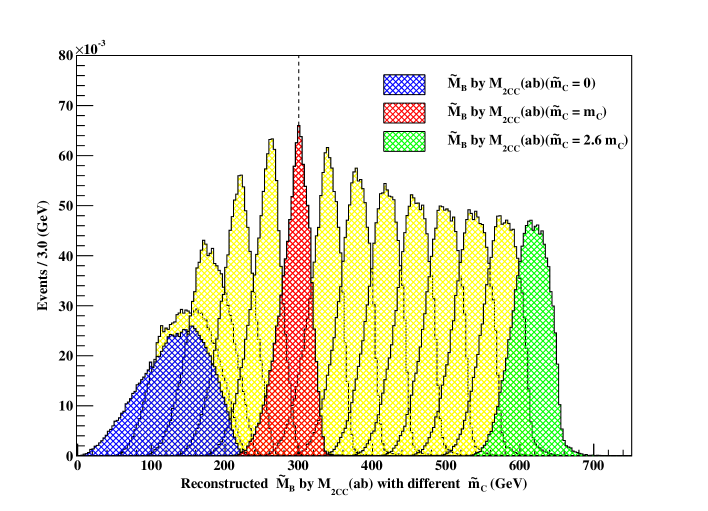
Figure 10: Unit-normalized distributions of the reconstructed mass, $\tilde{M}_{B}$, of the relative particle in subsystem $(ab)$, using invisible momenta from $M_{2CC}(ab)$, and picking a series of different values for the input test mass, $\tilde{m}_{C}$, from $\tilde{m}_{C}=0$ (blue histogram) to $\tilde{m}_{C}=2.6m_{C}$ (green histogram). The red shaded distribution corresponds to the true value, $\tilde{m}_{C}=m_{C}$, and is the same as the red histogram in the left panel of Fig. 9. The vertical black dashed line marks the true mass, $m_{B}=300$ GeV, in our example.

The procedure is pictorially illustrated in Fig. 10. The $\tilde{M}_{B}$ distribution from Fig. 9 can now be re-obtained without the “cheat” of fixing $\tilde{m}=m_{C}$. Instead, we can now simply vary the input test mass, $\tilde{m}_{C}$, and read off the location of the $\tilde{M}_{B}$ peak for each $\tilde{m}_{C}$ value, thus experimentally determining the function (46). This method relies on the fact demonstrated by the red shaded histogram in Fig. 10 — that for the correct value, $m_{C}$, of the test daughter mass the peak of the $\tilde{M}_{B}$ distribution matches the correct value, $m_{B}$, of the mass for the relative particle:

$$m_{B}=\tilde{M}_{B}^{peak}(ab)(m_{C}).$$ (47)

Notice the analogy between the relationships (44) and (46) — they both relate the mass of particle $B_{i}$ with the mass of particle $C_{i}$. The difference is that the correlation (44) is derived from a kinematic endpoint in subsystem $(b)$, while the correlation (46) is derived from the peak of a distribution within subsystem $(ab)$. Also one should keep in mind that while (45) is a mathematical identity, the relation (47) at this point is a conjecture supported by the numerical results from Figs. 9 and 10. (Compare to the similar conjecture relating the peak of the $\sqrt{\hat{s}}_{min}$ distribution to the mass of the corresponding parents Konar:2008ei .)

Similar logic can be applied to particle $A$. It is known that its mass can be measured from the upper kinematic endpoint of the $M_{T2}(ab)$ distribution in subsystem $(ab)$, as a function of the input test mass, $\tilde{m}_{C}$, in complete analogy to (44) Cho:2007qv ; Cho:2007dh :

$$\tilde{m}_{A}(\tilde{m}_{C})=M_{T2}^{max}(ab)(\tilde{m}_{C}).$$ (48)

Alternatively, it can be measured from the upper kinematic endpoint of the $M_{T2}(a)$ distribution in subsystem $(a)$, this time as a function of the test mass, $\tilde{m}_{B}$ Barr:2003rg ; Cho:2007dh ; Burns:2008va :

$$\tilde{m}_{A}(\tilde{m}_{B})=M_{T2}^{max}(a)(\tilde{m}_{B}).$$ (49)

We now propose a third way of measuring the mass of $A_{i}$, by treating it as a relative particle in subsystem $(b)$: using the invisible momenta from the $M_{2CC}(b)$ calculation, we can reconstruct the mass of the relative, $\tilde{M}_{A}$, and read off the location of the peak, $\tilde{M}_{A}^{peak}$, in analogy to (46)

$$\tilde{m}_{A}(\tilde{m}_{C})=\tilde{M}_{A}^{peak}(b)(\tilde{m}_{C}).$$ (50)

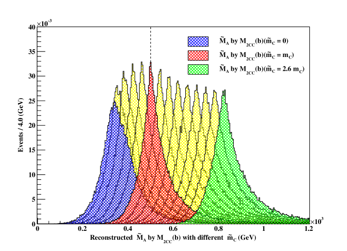
Figure 11: The same as Fig. 10, this time reconstructing the mass, $\tilde{M}_{A}$, of the relative particle in subsystem $(b)$ for several values of $\tilde{m}_{C}$, using invisible momenta from $M_{2CC}(b)$. The red shaded distribution corresponds to the true value, $\tilde{m}_{C}=m_{C}$, and is the same as the red histogram in the right panel of Fig. 9. The vertical black dashed line marks the true mass, $m_{A}=500$ GeV, in our example.

The function, (50), can be experimentally derived as shown in Fig. 11 — one varies the test mass, $\tilde{m}_{C}$, and forms a series of $\tilde{M}_{A}$ distributions. The location of the peak of each distribution represents the value of $\tilde{m}_{A}$ for the given hypothesized value of $\tilde{m}_{C}$. The red shaded histogram in Fig. 11 corresponds to the true value of $\tilde{m}_{C}=m_{C}$ and again peaks at the correct value of the mass, $m_{A}$, of the relative particle:

$$m_{A}=\tilde{M}_{A}^{peak}(b)(m_{C}).$$ (51)

Finally, one may also consider the subsystem $(a)$ and study the distributions of the reconstructed relative mass, $\tilde{M}_{C}$, shown in the middle panel of Fig. 9. This establishes the relation

$$\tilde{m}_{C}(\tilde{m}_{B})=\tilde{M}_{C}^{peak}(a)(\tilde{m}_{B}).$$ (52)

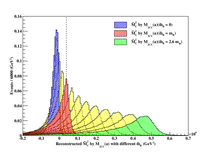
Figure 12: The same as Fig. 10, this time reconstructing the mass squared, $\tilde{M}_{C}^{2}$, of the relative particle in subsystem $(a)$ for several values of $\tilde{m}_{B}$, using invisible momenta from $M_{2CC}(a)$. The red shaded distribution corresponds to the true value, $\tilde{m}_{B}=m_{B}$, and is the same as the red histogram in the middle panel of Fig. 9. The vertical black dashed line marks the value of the true mass squared, $m_{C}^{2}=40,000\ {\rm GeV}^{2}$, in our example.

The procedure is illustrated in Fig. 12, where we have used $M_{2CC}(a)$ to fix the momenta of the invisible particles before computing $\tilde{M}_{C}^{2}$. A peculiar feature of Fig. 12 is that for low enough values of the test mass, $\tilde{m}_{B}$, the peak of the distribution is found at negative values of $\tilde{M}_{C}^{2}$, which is why we do not take a square root and instead use the mass squared in the plot. Nevertheless, the important feature of Fig. 12 is that, just like in Figs. 10 and 11, for the correct choice of the test mass, $\tilde{m}_{B}=m_{B}$ (see red histogram), the peak reveals the true value, $m_{C}$, of the relative particle (in this case $C_{i}$).

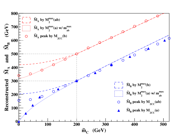
Figure 13: A summary of the different mass correlation methods discussed in the text: (53) is represented by a blue dashed line, (54) is given by a red dashed line, (57) is shown by the red open circles, (58) is denoted by the blue open circles, while (59) is marked by the blue triangles. The red dotted line represents the relationship between $\tilde{m}_{A}$ and $\tilde{m}_{C}$ which is obtained by eliminating $\tilde{m}_{B}$ from (55) and (56), while the blue dotted line shows the orthogonal relationship among $\tilde{m}_{B}$ and $\tilde{m}_{C}$ resulting from eliminating $\tilde{m}_{A}$ from (55) and (56).

Before concluding, in Fig. 13 we summarize the different mass determination methods discussed in this section. The existing method relies on measuring $M_{T2}$ kinematic endpoints in the three subsystems of Fig. 2, establishing the three relationships (44), (48), and (49). In Sec. 4.1, we proposed to measure the sharper $M_{2CC}$ kinematic endpoints instead, resulting in three analogous relations

$$\tilde{m}_{B}(\tilde{m}_{C}) = M_{2}^{max}(b)(\tilde{m}_{C}),$$ (53)

$$\tilde{m}_{A}(\tilde{m}_{C}) = M_{2}^{max}(ab)(\tilde{m}_{C}),$$ (54)

$$\tilde{m}_{A}(\tilde{m}_{B}) = M_{2}^{max}(a)(\tilde{m}_{B}).$$ (55)

These can be supplemented with the classic measurement of the kinematic endpoint of the invariant mass, $M_{ab}$, of the two visible particles, $a_{i}$ and $b_{i}$, in each decay chain

$$M_{ab}^{max}=\sqrt{\frac{(\tilde{m}_{A}^{2}-\tilde{m}_{B}^{2})(\tilde{m}_{B}^{2}-\tilde{m}_{C}^{2})}{\tilde{m}_{B}^{2}}},$$ (56)

which provides a constraint among all three masses $\tilde{m}_{A}$, $\tilde{m}_{B}$, and $\tilde{m}_{C}$. The four measurements (53-56) are already sufficient to determine the three unknowns $\tilde{m}_{A}$, $\tilde{m}_{B}$, and $\tilde{m}_{C}$ Burns:2008va . The new measurements proposed in Sec. 4.2 are the peak determinations

$$\tilde{m}_{A}(\tilde{m}_{C}) = \tilde{M}_{A}^{peak}(b)(\tilde{m}_{C}),$$ (57)

$$\tilde{m}_{B}(\tilde{m}_{C}) = \tilde{M}_{B}^{peak}(ab)(\tilde{m}_{C}),$$ (58)

$$\tilde{m}_{C}(\tilde{m}_{B}) = \tilde{M}_{C}^{peak}(a)(\tilde{m}_{B}).$$ (59)

The seven relations (53-59) are pictorially illustrated in Fig. 13. In order to display all seven relations on the same plot, we first plot (53-54) and (57-59) directly, then from the remaining two relations (55) and (56) we either eliminate $\tilde{m}_{B}$ to obtain $\tilde{m}_{A}$ as a function of $\tilde{m}_{C}$ (red dotted line), or eliminate $\tilde{m}_{A}$ to obtain $\tilde{m}_{B}$ as a function of $\tilde{m}_{C}$ (blue dotted line). All seven correlations (53-59) agree for the correct values for $m_{A}$, $m_{B}$ and $m_{C}$, marked with the black dotted lines in Fig. 13. What is more interesting is that they disagree for the wrong values of the test input mass, $\tilde{m}_{C}$. This is particularly noticeable in the region $\tilde{m}_{C}<m_{C}$. Fig. 13 suggests that by combining the results from all the different methods (53-59) one can determine the true value of $m_{C}$ as the location of the crossing point of the different curves shown in the figure. Our method is complementary to other methods in the literature for determining the absolute value of $m_{C}$ Cho:2007qv ; Gripaios:2007is ; Barr:2007hy ; Cho:2007dh ; Barr:2009jv ; Matchev:2009ad ; Matchev:2009fh ; Alwall:2009sv ; Konar:2009wn ; Cohen:2010wv ; Cheng:2011ya ; Serna:2008zk .

5 Using $M_{2}$ variables for topology disambiguation

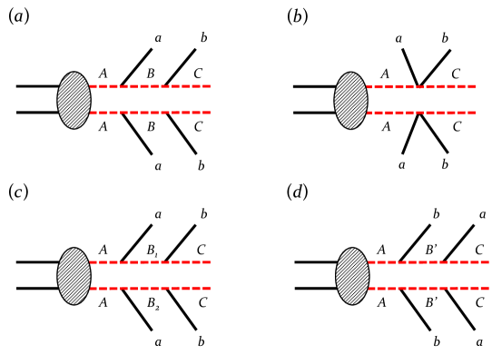
Figure 14: The four benchmark decay topologies studied in Sec. 5.

Up to this point, we have been studying events under the correct assumption about the event topology. However, in a real experiment, there is no prior indication as to what the correct event topology is for any given observed final state, and one should consider (and test for) all possible alternatives. This is exactly what we set out to do in this section. Given our observed final state of two visible $a$ particles, two visible $b$ particles and missing transverse momentum, a number of event topologies are possible; four of which are shown in Fig. 14. Fig. 14(a) shows our nominal scenario, (43), considered so far, in which there is an on-shell $B_{i}$ resonance in each chain and furthermore, the two $B$ resonances are the same: $B_{1}=B_{2}\equiv B$. Fig. 14(b) represents the off-shell scenario in which the intermediate $B$ resonance is very heavy and the decays are three-body. Fig. 14(c) is the same as Fig. 14(a), but with a slight modification — now the two intermediate resonances, $B_{i}$, are different: $B_{1}\neq B_{2}$. Finally, Fig. 14(d) is the analogue of Fig. 14(a) in which the visible particles, $a$ and $b$, are switched, i.e., the decay to $b$ takes place first, followed by the decay to $a$.

In this section, we shall design several tests which discriminate among the alternative possibilities depicted in Fig. 14. The tests make crucial use of the constrained $M_{2}$ variables introduced in Sec. 2.

5.1 Endpoint test

We first design a test to distinguish among the three event topologies shown in Fig. 14(a), Fig. 14(b), and Fig. 14(c). (This test will not be able to discriminate among Fig. 14(a) and Fig. 14(d).) The basic idea is very simple. Recall that the $M_{2XC}(ab)$ and $M_{2CC}(ab)$ variables from Sec. 2 were defined under the assumption of a common relative particle. I.e.,

• there is an intermediate $B_{i}$ resonance in each decay chain, and

• the two $B_{i}$ particles are the same, so that $m_{B_{1}}=m_{B_{2}}$.

If either of these two assumptions is incorrect, the definition of $M_{2XC}(ab)$ and $M_{2CC}(ab)$ loses its physical meaning, and as a result something will go wrong. Therefore, by testing for the consistency of $M_{2XC}(ab)$ and $M_{2CC}(ab)$ with another, topology-independent, variable like $M_{2XX}(ab)$, we can verify the above two assumptions. Note that relaxing the first assumption leads to the event topology of Fig. 14(b), while dropping the second assumption leads to the event topology of Fig. 14(c).

How can one test for the consistency of $M_{2XC}(ab)$ and $M_{2CC}(ab)$? Recall that the basic property of all $M_{2}$ variables is that they provide a lower bound on the mass of the corresponding parent, and their upper kinematic endpoints saturate that bound, revealing the mass of the parent (as a function of the test daughter mass). Now consider the relevant variables (14) for subsystem $(ab)$. They bound the mass of the same parent $A$, the only difference is that they have various assumptions about the event topology built in. Therefore, if all those assumptions are correct, the kinematic endpoints of all the variables should agree as well:

$$M_{T2}^{max}=M_{2XX}^{max}=M_{2CX}^{max}=M_{2XC}^{max}=M_{2CC}^{max}.$$ (60)

Conversely, if some of the assumptions are not satisfied, (60) will be violated — there will be a certain number of events in which the values of $M_{2XC}(ab)$ and $M_{2CC}(ab)$ will violate the upper kinematic endpoint $M_{2XX}^{max}$ of the topology-independent variable $M_{2XX}(ab)$.

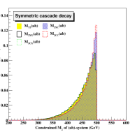
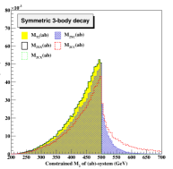
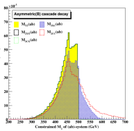
Figure 15: The same as the upper left panel of Fig. 8, but using events from three different scenarios. The left panel shows the nominal event topology from Fig. 14(a) with $(m_{A},\;m_{B},\;m_{C})=(500,\;300,\;200)$ GeV. The middle panel corresponds to the off-shell case of Fig. 14(b) with $(m_{A},\;m_{C})=(500,\;200)$ GeV. The right panel represents the asymmetric event topology from Fig. 14(c) with $(m_{A},\;m_{B_{2}},\;m_{B_{1}},\;m_{C})=(500,\;400,\;300,\;200)$ GeV. The test mass was always chosen to be $\tilde{m}_{C}=200$ GeV.

The test is performed in Fig. 15, where we compare the distributions of the five variables in the $(ab)$ subsystem, as in the upper left panel of Fig. 8. In the left panel of Fig. 15, we first consider the case of our nominal event topology from Fig. 14(a) with the mass spectrum from (43). As already observed in Fig. 8, the distributions may have slightly different shapes, but their endpoints are exactly the same. Therefore, this case passes the endpoint test, (60), as expected.

We next consider the off-shell case of Fig. 14(b) with $(m_{A},\;m_{C})=(500,\;200)$ GeV and plot the results in the middle panel of Fig. 15. In accordance with the equivalence theorem from Sec. 3.1, the distributions of $M_{T2}$, $M_{2XX}$, and $M_{2CX}$ are identical, and their common endpoint provides a reference value, $M_{2XX}^{max}$, to be compared against the endpoints of $M_{2XC}$ and $M_{2CC}$. The plot clearly shows that the distributions of $M_{2XC}$ and $M_{2CC}$ develop long tails beyond $M_{2XX}^{max}$, thus violating (60) and failing the endpoint test. The violation is more severe in the case of $M_{2CC}$ (the red histograms in Fig. 15), where a larger number of events have migrated beyond the anticipated endpoint $M_{2XX}^{max}$. The reason for this violation is easy to understand — in the off-shell case of Fig. 14(b) there are no intermediate resonances, $B_{1}$ and $B_{2}$. Thus when we enforce the relative constraint, $M_{B_{1}}=M_{B_{2}}$, in constructing the $M_{2XC}$ and $M_{2CC}$ variables, we unnecessarily restrict the range of allowed values of the invisible momenta during the minimization, and thus arrive at an unphysical global minimum. Based on the results from the middle panel of Fig. 15, we can therefore safely rule out the on-shell event topology of Fig. 14(a) as being the source of these events.

The right panel in Fig. 15 shows the case of the asymmetric event topology from Fig. 14(c) with $(m_{A},\;m_{B_{2}},\;m_{B_{1}},\;m_{C})=(500,\;400,\;300,\;200)$ GeV. This time, the intermediate resonances, $B_{1}$ and $B_{2}$, are present, but their masses are not equal: $m_{B_{1}}=300$ GeV, while $m_{B_{2}}=400$ GeV. Thus applying the relative constraint, $M_{B_{1}}=M_{B_{2}}$, during the minimization for $M_{2XC}$ and $M_{2CC}$ once again leads to an unphysical situation. As a result, the $M_{2XC}$ and $M_{2CC}$ distributions again develop tails beyond $M_{2XX}^{max}$, failing the test (60) and ruling out the on-shell event topology of Fig. 14(a) as being the source of these events.

Note that in the last two cases, when the endpoint test failed, it simply told us which event topology is wrong, but it did not specify the correct answer. For this, we must develop further tests as in the next two subsections. However, notice the distinctive shape of the distributions in the right panel of Fig. 15 in comparison with the middle panel. One might hope to use this shape difference to further discriminate among the event topologies of Fig. 14(b) and Fig. 14(c). However, such detailed shape analysis is beyond the scope of this paper.

Note that the ability to discriminate among two alternative event topologies suggests an interesting application of the constrained $M_{2}$ variables in discriminating the signal from irreducible backgrounds newpaper . The SM backgrounds have known event topologies, for which the corresponding on-shell constraints can be readily applied; the resulting distributions will still have the same endpoint. With a suitably chosen cut above this expected SM endpoint, one would be able to remove most, if not all, background events. On the other hand, the signal event topology is generally different, and the signal events will migrate to higher values of $M_{2}$ once the kinematic constraints are imposed, leading to a higher signal efficiency when using $M_{2}$ in place of $M_{T2}$.

5.2 Dalitz plot test

In this subsection, we develop a Dalitz plot test which enables us to discriminate the event topology in Fig. 14$(a)$ from those in 14$(b)$ and 14$(d)$. The idea is to use the invisible momenta obtained in the $M_{2}$ minimization to form invariant mass combinations involving the final state invisible particles, $C_{i}$.

To see how the method works, let us assume that the signal comes from the event topology of Fig. 14$(a)$. First consider the ideal case when we have exact knowledge of the four momenta of the invisible particles, $C_{i}$. Since there are three particles in the final state of each decay chain, $a_{i}$, $b_{i}$, and $C_{i}$, and we know their 4-momenta, we can form three invariant mass combinations, $M_{ab}$, $M_{bC}$, and $M_{aC}$. Since particles $b_{i}$ and $C_{i}$ originate from the same mother particle, $B_{i}$, $M_{bC}$ simply equals the mass, $m_{B}$, of that mother particle, regardless of the value of $M_{ab}$. Therefore, the Dalitz plot in the $(M_{bC}^{2},M_{ab}^{2})$ plane is characterized by a single vertical line:

$$M_{bC}^{2}=m_{B}^{2}\hskip 28.45274pt\hbox{for any }M_{ab}^{2}\in[0,(M_{ab}^{\max})^{2}],$$ (61)

with $M_{ab}^{max}$ given by (56). On the other hand, $M_{aC}^{2}$ takes values within a given range consistent with the sum rule

$$M_{aC}^{2}=m_{A}^{2}-m_{B}^{2}+m_{C}^{2}-M_{ab}^{2}\hskip 28.45274pt\hbox{for any }M_{ab}^{2}\in[0,(M_{ab}^{\max})^{2}],$$ (62)

which is nothing but a straight line with a negative slope in the plane of $(M_{aC}^{2},M_{ab}^{2})$. The predictions (61) and (62) in this idealized case are illustrated in the upper left panel of Fig. 16, where the vertical line corresponds to (61), and the slanted line corresponds to (62).

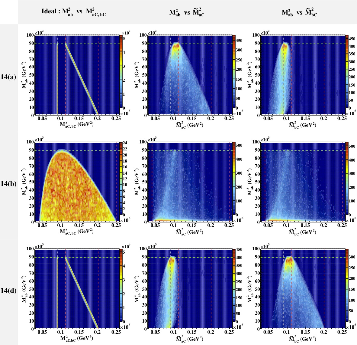
Figure 16: Dalitz plots for the event topologies of Fig. 14$(a)$ (top row), Fig. 14$(b)$ (middle row), and Fig. 14$(d)$ (bottom row). Using the invisible particle momenta obtained from $M_{2CC}(ab)$, we show scatter plots of $\tilde{M}_{aC}^{2}$ versus $M_{ab}^{2}$ (middle column) and $\tilde{M}_{bC}^{2}$ versus $M_{ab}^{2}$ (right column). The left column shows the corresponding results in the ideal case when we use the true momenta of the invisible particles in the event. The mass spectrum is fixed as in (43).

We are now ready to consider the more realistic case in which we do not have exact knowledge of the individual momenta of the invisible particles, $C_{i}$, but instead obtain them from the $M_{2CC}$ ansatz. The corresponding results are shown in the remaining two plots in the top row of Fig. 16 — the middle panel shows a scatter plot in the $(M_{aC}^{2},M_{ab}^{2})$ plane, while the right panel shows a scatter plot in the $(M_{bC}^{2},M_{ab}^{2})$ plane. Since the invisible momenta are only approximated, the correlations are not exactly linear, but nevertheless they tend to follow the general trends given by (61) and (62).

Let us now move on to the event topology of Fig. 14(b). This case is illustrated in the middle row of Fig. 16. Since the intermediate $B_{i}$ resonance is absent, the visible particles, $a_{i}$ and $b_{i}$, arise from the same vertex and are on equal footing. Thus, we expect the associated Dalitz plots in the $(M_{aC}^{2},M_{ab}^{2})$, and $(M_{bC}^{2},M_{ab}^{2})$ planes to be very similar, and indeed this is what we observe by comparing the middle and right panels of the middle row. We therefore conclude that the similarity between the two Dalitz plots is an indication of an off-shell scenario as in Fig. 14(b).

Finally, the bottom row in Fig. 16 represents the case of the event topology from Fig. 14(d), which again has a pair of identical intermediate resonances, $B_{i}$, only now the visible particles, $a_{i}$ and $b_{i}$, are emitted in the opposite order — $b_{i}$ comes first and $a_{i}$ comes second. Comparing this to the decay topology of Fig. 14(a), we see that the only difference is that the roles of the visible particles, $a_{i}$ and $b_{i}$, are reversed. Therefore our previous analysis leading up to eqs. (61) and (62) still applies, only now the two trends are interchanged — the correlation in the $(M_{aC}^{2},M_{ab}^{2})$ plane is expected to be a vertical straight line, while the correlation in the $(M_{bC}^{2},M_{ab}^{2})$ plane is expected to be a slanted straight line. This ideal case with perfect knowledge of the invisible momenta is shown in the left bottom panel of Fig. 16. The more realistic case, in which the invisible momenta are taken from the $M_{2CC}(ab)$ minimization, is presented in the middle and right bottom panels of Fig. 16. As expected, the behavior is exactly the opposite of what we observed in the corresponding plots in the upper row of Fig. 16. Our conclusion, therefore, is that whenever the two scatter plots are different, the visible particle in the scatter plot with the vertical correlation is the one which is emitted second, while the visible particle in the slanted scatter plot is the one which is emitted first.

5.3 Resonance scatter plot test

Finally, we describe a test aimed at detecting and identifying any intermediate resonances, $B_{i}$. In particular, we shall revisit the event topologies from Figs. 14(a), 14(b), and 14(c) and attempt to answer the questions:

• Is there an intermediate $B_{i}$ resonance in each decay chain?

• If so, are the two $B_{i}$ particles the same or not?

Once again, the idea is to use the invisible momenta found by one of the $M_{2}$-type minimizations and then reconstruct the masses of the hypothesized $B_{i}$ resonances. As already discussed in Sec. 3, the novel advantage of the $M_{2}$-type variables (e.g., over transverse variables like $M_{T2}$) is that they supply the full 3-momenta of the invisible particles, including the longitudinal components. Thus, it becomes possible to carry out the direct reconstruction of any heavy particles along the decay chain. In our case, to form the mass of particle $B_{i}$, we simply use the measured 4-momentum of $b_{i}$ and the momentum of $C_{i}$ obtained in the minimization of $M_{2CX}(ab)$. In order to avoid the two-fold ambiguity discussed in Sec. 3.2, we use only “balanced” events, for which the invisible momentum configuration is unique.

Since each event contains two decay chains, we will obtain two reconstructed values per event, $\tilde{M}_{B_{1}}$ and $\tilde{M}_{B_{2}}$, which we order as usual as

$$\tilde{M}_{B}^{>} = \max\left\{\tilde{M}_{B_{1}},\tilde{M}_{B_{2}}\right\},$$ (63)

$$\tilde{M}_{B}^{<} = \min\left\{\tilde{M}_{B_{1}},\tilde{M}_{B_{2}}\right\}.$$ (64)

We then investigate the resonance structure of the corresponding scatter plot in the $(\tilde{M}_{B}^{>},\tilde{M}_{B}^{<})$ plane, as shown in Fig. 17.

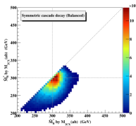
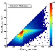
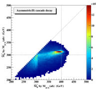
Figure 17: Scatter plots of the reconstructed masses of the two intermediate resonances, $\tilde{M}_{B_{1}}$ and $\tilde{M}_{B_{2}}$, for the three scenarios from Fig. 15, with invisible momenta taken from the $M_{2CX}(ab)$ minimization. The larger of the two reconstructed masses, $\tilde{M}_{B}^{>}$, is plotted on the $x$-axis, while the smaller of the two reconstructed masses, $\tilde{M}_{B}^{<}$, is plotted on the $y$-axis. The vertical and horizontal black dashed lines denote the true masses of the associated relative particles.

The left panel in Fig. 17 represents the case of the event topology from Fig. 14(a), which has two identical intermediate resonances, $B_{1}$ and $B_{2}$. Correspondingly, the scatter plot exhibits a distinct clustering of events near the diagonal line ($\tilde{M}_{B}^{>}=\tilde{M}_{B}^{<}$), indicating the presence of such identical resonances. Furthermore, we can also roughly read the mass scale as $M_{B_{i}}\sim 300$ GeV (compare with the true values marked with the black dashed lines). Now contrast this situation with the case of the event topology from Fig. 14(c), which is shown in the rightmost panel of Fig. 17. Again, we find a narrow clustering of points, indicating the presence of intermediate $B_{i}$ resonances. Now, however, the cluster lies significantly far from the diagonal line, implying that the intermediate resonances are different. The location of the cluster is also consistent with the input mass spectrum ($m_{B_{1}}=300$ GeV, $m_{B_{2}}=400$ GeV, as indicated with the black dashed lines).

The third example, shown in the middle panel of Fig. 17, is the event topology from Fig. 14(b). The two decay chains are the same, so we expect most of the events to end up near the diagonal line $\tilde{M}_{B}^{>}=\tilde{M}_{B}^{<}$. However, since there are no intermediate resonances, we do not expect a significant clustering in any particular location and instead would expect a broader distribution that in the previous two resonant cases. These expectations are confirmed in Fig. 17 — the middle panel exhibits a large population near the diagonal line whose structure differs from that in the left panel, allowing us to distinguish the topology of Fig. 14(b) from the topology of Fig. 14(a). Again, we defer a more detailed shape analysis to future work.

6 Conclusions and outlook

The main goal of this paper is to advocate a wider use of the 3+1-dimensional $M_{2}$-type variables, which so far have been used only sporadically  Ross:2007rm ; Barr:2008ba ; Barr:2011xt ; Mahbubani:2012kx . In contrast, transverse mass variables like $M_{T}$, $M_{T2}$, $M_{CT}$, etc. have found widespread application in both precision measurements Chatrchyan:2013boa ; ATLAS:2012poa and in searches for new physics Chatrchyan:2012jx ; TheATLAScollaboration:2013xha . There are two main advantages of the 3+1-dimensional formulation in terms of $M_{2}$:

1. It is very easy to impose various additional assumptions about the underlying event topology Mahbubani:2012kx . In this paper we illustrated this feature with the addition of on-shell constraints for the relative particles, which led us to two new variables, $M_{2XC}$ and $M_{2CC}$. The benefits from $M_{2XC}$ and $M_{2CC}$ are twofold — first, the solution for the longitudinal invisible momenta is unique, as discussed in Sec. 3.3, and second, their distributions exhibit much sharper endpoints, as demonstrated in Sec. 4.1.

2. The minimization procedure required to calculate the value of $M_{2}$ fixes all components of the invisible particle momenta, including the longitudinal components. This gives an event with fully determined kinematics, opening the door for a number of precision reconstruction studies. As an illustration, in Sec. 4.2, we reconstructed the mass of the relative particle and showed that the peak of the resulting distribution is nicely correlated with the true mass of the relative particle. This provides a new technique for mass measurements in missing energy events, which is complementary to the existing methods based on measuring kinematic endpoints.

It is interesting to note that even for a process as simple as the one studied here (see Fig. 1), we were able to define a relatively large number of $M_{2}$-type variables, summarized in Table 2. While the casual reader might feel intimidated by this proliferation of kinematic mass variables, we emphasize that there is a great benefit in having such a large arsenal of kinematic variables at one’s disposal. The main reason why there are so many variables is that each involves different levels of assumptions. Thus, by testing for consistency of the results obtained with two different variables, we are essentially checking the validity of the assumptions that are present in one of the variables but not the other.

Following this idea, we developed several tests for distinguishing among the alternative event topologies of Fig. 14, which lead to the same final state:

• Endpoint test. In Sec. 5.1, we proposed a test which compares the endpoints of the distributions of $M_{2}$ variables with and without relative constraints. If the constraints are satisfied in the event sample, the kinematic endpoints would match (even though the shapes of the distributions are generally different). Conversely, if the mass constraints are not satisfied, the endpoints will be different, which is an indication that our hypothesis regarding the event topology is wrong. We have checked that this test is applicable even when one does not have precise knowledge of the daughter mass.

• Dalitz plot test. In Sec. 5.2, we used the fact that the computation of the $M_{2}$ variables supplies values for the 4-momenta of the invisible particles and proposed to build Dalitz-type plots of invariant mass combinations which include the invisible particles themselves (see Fig. 16). We showed that the distinctive shape of the Dalitz scatter plots can be used to ascertain the presence of intermediate resonances and to resolve the combinatorial ambiguity related to the ordering of the visible final state particles along the decay chain.

• Resonance scatter plot test. The invisible momenta supplied by $M_{2}$ found another application in Sec. 5.3, where we were able to test for the symmetry of the events, i.e., whether the two decay chains are the same or not (see Fig. 17).

These are just a few of the many potential applications of the $M_{2}$ variables — for example, one could imagine spin measurements along the lines of Cho:2008tj ; Cheng:2010yy ; Guadagnoli:2013xia , using the invisible particle momenta supplied by the $M_{2}$ minimizations. It is also possible to further extend the set of variables from Table 2 to more complicated event topologies — e.g., decay chains with more than one relative particle, decay chains with relatives of known mass, etc. One technical problem which will need to be addressed in the near future is the lack of a public code for the calculation of the on-shell constrained $M_{2}$ variables. The availability of such code would certainly encourage more experimentalists to make use of these variables whose benefits seem undeniable.

Appendix A Proof that $M_{T2}=M_{2CX}$ with the method of Lagrange multipliers

In this appendix, we show the equivalence between $M_{T2}$ and $M_{2CX}$ using the method of Lagrange multipliers. For concreteness, the formal proof is presented for the $(ab)$ subsystem, but the same argument can be applied to the other subsystems, $(a)$ and $(b)$, as well.

In order to calculate $M_{2CX}^{2}(ab)$, we must perform the minimization of the function

$$\max\left[M_{A_{1}}^{2}(\vec{q}_{1T},\;\Delta\eta_{1};\;\tilde{m}),\;M_{A_{2}}^{2}(\vec{q}_{2T},\;\Delta\eta_{2};\;\tilde{m})\right],$$ (65)

subject to the two constraints

$$M_{A_{1}}^{2}(\vec{q}_{1T},\;\Delta\eta_{1};\;\tilde{m}) = M_{A_{2}}^{2}(\vec{q}_{2T},\;\Delta\eta_{2};\;\tilde{m}),$$ (66)

$$\vec{q}_{1T}+\vec{q}_{2T} = {\;/\!\!\!\!\vec{P}_{T}}.$$ (67)

Here we have already assumed that the hypothesized masses of the daughter particles, $C_{i}$, are the same, so that there is a single input test mass, $\tilde{m}$. We have also expressed the parent masses, $M_{A_{i}}$, as functions of $\Delta\eta_{i}$ instead of $q_{iz}$, as in (20).

We can use the method of Lagrange multipliers to reformulate the problem as the unconstrained minimization of a new target function

$$f(\vec{q}_{1T},\vec{q}_{2T},\Delta\eta_{1},\Delta\eta_{2},\vec{\lambda}_{T},\lambda_{\eta};\tilde{m})$$ (68)

$$=\frac{1}{2}\left\{E_{v_{1}T}E_{q_{1}T}\cosh\Delta\eta_{1}-\vec{p}_{v_{1}T}\cdot\vec{q}_{1T}+E_{v_{2}T}E_{q_{2}T}\cosh\Delta\eta_{2}-\vec{p}_{v_{2}T}\cdot\vec{q}_{2T}\right\}$$

$$+\lambda_{\eta}\left\{E_{v_{1}T}E_{q_{1}T}\cosh\Delta\eta_{1}-\vec{p}_{v_{1}T}\cdot\vec{q}_{1T}-E_{v_{2}T}E_{q_{2}T}\cosh\Delta\eta_{2}+\vec{p}_{v_{2}T}\cdot\vec{q}_{2T}\right\}$$

$$+\vec{\lambda}_{T}\cdot(\vec{q}_{1T}+\vec{q}_{2T}-{\;/\!\!\!\!\vec{P}_{T}}),$$

which needs to be minimized over all of its arguments: $\vec{q}_{1T}$, $\vec{q}_{2T}$, $\Delta\eta_{1}$, $\Delta\eta_{2}$, $\vec{\lambda}_{T}$, and $\lambda_{\eta}$. The constraint (66) is implemented through the Lagrange multiplier $\lambda_{\eta}$, while the constraint (67) is incorporated through the Lagrange multiplier $\vec{\lambda}_{T}$. In view of the constraint (66) in the first term we have replaced (65) with the average of $M_{A_{1}}^{2}$ and $M_{A_{2}}^{2}$.

The extremum conditions for $\vec{q}_{iT}$ and $\Delta\eta_{i}$ read:

$$\vec{\triangledown}_{q_{1T}}f = \left(\frac{1}{2}+\lambda_{\eta}\right)\left(\frac{E_{v_{1}T}}{E_{q_{1}T}}\cosh\Delta\eta_{1}\vec{q}_{1T}-\vec{p}_{v_{1}T}\right)+\vec{\lambda}_{T}=0,$$ (69)

$$\vec{\triangledown}_{q_{2T}}f = \left(\frac{1}{2}-\lambda_{\eta}\right)\left(\frac{E_{v_{2}T}}{E_{q_{2}T}}\cosh\Delta\eta_{2}\vec{q}_{2T}-\vec{p}_{v_{2}T}\right)+\vec{\lambda}_{T}=0,$$ (70)

$$\frac{\partial f}{\partial\Delta\eta_{1}} = \left(\frac{1}{2}+\lambda_{\eta}\right)E_{v_{1}T}E_{q_{1}T}\sinh\Delta\eta_{1}=0,$$ (71)

$$\frac{\partial f}{\partial\Delta\eta_{2}} = \left(\frac{1}{2}-\lambda_{\eta}\right)E_{v_{2}T}E_{q_{2}T}\sinh\Delta\eta_{2}=0.$$ (72)

There are two cases which can be considered separately: i) $\lambda_{\eta}=1/2$ (or $\lambda_{\eta}=-1/2$), and ii) $\lambda_{\eta}\neq\pm 1/2$.

i) $\lambda_{\eta}=1/2$:

Since $\lambda_{\eta}=1/2$, (72) is automatically solved, so $\Delta\eta_{2}$ remains arbitrary. Then (70) implies $\vec{\lambda}_{T}=0$, and from (71) it follows that $\Delta\eta_{1}=0$. Finally, (69) leads to $\vec{q}_{1T}=\frac{E_{q_{1}T}}{E_{v_{1}T}}\vec{p}_{v_{1}T}$. Substituting these results into (68), we get

$$f=E_{v_{1}T}E_{q_{1}T}-\vec{p}_{v_{1}T}\cdot\vec{q}_{1T}=M_{TA_{1}}^{2}(ab),$$ (73)

which is nothing but the transverse mass of $A_{1}$ as given in (16). This implies that minimizing $f$ is equivalent to minimizing the transverse mass of $A_{1}$.

The same logic can be applied to the case $\lambda_{\eta}=-1/2$, where one finds that the problem reduces to the minimization of the transverse mass of $A_{2}$. Thus we conclude that these two cases with $|\lambda|=\frac{1}{2}$ simply correspond to the unbalanced configuration of the $M_{T2}(ab)$ variable.

ii) $\lambda_{\eta}\neq\pm 1/2$:

Since $\lambda_{\eta}\neq\pm 1/2$, the only way to satisfy Eqs. (71) and (72) is to have $\Delta\eta_{i}=0$. This reduces the function (68) to

$$f = \frac{1}{2}(M_{TA_{1}}^{2}(ab)+M_{TA_{2}}^{2}(ab))+\lambda_{\eta}(M_{TA_{1}}^{2}(ab)-M_{TA_{2}}^{2}(ab))$$ (74)

$$+ \vec{\lambda}_{T}\cdot(\vec{q}_{1T}+\vec{q}_{2T}-{\;/\!\!\!\!\vec{P}_{T}}),$$

which is nothing but the Lagrange function associated with the balanced solution of the corresponding $M_{T2}$ variable.

From i) and ii) we see that $M_{2CX}(ab)$ includes both the balanced and the unbalanced configurations of $M_{T2}(ab)$, thus it follows that $M_{2CX}(ab)=M_{T2}(ab)$.

References

- (1) A. J. Barr and C. G. Lester, “A Review of the Mass Measurement Techniques proposed for the Large Hadron Collider,” J. Phys. G 37, 123001 (2010) [arXiv:1004.2732 [hep-ph]].
- (2) L. -T. Wang and I. Yavin, “A Review of Spin Determination at the LHC,” Int. J. Mod. Phys. A 23, 4647 (2008) [arXiv:0802.2726 [hep-ph]].
- (3) I. Hinchliffe, F. E. Paige, M. D. Shapiro, J. Soderqvist and W. Yao, “Precision SUSY measurements at CERN LHC,” Phys. Rev. D 55, 5520 (1997) [hep-ph/9610544].
- (4) H. Bachacou, I. Hinchliffe and F. E. Paige, “Measurements of masses in SUGRA models at CERN LHC,” Phys. Rev. D 62, 015009 (2000) [hep-ph/9907518].
- (5) B. C. Allanach, C. G. Lester, M. A. Parker and B. R. Webber, “Measuring sparticle masses in nonuniversal string inspired models at the LHC,” JHEP 0009, 004 (2000) [hep-ph/0007009].
- (6) B. K. Gjelsten, D. J. Miller and P. Osland, “Measurement of SUSY masses via cascade decays for SPS 1a,” JHEP 0412, 003 (2004) [hep-ph/0410303].
- (7) B. K. Gjelsten, D. J. Miller and P. Osland, “Measurement of the gluino mass via cascade decays for SPS 1a,” JHEP 0506, 015 (2005) [hep-ph/0501033].
- (8) K. T. Matchev, F. Moortgat, L. Pape and M. Park, “Precise reconstruction of sparticle masses without ambiguities,” JHEP 0908, 104 (2009) [arXiv:0906.2417 [hep-ph]].
- (9) D. R. Tovey, “On measuring the masses of pair-produced semi-invisibly decaying particles at hadron colliders,” JHEP 0804, 034 (2008) [arXiv:0802.2879 [hep-ph]].
- (10) G. Polesello and D. R. Tovey, “Supersymmetric particle mass measurement with the boost-corrected contransverse mass,” JHEP 1003, 030 (2010) [arXiv:0910.0174 [hep-ph]].
- (11) K. T. Matchev and M. Park, “A General method for determining the masses of semi-invisibly decaying particles at hadron colliders,” Phys. Rev. Lett. 107, 061801 (2011) [arXiv:0910.1584 [hep-ph]].
- (12) M. M. Nojiri, D. Toya and T. Kobayashi, “Lepton energy asymmetry and precision SUSY study at hadron colliders,” Phys. Rev. D 62, 075009 (2000) [hep-ph/0001267].
- (13) H. -C. Cheng and J. Gu, “Measuring Invisible Particle Masses Using a Single Short Decay Chain,” JHEP 1110, 094 (2011) [arXiv:1109.3471 [hep-ph]].
- (14) K. Agashe, R. Franceschini and D. Kim, “A simple, yet subtle ’invariance’ of two-body decay kinematics,” Phys. Rev. D 88, 057701 (2013) [arXiv:1209.0772 [hep-ph]].
- (15) K. Agashe, R. Franceschini, D. Kim and K. Wardlow, “Using Energy Peaks to Count Dark Matter Particles in Decays,” Phys. Dark Univ. 2, 72 (2013) [arXiv:1212.5230 [hep-ph]].
- (16) K. Agashe, R. Franceschini and D. Kim, “Using Energy Peaks to Measure New Particle Masses,” arXiv:1309.4776 [hep-ph].
- (17) J. Smith, W. L. van Neerven and J. A. M. Vermaseren, “The Transverse Mass and Width of the Boson,” Phys. Rev. Lett. 50, 1738 (1983).
- (18) V. D. Barger, A. D. Martin and R. J. N. Phillips, “Perpendicular Mass From Decay,” Z. Phys. C 21, 99 (1983).
- (19) D. R. Tovey, “Measuring the SUSY mass scale at the LHC,” Phys. Lett. B 498, 1 (2001) [hep-ph/0006276].
- (20) P. Konar, K. Kong and K. T. Matchev, “ : A Global inclusive variable for determining the mass scale of new physics in events with missing energy at hadron colliders,” JHEP 0903, 085 (2009) [arXiv:0812.1042 [hep-ph]].
- (21) P. Konar, K. Kong, K. T. Matchev and M. Park, “RECO level and subsystem : Improved global inclusive variables for measuring the new physics mass scale in events at hadron colliders,” JHEP 1106, 041 (2011) [arXiv:1006.0653 [hep-ph]].
- (22) T. Robens, “ resurrected,” JHEP 1202, 051 (2012) [arXiv:1109.1018 [hep-ph]].
- (23) C. Rogan, “Kinematical variables towards new dynamics at the LHC,” arXiv:1006.2727 [hep-ph].
- (24) M. R. Buckley, J. D. Lykken, C. Rogan and M. Spiropulu, “Super-Razor and Searches for Sleptons and Charginos at the LHC,” arXiv:1310.4827 [hep-ph].
- (25) K. Kawagoe, M. M. Nojiri and G. Polesello, “A New SUSY mass reconstruction method at the CERN LHC,” Phys. Rev. D 71, 035008 (2005) [hep-ph/0410160].
- (26) M. M. Nojiri, G. Polesello and D. R. Tovey, “A Hybrid method for determining SUSY particle masses at the LHC with fully identified cascade decays,” JHEP 0805, 014 (2008) [arXiv:0712.2718 [hep-ph]].
- (27) H. -C. Cheng, D. Engelhardt, J. F. Gunion, Z. Han and B. McElrath, “Accurate Mass Determinations in Decay Chains with Missing Energy,” Phys. Rev. Lett. 100, 252001 (2008) [arXiv:0802.4290 [hep-ph]].
- (28) H. -C. Cheng, J. F. Gunion, Z. Han and B. McElrath, “Accurate Mass Determinations in Decay Chains with Missing Energy. II,” Phys. Rev. D 80, 035020 (2009) [arXiv:0905.1344 [hep-ph]].
- (29) H. -C. Cheng, Z. Han, I. -W. Kim and L. -T. Wang, “Missing Momentum Reconstruction and Spin Measurements at Hadron Colliders,” JHEP 1011, 122 (2010) [arXiv:1008.0405 [hep-ph]].
- (30) H. -C. Cheng, J. F. Gunion, Z. Han, G. Marandella and B. McElrath, “Mass determination in SUSY-like events with missing energy,” JHEP 0712, 076 (2007) [arXiv:0707.0030 [hep-ph]].
- (31) H. -C. Cheng and Z. Han, “Minimal Kinematic Constraints and m(T2),” JHEP 0812, 063 (2008) [arXiv:0810.5178 [hep-ph]].
- (32) C. G. Lester and D. J. Summers, “Measuring masses of semiinvisibly decaying particles pair produced at hadron colliders,” Phys. Lett. B 463, 99 (1999) [hep-ph/9906349].
- (33) A. Barr, C. Lester and P. Stephens, “m(T2): The Truth behind the glamour,” J. Phys. G 29, 2343 (2003) [hep-ph/0304226].
- (34) A. J. Barr, T. J. Khoo, P. Konar, K. Kong, C. G. Lester, K. T. Matchev and M. Park, “Guide to transverse projections and mass-constraining variables,” Phys. Rev. D 84, 095031 (2011) [arXiv:1105.2977 [hep-ph]].
- (35) W. S. Cho, K. Choi, Y. G. Kim and C. B. Park, “Gluino Stransverse Mass,” Phys. Rev. Lett. 100, 171801 (2008) [arXiv:0709.0288 [hep-ph]].
- (36) B. Gripaios, “Transverse observables and mass determination at hadron colliders,” JHEP 0802, 053 (2008) [arXiv:0709.2740 [hep-ph]].
- (37) A. J. Barr, B. Gripaios and C. G. Lester, “Weighing Wimps with Kinks at Colliders: Invisible Particle Mass Measurements from Endpoints,” JHEP 0802, 014 (2008) [arXiv:0711.4008 [hep-ph]].
- (38) W. S. Cho, K. Choi, Y. G. Kim and C. B. Park, “Measuring superparticle masses at hadron collider using the transverse mass kink,” JHEP 0802, 035 (2008) [arXiv:0711.4526 [hep-ph]].
- (39) M. Burns, K. Kong, K. T. Matchev and M. Park, “Using Subsystem for Complete Mass Determinations in Decay Chains with Missing Energy at Hadron Colliders,” JHEP 0903, 143 (2009) [arXiv:0810.5576 [hep-ph]].
- (40) C. G. Lester, “The stransverse mass, MT2, in special cases,” JHEP 1105, 076 (2011) [arXiv:1103.5682 [hep-ph]].
- (41) R. Mahbubani, K. T. Matchev and M. Park, “Re-interpreting the Oxbridge stransverse mass variable MT2 in general cases,” JHEP 1303, 134 (2013) [arXiv:1212.1720 [hep-ph]].
- (42) P. Konar, K. Kong, K. T. Matchev and M. Park, “Superpartner Mass Measurement Technique using 1D Orthogonal Decompositions of the Cambridge Transverse Mass Variable ,” Phys. Rev. Lett. 105, 051802 (2010) [arXiv:0910.3679 [hep-ph]].
- (43) A. J. Barr, B. Gripaios and C. G. Lester, “Transverse masses and kinematic constraints: from the boundary to the crease,” JHEP 0911, 096 (2009) [arXiv:0908.3779 [hep-ph]].
- (44) P. Konar, K. Kong, K. T. Matchev and M. Park, “Dark Matter Particle Spectroscopy at the LHC: Generalizing M(T2) to Asymmetric Event Topologies,” JHEP 1004, 086 (2010) [arXiv:0911.4126 [hep-ph]].
- (45) W. S. Cho, J. E. Kim and J. -H. Kim, “Amplification of endpoint structure for new particle mass measurement at the LHC,” Phys. Rev. D 81, 095010 (2010) [arXiv:0912.2354 [hep-ph]].
- (46) W. S. Cho, W. Klemm and M. M. Nojiri, “Mass measurement in boosted decay systems at hadron colliders,” Phys. Rev. D 84, 035018 (2011) [arXiv:1008.0391 [hep-ph]].
- (47) C. H. Lally and C. G. Lester, “Properties of MT2 in the massless limit,” arXiv:1211.1542 [hep-ph].
- (48) W. S. Cho, K. Choi, Y. G. Kim and C. B. Park, “M(T2)-assisted on-shell reconstruction of missing momenta and its application to spin measurement at the LHC,” Phys. Rev. D 79, 031701 (2009) [arXiv:0810.4853 [hep-ph]].
- (49) C. B. Park, “Reconstructing the heavy resonance at hadron colliders,” Phys. Rev. D 84, 096001 (2011) [arXiv:1106.6087 [hep-ph]].
- (50) G. G. Ross and M. Serna, “Mass determination of new states at hadron colliders,” Phys. Lett. B 665, 212 (2008) [arXiv:0712.0943 [hep-ph]].
- (51) A. J. Barr, G. G. Ross and M. Serna, “The Precision Determination of Invisible-Particle Masses at the LHC,” Phys. Rev. D 78, 056006 (2008) [arXiv:0806.3224 [hep-ph]].
- (52) K. Choi, S. Choi, J. S. Lee and C. B. Park, “Reconstructing the Higgs boson in dileptonic W decays at hadron collider,” Phys. Rev. D 80, 073010 (2009) [arXiv:0908.0079 [hep-ph]].
- (53) K. Choi, J. S. Lee and C. B. Park, “Measuring the Higgs boson mass with transverse mass variables,” Phys. Rev. D 82, 113017 (2010) [arXiv:1008.2690 [hep-ph]].
- (54) A. J. Barr, S. T. French, J. A. Frost and C. G. Lester, “Speedy Higgs boson discovery in decays to tau lepton pairs : ,” JHEP 1110, 080 (2011) [arXiv:1106.2322 [hep-ph]].
- (55) A. J. Barr, B. Gripaios and C. G. Lester, “Re-weighing the evidence for a Higgs boson in dileptonic W-boson decays,” Phys. Rev. Lett. 108, 041803 (2012) [Erratum-ibid. 108, 109902 (2012)] [arXiv:1108.3468 [hep-ph]].
- (56) A. J. Barr, B. Gripaios and C. GLester, “Finding Higgs bosons heavier than in dileptonic W-boson decays,” Phys. Lett. B 713, 495 (2012) [arXiv:1110.2452 [hep-ph]].
- (57) D. Guadagnoli and C. B. Park, “MT2-reconstructed invisible momenta as spin analyzers, and an application to top polarization,” arXiv:1308.2226 [hep-ph].
- (58) K. T. Matchev, F. Moortgat, L. Pape and M. Park, “Precision sparticle spectroscopy in the inclusive same-sign dilepton channel at LHC,” Phys. Rev. D 82, 077701 (2010) [arXiv:0909.4300 [hep-ph]].
- (59) J. Alwall, A. Freitas and O. Mattelaer, “Measuring Sparticles with the Matrix Element,” AIP Conf. Proc. 1200, 442 (2010) [arXiv:0910.2522 [hep-ph]].
- (60) T. Cohen, E. Kuflik and K. M. Zurek, “Extracting the Dark Matter Mass from Single Stage Cascade Decays at the LHC,” JHEP 1011, 008 (2010) [arXiv:1003.2204 [hep-ph]].
- (61) A. Rajaraman and F. Yu, “A New Method for Resolving Combinatorial Ambiguities at Hadron Colliders,” Phys. Lett. B 700, 126 (2011) [arXiv:1009.2751 [hep-ph]].
- (62) P. Baringer, K. Kong, M. McCaskey and D. Noonan, “Revisiting Combinatorial Ambiguities at Hadron Colliders with ,” JHEP 1110, 101 (2011) [arXiv:1109.1563 [hep-ph]].
- (63) K. Choi, D. Guadagnoli and C. B. Park, “Reducing combinatorial uncertainties: A new technique based on MT2 variables,” JHEP 1111, 117 (2011) [arXiv:1109.2201 [hep-ph]].
- (64) Y. Bai and H. -C. Cheng, “Identifying Dark Matter Event Topologies at the LHC,” JHEP 1106, 021 (2011) [arXiv:1012.1863 [hep-ph]].
- (65) W. S. Cho, D. Kim, K. T. Matchev and M. Park, “Cracking the dark matter code at the LHC,” arXiv:1206.1546 [hep-ph].
- (66) K. Agashe, D. Kim, M. Toharia and D. G. E. Walker, “Distinguishing Dark Matter Stabilization Symmetries Using Multiple Kinematic Edges and Cusps,” Phys. Rev. D 82, 015007 (2010) [arXiv:1003.0899 [hep-ph]].
- (67) K. Agashe, D. Kim, D. G. E. Walker and L. Zhu, “Using to Distinguish Dark Matter Stabilization Symmetries,” Phys. Rev. D 84, 055020 (2011) [arXiv:1012.4460 [hep-ph]].
- (68) G. F. Giudice, B. Gripaios and R. Mahbubani, “Counting dark matter particles in LHC events,” Phys. Rev. D 85, 075019 (2012) [arXiv:1108.1800 [hep-ph]].
- (69) S. Chatrchyan et al. [CMS Collaboration], “Measurement of masses in the system by kinematic endpoints in pp collisions at = 7 TeV,” Eur. Phys. J. C 73, 2494 (2013) [arXiv:1304.5783 [hep-ex]].
- (70) M. Serna, “A Short comparison between m(T2) and m(CT),” JHEP 0806, 004 (2008) [arXiv:0804.3344 [hep-ph]].
- (71) W. S. Cho, J. S. Gainer, D. Kim, K. Matchev, F. Moortgat, L. Pape, and M. Park, to appear.
- (72) [ATLAS Collaboration], “Top quark mass measurement in the channel using the variable at ATLAS,” ATLAS-CONF-2012-082.
- (73) S. Chatrchyan et al. [CMS Collaboration], “Search for supersymmetry in hadronic final states using in collisions at TeV,” JHEP 1210, 018 (2012) [arXiv:1207.1798 [hep-ex]].
- (74) The ATLAS collaboration, “Searches for direct scalar top pair production in final states with two leptons using the stransverse mass variable and a multivariate analysis technique in TeV pp collisions using 20.3 fb-1 of ATLAS data,” ATLAS-CONF-2013-065.