Manifold approach for a many-body Wannier-Stark system: localization and chaos in energy space

Abstract

We study the resonant tunneling effect in a many-body Wannier-Stark system, realized by ultracold bosonic atoms in an optical lattice subjected to an external Stark force. The properties of the many-body system are effectively described in terms of upper-band excitation manifolds, which allow for the study of the transition between regular and quantum chaotic spectral statistics. We show that our system makes it possible to control the spectral statistics locally in energy space by the competition of the force and the interparticle interaction. By a time-dependent sweep of the Stark force the dynamics is reduced to a Landau-Zener problem in the single-particle setting.

I Introduction

One of the most remarkable features of a quantum system is the ability of transporting electrons and atoms across classically forbidden regions. This process is allowed by means of a well known effect referred to as quantum tunneling. In semiconductor physics Kittel , the use of a superlattice permits the enhancement of the transport along a specific spatial direction, supported, in a first approximation, by the resonant coupling between electronic levels. Nowadays many of these solid state physics paradigms are amply investigated in a cleaner manner using ultracold atoms and optical potentials. The rapid advances in the experimental techniques have opened a huge field of research, in which the most common approaches to the description of many-particle physics are based on Bose-Hubbard-type Hamiltonians Zoller1998 ; IblochREP2008 ; IblochREP2008-1 . A basic feature of these Hamiltonian models is that the kinetic energy is described by means of dynamical hoppings (tunneling) between different potential wells. Here, we are extending such a model to higher energy bands coupled by means of an external Stark force.

The study of many-body effects at resonant tunneling conditions is not straightforward since, in the presence of strong correlations, the complexity is overwhemingly increased kol68PRE2003 ; TomadimPRL2007 ; TomadimPRL2008 . For the single-particle and mean field limits, there are up to date experimental realizations of the Wannier-Stark system (see for instance WimbPRL2007 ; WimbPRL2009 ; Oliver ; Oliver-1 ; Oliver-2 ; Tayebirad2011 ; NilsPRA ; ChSalomonPRL1997 ; Morsch2001 ; ChNaegerl ; Raizen1996 ). Additionally, by investigating certain parameter regimes, for example, in the case of strongly interacting atoms (hard core bosons), an effective description is possible by mapping the many-body lattice system to analytically solvable effective Hamiltonians PloetzEPJD2011 ; MGreiner2011-0 ; InsbruckArxiv2013 . In this paper, we investigate the resonant tunneling effect in a Bose-Hubbard model extended to a second excited Bloch band. This system, that can be immediately realized in experiments (see ref. CarlosPRA2013 ; CarlosThesis2013 for details), has very interesting spectral properties. These allow for the study of many-body effects as, for example, interaction-induced quantum chaos kol68PRE2003 ; TomadimPRL2007 , diffusion and relaxation in Hilbert space CarlosPRA2013 and coherent dynamics in the weak interacting regime PloetzEPJD2011 ; PloetzJPB2010 . We show that the main spectral properties can be captured in an effective theory based on upper-band manifold excitations, that can, in principle, be measured in experimental realizations such as reported in MGreiner2011-1 . Our approach allows us to characterize: the onset of quantum chaos, to distiguish the condition for the emergence of localization in energy space IzrailevPhysSkripta2001 ; APolkovnikov2013 , and to design the type of driving dynamics that can be implemented in analogy with the well-known Landau-Zener process KorschPRep2002 ; WimbPRL2007 ; WimbPRL2009 ; Oliver-1 ; NilsPRA ; LZ ; Arimondo2011 ; Tayebirad2011 .

II The Many-Body Wannier-Stark System

II.1 The System and the Two-band Model

Our system consists of ultracold bosonic atoms in a optical lattice IblochREP2008 ; IblochREP2008-1 subjected to an external Stark force. The force stimulates $(a)$ the atomic transport along the lattice, for instance, atomic Bloch oscillations ChSalomonPRL1997 ; Morsch2001 ; ChNaegerl , and $(b)$ between the Bloch bands, e.g. Landau-Zener transitions Oliver ; Oliver-1 ; Oliver-2 ; NilsPRA ; Tayebirad2011 . This latter process is characterized by the exchange of particles between the bands and is enhanced at specific values of force, $F_{r}\approx\Delta_{g}/2\pi r$, where $\Delta_{g}$ is the energetic gap between the two bands. At those values, resonantly enhanced tunneling takes place between Wannier-Stark levels distancing $r$ wells WimbPRL2007 ; PloetzJPB2010 ; PloetzEPJD2011 ; CarlosThesis2013 . The integer $r$ is from now on called the order of the resonance. In the following, we restrict to two coupled energy bands. Such a situation is realized, e.g., in a double-periodic lattice, see ref. CarlosPRA2013 .

The many-body physics can then be described by the celebrated Bose-Hubbard model extended to a two-band scenario CarlosThesis2013 ; CarlosPRA2013 . The corresponding Hamiltonian reads

$$\hat{H} = \sum^{L}_{l=1}\sum_{\beta}\left[-\frac{J_{\beta}}{2}\left(\hat{\beta}^{\dagger}_{l+1}\hat{\beta}_{l}+h.c.\right)+\frac{W_{\beta}}{2}\hat{\beta}^{\dagger 2}_{l}\hat{\beta}^{2}_{l}\right]\,$$ (1)

$$+ \sum^{L}_{l=1}\sum_{\mu}\omega_{B}C_{\mu}(\hat{a}^{\dagger}_{l+\mu}\hat{b}_{l}+h.c.)+\sum_{\beta}\varepsilon^{\beta}_{l}\hat{n}^{\beta}_{l}\,$$

$$+ \sum^{L}_{l=1}2W_{x}\hat{n}^{a}_{l}\hat{n}^{b}_{l}+\frac{W_{x}}{2}\left(\hat{b}^{\dagger 2}_{l}\hat{a}^{2}_{l}+h.c.\right)\,.$$

The annihilation (creation) operators are defined by ${\beta}_{l}({\beta}^{\dagger}_{l})$, and the number operators are $n^{\beta}_{l}={\beta}^{\dagger}_{l}{\beta}_{l}$, with band index defined as $\beta=\{a,b\}$. The hopping amplitudes are $J_{\beta=a,b}$, and the on-site interparticle interaction per band has a strength $W_{\beta}$. The interband coupling is generated by dipole-like couplings ($C_{\mu}$) and by the repulsive interaction ($W_{x}$). The large dimensionality of the parameter space makes it impossible to analitically solve our problem. Therefore a numerical procedure to find the eigensystem is required. We quickly summarize the procedure in the following, and refer the reader to ref. CarlosThesis2013 for details.

II.2 Numerical Treatment

In order to study the eigenenergy spectrum of the Hamiltonian (1), we first implement a transformation into the interaction picture with respect to the external force. In this procedure the term $\sum_{l,\beta}\omega_{B}l\hat{n}^{\beta}_{l}$ is removed, and the hopping and dipole-like terms transform as: $\hat{\beta}^{\dagger}_{l+1}\hat{\beta}_{l}\rightarrow\hat{\beta}^{\dagger}_{l+1}\hat{\beta}_{l}\exp{(-i\omega_{B}t)}$ and $\hat{a}^{\dagger}_{l+\mu}\hat{b}_{l}\rightarrow\hat{a}^{\dagger}_{l+\mu}\hat{b}_{l}\exp{(-i\omega_{B}\mu Ft)}$. The big advantage of the transformation into the interaction picture is that now the new Hamiltonian is invariant under translation and periodic in time. Its period is given by $T_{B}=2\pi/\omega_{B}$, which is known as the Bloch period. We now set periodic boundary conditions in space, i.e. $\hat{\beta}^{\dagger}_{L+1}=\hat{\beta}^{\dagger}_{1}$. In order to diagonalize the time-dependent Hamiltonian, $\hat{H}(t)$, we use the translationally invariant Fock states $\{|\gamma_{i}\rangle\}$ defined in Refs. kol68PRE2003 ; TomadimPRL2007 , with dimension given by

$$\mathcal{N}_{s}=\frac{(N+2L-1)!}{LN!(2L-1)!},$$ (2)

where $L$ is the number of lattice sites and $N$ the total particle number. We study the eigensystem of the Floquet Hamiltonian Shirley1965 $\hat{H}_{f}=\hat{H}(t)-i\partial_{t}$, whose eigenenergies $\varepsilon_{i}$ are defined as the set of eigenvalues of $\hat{H}_{f}$ lying within the Floquet zone $\varepsilon_{i}\in[-\omega_{B}/2,\omega_{B}/2]$ (see details of the diagonalization procedure in CarlosThesis2013 ). In the following we introduce an effective, analytical description of the spectral properties based on the upper-band excitation and its respective comparison with the exact numerical results.

II.3 Manifold Approach

The non-interacting limit is described by the Hamiltonian Eq. (1) with $W_{a,b,x}=0$. Here it is possible to construct a local Hamiltonian around a single resonance $r$. This implies that the site $l_{a}$ may be connected to the upper-band lattice site $l_{b}=l_{a}-r$ ($r$ sites to the left). We now rescale the Hamiltonian as $\hat{H}\rightarrow\hat{H}/\Delta_{g}$, where $\Delta_{g}$ is typically the largest parameter; thus we have $|C_{|\mu|>0}|/\Delta_{g}\ll 1$, which means that only working with the largest dipole strength, $C_{0}$, is enough to capture the essential features of the system. The effective Hamiltonian around the resonance of order $r$ reads

$$\hat{H}_{r} = \sum^{L}_{l=1}\sum_{\beta}\left[-\frac{J_{\beta}}{2}\left(\hat{\beta}^{\dagger}_{l+1}\hat{\beta}_{l}+h.c.\right)+(\Delta_{\beta}-\omega_{B}r)\hat{n}^{\beta}_{l}\right]$$ (3)

$$+ \sum^{L}_{l=1}\omega_{B}C_{0}\left(\hat{a}^{\dagger}_{l}\hat{b}_{l}+h.c.\right),$$

where the energy separation between the Bloch bands is $\Delta_{a,b}=\{0,\Delta_{g}\}$. We then have a Hamiltonian consisting of two tilted lattices. The eigenenergies of the independent lattices are given by the Wannier-Stark ladder formula KorschPRep2002 :

$$\varepsilon^{\beta}_{l}=\omega_{B}l_{\beta}+\Delta_{\beta},\;\;\;\text{with}\;\;\;l_{\beta}\in\mathbb{Z}\,.$$ (4)

In the case $F=0$, that is, without inter-band coupling and no tilt, the eigenstates of Eq. (4) can be classified according to their number of particles in the upper Bloch band, defined as:

$$M_{i}=\langle\varepsilon_{i}|\hat{M}|\varepsilon_{i}\rangle,\;\;\;\text{with}\;\;\;\hat{M}=\sum\nolimits_{l}\hat{n}^{b}_{l}.$$ (5)

By writting the Hamiltonian matrix representation (4) in the basis $|\gamma_{i}\rangle$, ordered by increasing upper-band occupation number $M$, the Hamiltonian is reduced to the block matrix

$$\hat{H}_{r}=\left(\begin{array}[]{cccc}\mathbf{H}_{0,0}&\mathbf{H}^{\dagger}_{0,1}&&\\ \mathbf{H}_{0,1}&\mathbf{H}_{1,1}&\ddots&\\ &\ddots&\ddots&\mathbf{H}^{\dagger}_{0,M-1}\\ &&\mathbf{H}_{0,M-1}&\mathbf{H}_{M,M}\\ \end{array}\right).$$

The ${\rm diag}(\hat{H}_{r})=\oplus^{N}_{M=0}(\hat{H}_{r})_{M}$ is a diagonal block matrix constructed through the Hamiltonian terms preserving number $M$, i.e., the hopping and energy terms in Eq. (1). The blocks on the diagonal are matrices with dimension $d_{M}\times d_{M}$ (see Fig. 1(a)), where $d_{M}$ is given by

$$d_{M}=\frac{1}{L}{M+L-1\choose L-1}{N-M+L-1\choose L-1}.$$ (6)

The Hamiltonian only contains non-zero coupling between those inter-manifold states with excess of particles $\Delta M=\pm 1$, with ”hopping” strength $\omega_{B}C_{0}$ (see Fig. 1(b)). In addition, the Hamiltonian can be reduced to a tight-binding-type one for the upper-band excitation manifolds (from now on labeled by $M$) when describing the averaged one-particle exchange processes in the resonant system. To do this, we use the closure relation $\sum_{i}|\gamma_{i}\rangle\langle\gamma_{i}|=\mathbf{1}$, which can be rewritten in terms of the manifold projectors $\hat{P}_{M}$ as follows

$$\sum^{N}_{M=0}\hat{P}_{M}=\hat{\mathbf{1}}\,,\;\;\;\;\text{with}\;\;\;\;\hat{P}_{M}=\sum^{d_{M}}_{i=1}|\gamma_{i};M\rangle\langle\gamma_{i};M|.$$ (7)

Here $|\gamma_{i};M\rangle\equiv|n^{a}_{1},n^{a}_{2},...\rangle\otimes|n^{b}_{1},n^{b}_{2},...\rangle$ is a Fock state with $M$ particles in the upper band. The projectors $\hat{P}_{M}$ allow one to rewrite the Hamiltonian as $\hat{\mathbf{1}}\hat{H}_{r}\hat{\mathbf{1}}=\sum_{M,M^{\prime}}\hat{P}_{M}\hat{H}_{r}\hat{P}_{M^{\prime}}$ with the eigenstate $|\psi\rangle$ of $\hat{H}_{r}$ expanded as

$$|\psi_{M}\rangle=\hat{P}_{M}|\psi\rangle=\sum_{i}|\gamma_{i};M\rangle\langle\gamma_{i};M|\psi\rangle,$$ (8)

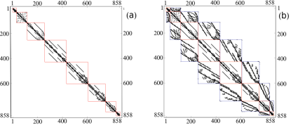
Figure 1: (Color online): Hamiltonian matrix written in the $|\gamma_{i}\rangle$ basis. (a) Block structure of the Hamiltonian in the non-interacting case, for the system $N/L=7/4$, with parameter $F_{r=1}=0.25$. Since $N=7$ the matrix contains $8$ blocks corresponding to the $N+1$ manifolds. The intra-manifold off diagonal couplings are set by the hopping terms that do not couple $\gamma_{i}$ states with different manifold number. (b) Tight-binding-type many-body Hamiltonian matrix for the same parameter from panel (a). The other parameters are: $\Delta_{g}=1.61$, $J_{a}=0.082$, $J_{b}=-0.13$, $C_{0}=-0.094$, $C_{\pm 1}=0.037$, and $C_{\pm 2}=-0.0022$.

and $\langle\psi_{M^{\prime}}|\psi_{M}\rangle=\delta_{M,M^{\prime}}$. The off-diagonal blocks are not square matrices but their dimension is $d_{M}\times d_{M+1}$. They are computed from the single-particle exchange term

$$\hat{H}_{M,M^{\prime}}\equiv\langle\psi_{M^{\prime}}|\sum^{L}_{l=1}\omega_{B}C_{0}\left(\hat{a}^{\dagger}_{l}\hat{b}_{l}+h.c.\right)|\psi_{M}\rangle.$$ (9)

By choosing $\langle\gamma_{i};M|\psi\rangle=1/\sqrt{d_{M}}$ we obtain a simplified tight-binding-type Hamiltonian for the manifolds

$$\hat{H}^{\prime}_{r}\simeq\sum^{N}_{M=0}\varepsilon^{r}_{M}|\psi_{M}\rangle\langle\psi_{M}|+\omega_{B}C_{0}(|\psi_{M}\rangle\langle\psi_{M+1}|+h.c.),\;\;\;$$ (10)

where $\varepsilon^{r}_{M}=(\Delta_{g}-\omega_{B}r)M+(J_{a}-J_{b})M$, and $\tilde{\omega}_{B}\equiv\omega_{B}C_{0}\sqrt{M+1}$. Here we used the relation $N=N_{a}+N_{b}$, with $M\equiv N_{b}$, and the order of the resonance is approximately given by $r\approx\Delta_{g}/\omega_{B}$. To obtain the Hamiltonian (10) we have assumed that there is no additional relevant subclass of Fock states in any $M$-subspace, and all possible single-particle processes are equally probable. Under this condition, the Hamiltonian (10) averages over hopping and dipole-like transition processes, and its final dimension is just $N+1$. A different choice of the distribution of the coefficients $\langle\gamma_{i};M|\psi\rangle$ would lead to a similar effective Hamiltonian, but restricted to fewer participating states.

Interestingly, from the new Hamiltonian we can easily recognize an emerging localization of its respective eigenfunctions $|\phi\rangle$. To see this, we use $|\phi\rangle=\sum\nolimits_{M}Q_{M}|\psi_{M}\rangle$, which together with the Schrödinger equation, $\hat{H}^{\prime}_{r}|\phi\rangle=E|\phi\rangle$, yields the coefficient equation:

$$(E-\epsilon M)Q_{M}=\tilde{\omega}_{B}(Q_{M+1}+Q_{M-1}),$$ (11)

with $\;\;\epsilon=\Delta_{g}-\omega_{B}r+J_{a}-J_{b}$. This equation can be solved using the ansatz $Q_{M}=AJ_{M^{\prime}-M}(x_{B})$, where $x_{B}\equiv 2\omega_{B}C_{0}/\epsilon$ and $J_{M^{\prime}-M}(x_{B})$ is the Bessel function of the first kind. Therefore, by using the identity $2kJ_{k}(x)=x(J_{k+1}(x)+J_{k-1}(x))$ we find that the solution of Eq. (11) is: $E_{M}=\epsilon M$ and $|\phi_{M}\rangle=A\sum\nolimits_{M^{\prime}}J_{M^{\prime}-M}(x_{B})|\psi_{M^{\prime}}\rangle$, with $A$ being a normalization constant. In energy space the eigenfunction can be written as

$$\phi_{M}(\varepsilon)\equiv\langle\varepsilon|\phi_{M}\rangle=A\sum\nolimits_{M}J_{M^{\prime}-M}(x_{B})\psi_{M^{\prime}}(\varepsilon)$$ (12)

where $\psi_{M^{\prime}}(\varepsilon)$, the eigenfunctions of the Hamiltonian $\hat{H}^{\prime}_{r}(\tilde{\omega}_{B}=0)$, is a well-localized function around the energy $\varepsilon^{r}_{M}$. These functions clearly satisfy the relation $\psi_{M}(\varepsilon-\varepsilon^{r}_{M^{\prime}})=\psi_{M^{\prime}}(\varepsilon)$. These are Wannier-like functions in energy space. The probability density is then now given by

$$\frac{|\phi_{M}(\varepsilon)|^{2}}{|A|^{2}}=|J_{0}(x_{B})\psi_{M}(\varepsilon)+\sum_{M^{\prime}\neq M}J_{M^{\prime}-M}(x_{B})\psi_{M}(\varepsilon)|^{2},$$ (13)

which means that, for $x_{B}\ll 1$, the probability maximizes around the manifold energy $\varepsilon^{r}_{M}$. The condition for this to happen is to be far from the resonance where for typical system parameters: $2\omega_{B}C_{0}\ll\Delta_{g}-\omega_{B}r+J_{a}-J_{b}$ . At the resonance we have $\Delta_{g}\approx\omega_{B}r$ and $x_{B}\approx 1$, which implies an overlapping of neighbor manifolds, since the expansion coefficients in Eq. (13) with $|M^{\prime}-M|>0$ become non-negligible. This introduces a kind of hybridization effect between the manifolds responsible for the destruction of the strong localization of the eigenfunctions $\phi_{M}(\varepsilon)$ (see refs. IzrailevPhysSkripta2001 ; APolkovnikov2013 for other contexts of localization in energy space).

The energy gap between two neighboring manifolds characterizes the one-particle exchange process (see Fig. 3(b)) and can be estimated by straightforward diagonalization of the two-level Hamiltonian matrix

$$H^{r}_{2\times 2}=\left(\begin{array}[]{cc}\varepsilon^{r}_{M+1}&\omega_{B}C_{0}\\ \omega_{B}C_{0}&\varepsilon^{r}_{M}\\ \end{array}\right)\,,$$ (16)

from which we obtain

$$\Delta_{r}=\Delta_{g}\sqrt{\left(1-\frac{\omega_{B}r}{\Delta_{g}}+\frac{J_{a}-J_{b}}{\Delta_{g}}\right)^{2}+4\left(\frac{\omega_{B}C_{0}}{\Delta_{g}}\right)^{2}}.\;\;\;\;\;$$ (17)

We notice that the minimal energy range of the many-level spectrum is thus given by $\Delta E=N\Delta^{\rm min}_{r}$, with $\Delta^{\rm min}_{r}\approx 2\omega^{r}_{B}|C_{0}|$ and $\omega^{r}_{B}\equiv 2\pi F_{r}$ (for typical parameters, $\Delta_{g},\omega_{B}\gg|J_{b}-J_{a}|$). This energy scale is shown in Fig. 2(a) for the single-particle case ($N/L=1/10$).

II.4 Effects of the Interparticle Interaction

A more precise description of the many-body spectrum is obtained when considering the effects of the interactions, i.e., for $W_{a,b,x}\neq 0$. This induces a splitting of the internal manifold levels and couplings between the $|\gamma_{i}\rangle$ states. The coupling is strong especially at resonant tunneling condition (e.g. $F\approx F_{r}$). In this region, the manifold levels come closest (see Fig. 2(b)) and a natural mixing of the manifold states occurs, that is, the eigenstates of (1) become hybridized as explained in Sec. II.3. This latter effect is associated with the occurrence of avoided crossings (ACs) around $F_{r}$, i.e., with the lack of symmetries in the system CarlosThesis2013 . We can now easily estimate the largest manifold splittings generated by interparticle interaction. This is done by considering the basis states $\{|\gamma_{i}\rangle\}$ with $M$ particles sitting in a single-particle level, in one lattice site, for example $|\gamma_{i}\rangle\sim|N-M,0,..\rangle_{a}\otimes|M,0,...\rangle_{b}$. The energy cost due to the interaction strengths $W_{a,b,x}$ is thus given by

$$(U^{M}_{a})_{\rm max} = \frac{W_{a}}{2}(N-M)(N-M-1),$$

$$(U^{M}_{b})_{\rm max} = \frac{W_{b}}{2}M(M-1),$$

$$(U^{M}_{ab})_{\rm max} = 2W_{x}(N-M)M,$$ (18)

which allow one to compute the maximal intra-manifold splitting as $U(M)\equiv\max\{(U^{M}_{\beta=a,b})_{\rm max},(U^{M}_{ab})_{\rm max}\}$. We can also rewrite the width $\Delta E$ as follows

$$\Delta E=N\Delta^{\rm min}_{r}+U(N).$$ (19)

This expression is obtained by considering the maximal splitting of the highest manifold $M=N$, which occurs for those eigenstates, whose maximal projection in the $|\gamma_{i}\rangle$ space is given by the state with $N$ particles in the same upper-band level, say, the state $|\gamma_{i}\rangle\sim|000,...\rangle_{a}\otimes|N00,...\rangle_{b}$.

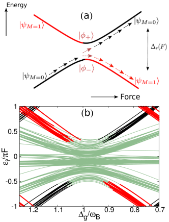
Figure 2: (Color online): (a) Numerically computed energy spectrum versus the Stark force in the single-particle case around $r=1$, with $N/L=1/10$. The inter-band coupling manifests itself around the resonance position $F_{r}$ by an avoided crossing. (b) Many-body spectrum for $N/L=4/5$, around $r=1$. The different color lines correspond to eigenstates of the type: $|\psi_{M=0}\rangle$ (black), $|\psi_{M=1}\rangle$ (red), and the mixed-like states, i.e., states with $0<M<N$ are represented by the green lines. In panel (a) $|\phi_{\pm}\rangle$ represent the hybridized states at $F=F_{r}$. The parameters are those of Fig. 1 with additional interaction strengths: $W_{a}=0.021$, $W_{b}=0.026$ and $W_{a}=0.023$.

In general, far from the resonance, any eigenstate of Eq. (1) can be rewritten in the dressed-like state basis $\{|M,\theta_{a},\theta_{b},\theta_{x}\rangle\}$ characterized by the integers $\theta_{\beta}=\langle\varepsilon_{i}|\sum\nolimits_{l}\hat{n}^{\beta}_{l}(\hat{n}^{\beta}_{l}-1)/2|\varepsilon_{i}\rangle$ and $\theta_{x}=2\langle\varepsilon_{i}|\sum\nolimits_{l}\hat{n}^{a}_{l}\hat{n}^{b}_{l}|\varepsilon_{i}\rangle$. The eigenenergies can then be approximated by

$$\varepsilon_{i}(M,\vec{\theta})\approx M_{i}\Delta_{r}+W_{a}\theta_{a,i}+W_{b}\theta_{b,i}+W_{x}\theta_{x,i}.$$ (20)

The mixing between the different $M$-manifolds in the presence of inter-particle interaction is now also triggered by the coupling between inter-manifold states with excess $\Delta M=\pm 2$. This fact implies that the Hamiltonian Eq. (10) contains a new term, which is just a second neighbor transition from the manifold $M$ to the manifold $M\pm 2$. This is nothing but an extended tight-binding model, with increasing on-site energies $\varepsilon_{i}(M,\vec{\theta})$. Therefore, even in the presence of weak interactions, the eigenstates $\langle\varepsilon|\phi_{M}\rangle$ preserves localization features.

Computing the following commutator

$$\left[\frac{\hat{H}}{\Delta_{g}},\hat{M}\right]=\sum\nolimits_{l,\mu}\frac{\omega_{B}C_{\mu}}{\Delta_{g}}\hat{a}^{\dagger}_{l+\mu}\hat{b}_{l}+\frac{W_{x}}{2\Delta_{g}}\hat{a}^{\dagger 2}_{l}\hat{b}^{2}_{l}-h.c.\;\;$$ (21)

shows that the transition from weak to strong mixing is determined by the competition between one- and two-particle exchange between the bands. This competition is the stronger the closer we are in resonance, at which we have that $\omega_{B}/\Delta_{g}\approx 1/r$. Furthermore, it is expected that for a filling factor $N/L\sim 1$, single- and two-particle transitions have the same occurrence probability, which makes the system strongly mixed. In the case $N/L\ll 1$, the dominant effect is a one-particle exchange characterized by the energy scale $\Delta_{r}$, and similarly for $N/L\gg 1$, the two-particle exchange process dominates with energy scale proportional to $W_{x}$. These two latter cases favor the weak manifold mixing. Therefore, the eigenstates of (1) are expected to be localized in energy space according to the effective Hamiltonian (10).

So far, we have studied the properties of the Hamiltonian (1) by using rather simple approximations based on the concept of manifold excitation. The results have shown to be in a good agreement with the numerical ones. We now show two direct consequences of the spectral properties; first we briefly describe the implementation of Landau-Zener-type dynamics by making the Stark force time-dependent. In this way, driving individual eigenstates $|\varepsilon_{i}\rangle$ across an avoided crossing may be straightforwardly implemented. Secondly, we study the connection between strong manifold mixing and quantum chaos in the resonant tunneling regime.

III Numerics: Landau-Zener Dynamics

Around a local resonance, our system provides a natural scenario for the study of Landau-Zener-type transitions. This can be done by defining a pulse $F(t)=F_{0}+\alpha t$, with $\alpha=\Delta F/\Delta T$. Here $\Delta F$ is the effective region of resonant tunneling and $\Delta T$ is the sweeping time. We focus on the dynamical driving of a state from the lowest manifold $|\psi_{M=0}\rangle$ for the single-particle case. We have then two manifolds $M=\{0,1\}$ and the spectrum of this system is shown in Fig. 1(a). We define the sweeping rate $\alpha$ using the Heisenberg relation $\Delta Td\approx 1$, where $d=\Delta E/\mathcal{N}_{s}=\Delta_{r}$ is mean level spacing at $F_{r}$.

The Hamiltonian is now time-dependent, $H(F(t))$, and the temporal evolution is computed by using a fourth-order Runge-Kutta method. In analogy with the LZ problem, the evolution across an avoided crossing can be diabatic, non-adiabatic and adiabatic. In the current case the dynamical regimes are determinated by the parameter $\lambda\equiv\alpha/d\,\Delta F$. Thus for $\lambda\ll 1$ we have slow driving through resonances, i.e., an adiabatic passage; for $\lambda\gg 1$ a diabatic one, also referred to as sudden quench, and for $\lambda\sim 1$ we have a non-adiabatic evolution.

To follow the evolution of a state across the RET regime, we compute the detection probabilities $p_{i}=|\langle\varepsilon_{i}|\hat{U}(t)|\psi(0)\rangle|^{2}$, where $\hat{U}(t)=\hat{\mathcal{T}}\exp\left[-i\int_{0}^{t}\hat{H}(F(t))dt\right]$. The distribution probability of the evolved wavefunction in the local energy space can be represented by means of the local density of states TDittrich1991 ; LFSantosPRL2012 :

$$P_{\psi}(\varepsilon,t)=\sum\nolimits_{i}p_{i}\delta(\varepsilon-\varepsilon_{i}),$$ (22)

with the delta function defined as

$$\delta(\varepsilon-\varepsilon_{i})=\lim_{\delta\rightarrow 0}\frac{1}{\pi}\frac{\delta}{(\varepsilon-\varepsilon_{i})^{2}+\delta^{2}}.$$ (23)

In figure 3 we show the evolution of the LDOS $P_{\psi}(\varepsilon,t)$ in the single particle case $N=1$, i.e. the Hamiltonian $\hat{H}^{\prime}_{r}$ in Eq. 10 is a $2\times 2$ matrix. The initial condition is $|\psi(0)\rangle\sim|100,...\rangle_{a}\otimes|000,...\rangle_{b}$, $M=0$. $|\psi(0)\rangle$ is evolved from $F_{0}<F_{r=1}$ to $F_{f}>F_{r=1}$ (left to right in Fig. 2(a)) for the two-state system $N/L=1/10$, and we can easily appreciate the different types of dynamics, that is: the left panel shows the adiabatic regime, for which $|\psi(0)\rangle$ nearly follows the energy path (see low-energy state in Fig. 2(a)) while being transformed into the excited state with $M=1$. This result is expected according to the exchange of character typical of an avoided crossing. This is a dynamical effect following from the adiabatic theorem, which was already experimentally probed in Arimondo’s group at Pisa University WimbPRL2009 ; Arimondo2011 ; NilsPRA ; Tayebirad2011 . On the other hand, the central panel shows the non-adiabatic transit for which the probability is split in both energy path. This effect is similar to the action of a beam splitter on an incident light beam. Finally the right panel depicts the diabatic passage for which the state does preserve its manifold number $M$ but not its energy path. This latter is characterized by the fidelity of the initial state, i.e. $|\langle\psi(0)|\hat{U}(t)|\psi(0)\rangle|^{2}\approx 1$.

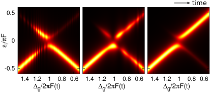
Figure 3: (Color online) Driving over the single particle spectrum in Fig. 2(a): Parametric-time evolution (from left to right) of a state initially prepared in the manifold $M=0$ (bottom left of the panels) across the resonance $r=1$, with the linear pulse $F(t)=F_{0}+\alpha t$. Dynamical parameters: (left) adiabatic transit ($\lambda=0.1$), (center) non-adiabatic transit ($\lambda=1$) and (right) diabatic transit ($\lambda=50$). The color scale is from black (small) to white (large), and $\delta=0.05$ in Eq. (II.4). The parameters are the same as in the previous figure.

IV Numerics: Interaction-induced quantum chaos

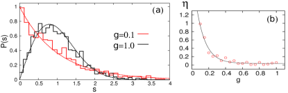
Figure 4: (Color online) Interaction effects: (a) The panel shows the level spacing distribution $P(s)$ for $N/L=6/5$ ($\mathcal{N}_{s}=1001$) for the interparticle control parameter $g=0.1$ (red/grey histogram, $\eta=0.97$) and $g=1.0$ (black histogram, $\eta=0.035$), and $W_{x}=W_{a}=W_{b}=0.025$. (b) Parameter $\eta$ as a function of $g$. The black line corresponds to an exponential fit. The reminding parameters are those of Fig. 2.

In this final section we study the static eigenspectrum at strong mixing conditions. Given the eigenenergies $\varepsilon_{i}$, the spectra can be analyzed by the use of random matrix measures Haakebook . A robust test of the universal properties of the discrete eigenspectrum is the so-called level spacing distribution $P(s_{i})$, where the spacing are defined as $s_{i}=(\varepsilon_{i+1}-\varepsilon_{i})/\langle s\rangle$. The spectrum must be unfolded in order to compare with the random matrix distributions, i.e., such that $\langle s_{i}\rangle=1$ (see ref. CarlosThesis2013 for details).

At the resonances $F_{r}$, the crossover between regular (Poisson), $P_{P}(s)=\exp(-s)$, and quantum chaotic (GOE) statistics, $P_{W}(s)=\pi s\exp(-\pi s^{2}/4)/2$, is reached by varying the inter-particle interaction. We define the parameter $g$, that allows one to tune the interaction, i.e., $W_{\beta,x}\rightarrow gW_{\beta,x}$. In the experiment this can be done via Feschbach resonances IblochREP2008 . As expected from the discussion in subsection II.4, for an energy band gap $\Delta_{g}\lesssim 1$ and $g=1$, all systems with $N/L\sim 1$ exhibit chaotic features characterized by the GOE distribution (see Fig. 4(a)-black). Nevertheless, this is not a general rule for every interaction strength, since for weakly interacting particles the manifold mixing becomes weaker. Hence quantum chaos can be tuned most easily by increasing the inter-particle interaction, for instance, $g=0\rightarrow 1$. To see this transition we compute the parameter

$$\eta=\frac{\int^{s_{0}}_{0}\left(P(s)-P_{W}(s)\right)ds}{\int^{s_{0}}_{0}\left(P_{P}(s)-P_{W}(s)\right)ds},$$ (24)

where $s_{0}=0.4729...$ is the intersection point between $P_{P}(s)$ and $P_{W}(s)$. We show the behavior of $\eta$ ($\eta=1$ for a poissonian case and $\eta=0$ for GOE) as a function of $g$ in fig. 4(b). We see that our two-band model allows us to concentrate a high density of many-body energy levels around a resonance, which induces the chaotic features of the system. This is not the case far from the resonant regime, since here the system is just weakly mixed due to the presence of the $M$-manifolds. Then the spectrum is nearly regular CarlosPRA2013 ; CarlosThesis2013 , and well characterized by the quantum numbers $M$ and $\vec{\theta}$ (see Sec. II.4), see Fig. 2(b).

We thus see that the mixing properties of our system allow for a straightforward identification of the onset of quantum chaos, which is a local effect in the plane $\varepsilon_{i}$ vs $F$. Nevertheless, a globally chaotic spectrum can also be reached by decreasing the energy bandgap $\Delta_{g}$ such that $gW_{x}/\Delta_{g}\sim 1$. In this case, not only resonant tunneling between two neighboring wells due to the Stark force is possible, but also via interaction MGreiner2011-0 ; InsbruckArxiv2013 . These two processes are equally relevant and, as immediate signature of this, the local resonances are destroyed. There are then avoided crossings in the entire energy spectrum. Therefore, we can switch from global to local quantum chaos by varying the bandgap $\Delta_{g}$.

V Conclusions

We studied the spectral properties of a many-body Wannier-Stark system, especially in the resonant tunneling regime. We showed that the main characteristics of our model are well described in terms of upper-band excitation subspaces, i.e., $M$-manifolds. This effective description provides an intuitive understanding of interaction-induced quantum chaos. Furthermore, we have shown that the knowledge of the spectral properties of the system allows us to control the dynamics when driving a simple two-state system across an avoided crossing, in the Landau-Zener framework LZ ; Arimondo2011 . Our system can be experimentally realized and it offers an interesting framework for future investigations of many-body physics PloetzJPB2010 ; PloetzEPJD2011 ; CarlosPRA2013 ; Oliver-1 ; InsbruckArxiv2013 .

VI Acknowledgments

We acknowledge financial support from the DFG (FOR760), the HGSFP (GSC 129/1) and the Institute for Theoretical Physics at Heidelberg University. It is our pleasure to warmly thank J. Madroñero for lively discussions. S.W. thanks furthermore the organizers of the workshop, L. Sirko and S. Bauch, and M. Kuś for his kind hospitality at the Polnish Academy of Sciences in Warsaw.

References

- (1) C. Kittel, Introduction to Solid State Physics (8th eddition), John Wiley Sons, Inc. (2005), p. 216.
- (2) Jaksch, D. and Bruder, C. and Cirac, J. and Gardiner, C. and Zoller, P. Phys. Rev. Let. 81, 15 (1998).
- (3) I. Bloch, J. Dalibard, and W. Zwerger, Rev. Mod. Phys. 80, 885 (2008).
- (4) M. Lewenstein, A. Sanpera, V. Ahufinger, B. Damski, A. Sen De, and U. Sen, Adv. Phys. 56, 243 (2007).
- (5) A. R. Kolovsky and A. Buchleitner, Phys. Rev. E 68 056213 (2003).
- (6) A. Tomadin, R. Mannella, and S. Wimberger, Phys. Rev. A 77, 013606 (2008).
- (7) A. Tomadin, R. Mannella, and S. Wimberger, Phys. Rev. Lett. 98, 130402 (2007).
- (8) A. Zenesini, H. Lignier, G. Tayebirad, J. Radogostowicz, D. Ciampini, R. Mannella, S. Wimberger, O. Morsch, and E. Arimondo, Phys. Rev. Lett. 103, 090403 (2009).
- (9) C. Sias, A. Zenesini, H. Lignier, S. Wimberger, D. Ciampini, O. Morsch, and E. Arimondo, Phys. Rev. Lett. 98, 120403 (2007); A. Zenesini, C. Sias, H. Lignier, Y. Singh, D. Ciampini, O. Morsch, R. Mannella, E. Arimondo, A. Tomadin, and S. Wimberger, New J. Phys. 10, 053038 (2008).
- (10) O. Morsch and M. Oberthaler, Rev. Mod. Phys. 78, 179 (2006).
- (11) E. Arimondo, D. Ciampini, A. Eckardt, M. Holthaus, and O. Morsch, Adv. At. Mol. Opt. Phys. 61, 515 (2012).
- (12) E. Arimondo and S. Wimberger, Tunneling of ultracold atoms in time-independent potentials, in Dynamical Tunneling, S. Keshavamurthy and P. Schlagheck (Eds.), Taylor Francis – CRC Press, Boca Raton (2011).
- (13) N. Lörch, F. Pepe, H. Lignier, D. Ciampini, R. Mannella, O. Morsch, E. Arimondo, P. Facchi, G. Florio, S. Pascazio, and S. Wimberger, Phys. Rev. A 85, 053602 (2012).
- (14) G. Tayebirad, A. Zenesini, D. Ciampini, R. Mannella, O. Morsch, E. Arimondo, N. Lörch, and S. Wimberger, Phys. Rev. A 82, 013633 (2010).
- (15) M. Gustavsson, E. Haller, M. J. Mark, J.G. Danzl, G. Rojas-Kopeinig and H.-C. Nägerl, Phys. Rev. Lett. 100, 080404 (2008); E. Haller, R. Hart, M. J. Mark, J. G. Danzl, L. Reichsöllner, and H.-C. Nägerl, Phys. Rev. Lett. 104, 200403 (2010).
- (16) O. Morsch, J.H. Müller, M. Cristiani, D. Ciampini, and E. Arimondo, Phys. Rev. Lett. 87, 140402 (2001).
- (17) M. Ben Dahan, E. Peik, J. Reichel, Y. Castin, and C. Salomon, Phys. Rev. Lett. 76, 4508 (1996).
- (18) S. R. Wilkinson, C. F. Bharucha, K. W. Madison, Qian Niu, and M. G. Raizen, Phys. Rev. Lett. 76, 4512 (1996).
- (19) P. Plötz, P. Schlagheck, and S. Wimberger, Eur. Phys. J. D 63, 47 (2011).
- (20) J. Simon, S. Bakr, M. Ruichao, M. E. Tai, M. Preiss and M. Greiner, Nature 472, 307 (2011).
- (21) F. Meinert, M. J. Mark, E. Kirilov, K. Lauber, P. Weinmann, A. J. Daley and H.-C. Nägerl, Phys. Rev. Lett. 111, 053003 (2013).
- (22) C. A. Parra-Murillo, J. Madroñero, and S. Wimberger, Phys. Rev. A 88, 032119 (2013).
- (23) C. A. Parra-Murillo, Ph.D. thesis, Heidelberg University, Heidelberg 2013.
- (24) P. Plötz, J. Madroñero, and S. Wimberger, J. Phys. B. 43, 08001(FTC) (2010).
- (25) W. S. Bakr, P. M. Preiss, M. E. Tai, M. Ruichao M, J. Simon, and M. Greiner, Nature 480, 500 (2011).
- (26) F. M. Izrailev, Phys. Scripta T 90, 95 (2001).
- (27) L. D’Alessio and A. Polkovnikov, Ann. of Phys. (N. Y.) 333, 19 (2013).
- (28) M. Glück, A. R. Kolovsky, and H. J. Korsch, Phys. Rep. 366, 103 (2002).
- (29) L. D. Landau, Phys. Z. Sowjetunion 2, 46 (1932); C. Zener, Proc. R. Soc. A 137, 696 (1932); E. C. G. Stückelberg, Helv. Phys. Acta 5, 369 (1932); E. Majorana, Nuovo Cimento 9, 43 (1932).
- (30) M. G. Bason, M. Viteau, N. Malossi, P. Huillery, E. Arimondo, D. Ciampini, R. Fazio, V. Giovannetti, R. Mannella, and O. Morsch, Nat. Phys. 8, 147 (2011); N. Malossi, M. G. Bason, M. Viteau, E. Arimondo, R. Mannella, O. Morsch, and D. Ciampini, Phys. Rev. A 87, 012116 (2013).
- (31) J. H. Shirley, Phys. Rev. 138, B979 (1965); Y. B. Zeldovich, Sov. Phys. JETP 24, 1006 (1967).
- (32) L. F. Santos, F. Borgonovi, and F.M. Izrailev, Phys. Rev. E 85, 036209 (2012).
- (33) T. Dittrich and U. Smilansky, Nonlinearity 4, 54 (1991).
- (34) F. Haake, Quantum signatures of chaos (Springer, Heidelberg, 2001).