Superdiffusion and Transport in $2d$-systems with Lévy Like Quenched Disorder

Abstract

We present an extensive analysis of transport properties in superdiffusive two dimensional quenched random media, obtained by packing disks with radii distributed according to a Lévy law. We consider transport and scaling properties in samples packed with two different procedures, at fixed filling fraction and at self-similar packing, and we clarify the role of the two procedures in the superdiffusive effects. Using the behavior of the filling fraction in finite size systems as the main geometrical parameter, we define an effective Lévy exponents that correctly estimate the finite size effects. The effective Lévy exponent rules the dynamical scaling of the main transport properties and identify the region where superdiffusive effects can be detected.

I Introduction

Transport and diffusion in highly heterogeneous random media is an interesting and complex phenomenon occurring in a wide class of materials, ranging from rocks to clouds, to engineered experimental samples PhysRevLett.65.2201 ; Davis:2002ys ; Benson:2001zr ; Palombo:2011mz ; Brockmann:2003uq ; PhysRevLett.72.203 ; PhysRevLett.54.616 . Matter or light typically crosses disordered regions with very different diffusion properties, so that the transport process can be described as a Lévy walk: motion consists of a sequence of scatterings followed by long jumps in the nonscattering regions. Two concurrent effects make the problem particularly hard: the quenched randomness, inducing correlation between displacements, and, if the material is heterogeneous on all scales, the typical broad distribution of the steps length, that can be heavy-tailed and Lévy distributed.

Tunable media with Lévy like properties Barthelemy:2008rt , reproducing all these effects, are an interesting testbed for the typically superdiffusive motion occurring in heterogeneous random materials. The ”Lévy” glasses are obtained by a packing of polydispersed glass spheres with Lévy distributed radii and embedded in a scattering matrix. As light is scattered only in the inter-sphere regions and freely travels ballistically inside the spheres, the propagation of light in these materials can be described as a correlated Lévy walk, with step length distribution $p(l)\sim l^{-(1+\alpha)}$, where the parameter $\alpha$ can be tuned by choosing an appropriate distribution of radii for the polydispersed spheres. In these systems, a superdiffusive behavior has been observed, with the characteristic length of the dynamical process growing as $\ell(t)\sim t^{1/z}$ with $z<2$.

A theoretical study of such systems is in general a non trivial task due to topological correlations between the step lengths: e.g. after crossing a large sphere a walker is likely backscattered in the same ballistic region. In this perspective, different theoretical and numerical approaches have been proposed barthelemy:2010PRE ; beenakker:2012 ; svenson:2013PRE . An analytic solution has been obtained for the simpler one dimensional case, the so called Lévy-Lorentz gas, corresponding to a packing of segments of Lévy distributed lengths separated by scattering centers PhysRevE.61.1164 ; in that case the dynamical exponent is $z=1+\alpha$ (superdiffusion) for $0<\alpha<1$ and $z=2$ (standard diffusion) for $\alpha>1$ Beenakker:2009ys ; Burioni:2010qy ; Burioni:2010fk ; Disanto . The regular and deterministic self similar version of the Lévy packings in higher dimension Buonsante:2011 have been recently introduced as basic geometrical models for quenched Lévy structures. Also in that case, numerical simulations show superdiffusion for $\alpha<1$ and standard diffusion for $\alpha>1$, with the dynamical exponent $z$ depending on $\alpha$, and very slightly on the dynamical rule and on the spatial dimension. Conversely, recent numerical results on $2$ and $3-$dimensional random sphere packings beenakker:2012 evidenced important differences with previous results. In particular superdiffusion was observed also for $\alpha>1$, i.e. for $\alpha\lesssim 1.6$. However, some aspects remained unclear, in particular the anomalous non monotonic behavior of $z$ as a function of $\alpha$, and the evaluation of the finite size effects beenakker:2012 . Notice that, for these random high dimensional heterogeneous models, even the definition of the packing procedure is a complex problem, still not understood from the theoretical point of view Biazzo:2009qy ; Parisi:2010 ; Torquato:2010 . What seems clear is that the dynamical behavior observed in all these Lévy quenched structures differs from the standard uncorrelated Lévy walk, where anomalous superdiffusion is present for $1<\alpha<2$ ann1 ; ann2 ; ann3 .

Another important point in the numerical experiments performed so far is that the samples are built by optimizing the packing, and minimizing the scattering region (optimal filling approach). In this way, the average distance between the spheres is kept constant as the system size grows, reproducing the behavior of deterministic fractals Buonsante:2011 . Within this prescription, the density of scatterers (or turbid fraction), for $\alpha<1$, becomes infinitesimal as the size goes to infinity, as one is building a so called slim fractal. Conversely, in the samples produced for the experiments Barthelemy:2008rt the turbid fraction is kept constant at different sizes even for $\alpha<1$, and this may give rise to important differences with respect the optimized Lévy structures of the theoretical approaches.

In this paper we first present an extensive numerical and theoretical analysis of two dimensional random packings of disks with radii distributed according to a Lévy law, and packed by minimizing the turbid fraction, i.e. with the optimal filling approach. Our results provide a new interpretation of the data found in beenakker:2012 . In particular, the anomalous non monotonic behavior of the dynamical exponent $z$ can be interpreted as a failure of the packing procedure in the regime $\alpha<0.5$. Moreover, numerical simulations show that in the thermodynamic limit of infinitely large samples the superdiffusive regimes observed for $1<\alpha\lesssim 1.6$ are expected to disappear and converge to a behavior similar to the deterministic case, where $z<2$ only for $\alpha<1$. In this framework we evidence that for $0.4\lesssim\alpha\lesssim 1.6$ strong finite size effects characterize the dynamics, the radii distribution and the packing procedure. We define the exponent $\alpha_{eff}$, describing such geometrical preasymptotic behavior, and we show that $\alpha_{eff}$ can be used for an effective description of the size effects characterizing the dynamics of realistic finite samples. Finally, we discuss the effect on the dynamics of the scattering length and of the truncation of the radii distribution.

Then, in order to make contact with the experiments, we consider the case of disks packing obtained by keeping the filling fraction constant at all scales, instead of minimizing the turbid fraction. This analysis evidences that, for any value of $\alpha$, as the size of the systems grows, the dynamical exponent $z$ becomes closer to 2, and we infer that the system is experiencing a crossing from a superdiffusive to a diffusive regime, with a large crossover region where superdiffusive effects can appear. The evidence is corroborated by analyzing the response of the dynamical exponents to the change of the scattering mean free path length and the fixed filled fraction $f$. We remark that such a crossover from ballistic to diffusive behavior is also present in the case where all the spheres have the same radius singler .

The outline of the work is as follows. In Section II we introduce the dynamics and the optimized packing procedure. In Section III we study the geometrical properties of the samples, introducing the effective exponent. We then show the results of our dynamical simulations and scaling effects in Section IV. Finally, Section V is devoted to the simulations at fixed filling, designed to make contact with the experiments. Section VI contains our conclusions.

II Random Lévy packings and dynamics

The packing algorithm follows the work of Beenakker et al. beenakker:2012 and the parameters of the random Lévy structure are:

• $N$, the number of disks (spheres);

• $L_{x},\,L_{y}$ the thickness and the width of the slab, respectively;

• $r_{min}$ and $r_{max}$, the minimum and the maximum radii, respectively;

• $\beta$, the exponent used to generate the radii distribution, featuring a power law $p(r)\sim r^{-(1+\beta)}$. We set $\alpha=\beta-d+1$, with $d=2$ in the case of disks.

The latter distribution is sampled following the recursive formula beenakker:2012 :

$$r_{k}={} r_{\rm max}\left[1+\frac{k}{k_{\rm max}}(r_{\rm max}^{\beta}-1)\right]^{-1/\beta},$$ (1)

$$\;\;k=0,1,2,\ldots k_{\rm max},$$

generating the radii ordered by size from the largest to the smallest one. According to beenakker:2012 disks can be placed randomly in the systems avoiding overlaps. The filling fraction $f$ at size $L$ is defined as the ratio between the total volume of the disks placed in the sample, $V_{D}(L)$, and the total volume $V(L)$ of the sample:

$$f(L)=\frac{V_{D}(L)}{V(L)}.$$ (2)

The complementary of $f$ is the turbid fraction $\phi(L)=1-f(L)$, that is, the system volume fraction occupied by the scatterers.

We introduce two different packing procedures illustrated in the Top Panel of Fig. 1. In the first, the newly added disk is approached to its closest neighbor, in the second it is also rotated around the neighboring disk until it is still not overlapping with the rest of the systems 0953-8984-16-37-002 ; Packing_Xu . The results of this new procedures are reported in Fig. 1 (bottom panel). The data clearly show that both prescriptions give the same qualitative result, presenting only a small improvement in the filling fraction. Therefore, hereafter, we adopt the original procedure which is the less demanding from a computational point of view. An example of a Lévy disks packing produced by this algorithm is found in Fig. 3.

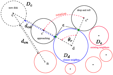
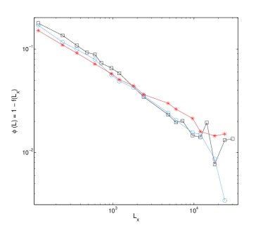
Figure 1: (Color online) (Top Panel) The geometric outline of the two methods implemented. When a new disk with center $c$ is placed, the program searches for the closest neighbor among the close disks (the disk with the $d$ center in this case). The distance between them is computed and the disk moved to a $\epsilon$ distance placing it in $c^{\prime}$ (close packing prescription, $\epsilon$ randomly chosen from a flat distribution in the $(10^{-4},1/4)\cdot r_{min}$). In the drop and roll method we further move the new disk rotating it around the closest neighbor until it touches an existing disk close to it. (Bottom Panel) Turbid fraction from the simulations at optimized filling following the three prescription presented: random packing (squares), dense packing prescription (circles) and the drop and roll algorithm (asterisks). The curves correspond to $\alpha=0.4$.

We then implement the specific dynamics of transport in the Lévy packing. The rays of light experience a ballistic motion inside the disks and an isotropic Poisson process in between the spheres, i.e. in the turbid region.

In particular, at each move we extract a random direction and a random step length $s$ from the distribution

$$P(s)ds=\frac{1}{\lambda}\exp{(-s/\lambda)}ds,$$ (3)

being $\lambda$ the scattering mean free path. If the ray crosses one or more disks, the actual step length has to be incremented until the ending point belongs to the turbid region and the new step length becomes $l=s+\bar{s}$ ($\bar{s}$ is the spaced covered within the disks). An example of a trajectory is shown in Fig. 2.

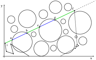
Figure 2: (Color online) An example of a trajectory: the single step length $s$ extracted from Eq. (3) is the length that the ray covers outside the disks between two scattering events. The distance covered within them is not taken into account. In this figure the extracted length is $s=\bar{ia}+\bar{bc}+\bar{df}$, while the actual step length is $l=\bar{if}$ due to the time spent by the ray within the disks. The latter is $\bar{s}=\bar{ab}+\bar{cd}$, so that $l=s+\bar{s}$.

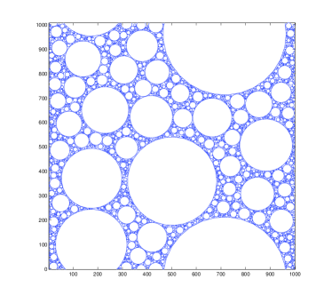
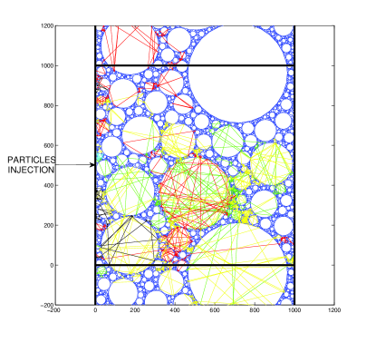
Figure 3: (Color online) (a) A Lévy glass with $L_{x}=L_{y}=10^{3}$, $r_{max}=250$, $\alpha=0.4$ and $N_{disk}=4\cdot 10^{3}$. The geometry is constrained on the $x=0$ and $x=L_{x}$ boundaries, while the $y=[0,L_{y}]$ ones are periodic; (b) The dynamics on the same sample. The program injects particles into the $x=0$ surface and let them diffuse until they reach the opposite side of the slab or they are backscattered to $x=0$. The original cell is framed with solid black line. The periodic bounds allow the motion to continue over the $y=0$ and $y=L_{y}$ borders.

In the transmission simulations we select the initial point on the $x=0$ side of the slab. The particles then walk as long as they reach the opposite side of the slab ($x=L_{x}$) or until they are backscattered to the $x=0$ surface (see Fig. 3). For the measure of the probability distribution $P(r,t)$ and of the mean square displacement, we pack the disks with periodic boundary conditions and the starting point is chosen randomly in the turbid fraction.

We let the maximum radius range from $r_{max}=10$ to $r_{max}=1500$, with $L_{x}=R_{S}r_{max}$ ($R_{S}=6$) and $L_{y}=4L_{x}$. The number of disks ranges from few hundreds at small system sizes to $\sim 6\cdot 10^{7}$. We initially choose $\lambda=r_{min}=1$. For each transmission run we simulate $5\cdot 10^{6}$ rays, while in the mean square displacement and $P(r,t)$ runs only $10^{5}$ rays are simulated, due to the time-consuming computation of the single ray trajectory.

III The filling fraction and the effective $\alpha$ exponent

Let us now consider the behavior of the filling and turbid fraction. Figure 4 describes, in our packing, the turbid fraction as a function of $L$. In large $L\to\infty$ systems we evidence that: for $\alpha\lesssim 0.5$, $\phi(L)$ goes to a constant; in the intermediate regimes $0.5\lesssim\alpha\lesssim 1.6$, $\phi(L)$ vanishes at large size with a characteristic exponent that we call $\alpha_{exp}$, i.e. $\phi(L)\sim L^{\alpha_{exp}-1}$; finally for $\alpha\gtrsim 1.6$, $\phi(L)$ goes to a constant in the large $L$ limit. We remark that the behavior of $\phi(L)$ is here more complex than that observed in deterministic self similar Lévy structuresBuonsante:2011 . In that case, the packing is regular, exact and it is built by a recursive procedure. There, $\phi(L)\sim L^{\alpha-1}$ for $\alpha<1$ and $\phi(L)$ goes to a constant for $\alpha>1$, defining the so called slim and fat fractals, respectively.

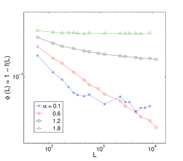
Figure 4: (Color online) The numerical behavior of $\phi(L)$ as a function of $L$ for $\alpha=0.1$ (asterisks), $\alpha=0.6$ (squares), $\alpha=1.2$ (circles), $\alpha=1.8$ (triangles).

Another useful quantity for the description of the packing properties is the average distance $\epsilon$ between two spheres (see Fig. 7 inset). We assume that, on the average, around each sphere there is a turbid region whose thickness $\epsilon(L)$ can depend on the system size $L$. This quantity is related to the turbid fraction by:

$$1-f(L)=\frac{\epsilon(L)A(L)}{V(L)}f(L)$$ (4)

where $A(L)$ is the average surface of the spheres.

The ratio $A/V$ as a function of the systems size is independent of the packing algorithm, and can be evaluated directly from the sphere distribution Eq. (1). In particular, if $k_{max}$ is large enough, the effect of discretization is negligible, and we can set $p(r)\sim r^{-(1+\beta)}$. We have therefore:

$$A_{c}(d,r_{max}) = C_{A}(d)\int_{1}^{r_{max}}{r^{d-1}p(r)dr}$$

$$V_{c}(d,r_{max}) = C_{V}(d)\int_{1}^{r_{max}}{r^{d}p(r)dr}.$$ (5)

where $C_{A}(d)$ and $C_{V}(d)$ are the constants defining the surface and the volume, respectively, at a given dimension $d$ (for instance $C_{A}(2)=2\pi$ and $C_{V}(3)=4/3\pi$). We finally obtain:

$$\frac{V}{A}\left(r_{max}\right)=\frac{C_{V}(d)}{C_{A}(d)}\frac{r_{max}^{-\alpha+1}-1}{r_{max}^{-\alpha}-1}\frac{-\alpha}{-\alpha+1}.$$ (6)

From this equation, we find in the thermodynamic limit

$$\frac{V}{A}\left(L\to\infty\right)\propto\left\{\begin{array}[]{ll}L^{-\alpha+1}&\textrm{if $0<\alpha<1$}\\ const&=\frac{C_{V}(d)\alpha}{C_{A}(d)(\alpha-1)}\qquad\textrm{if $1<\alpha$}\end{array}\right.$$ (7)

as $r_{max}$ si related to the system size $L$, by $L=r_{max}\cdot R_{S}$. Formulas (4) and (7) evidence that for $\alpha<1$ if the average distance between the disks is kept constant, then the turbid fraction is vanishing with the system size.

We now compare in Fig. 5 $V/A(L)$ as found by using our simulations, and the analytical results of Eq. (6), showing also the thermodynamic limit $L\to\infty$ as found in Eq. (7). Fig. 5 evidences that the sampling correctly reproduces the analytical form of $V/A(L)$. However, for $0.05\lesssim\alpha\lesssim 0.4$ and for $0.6\lesssim\alpha$, this ratio grows differently with respect to the expected asymptotic behaviour. This means that the finite system displays an effective exponent $\alpha_{eff}\neq\alpha$.

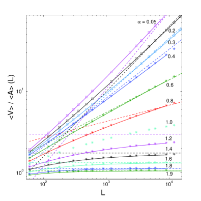
Figure 5: (Color online) The comparison of $V/A(L)$: the experimental results (squares and asterisk), the analytic function (solid line) and the $L\to\infty$ limit (dashed line) as found for $0.05\leq\alpha\leq 1.9$. The discrete sampling reproduces correctly the analytical result. We also note that, for $0.05\lesssim\alpha\lesssim 0.4$ and for $0.6\lesssim\alpha\lesssim 1.8$ we are in a pre-asymptotic range, and the $V/A$ ratio has not converged yet to the expected value. In particular, for low $\alpha$ finite size effects overestimate the value of the exponent while at large $\alpha$ the value is underestimated.

The value of $\alpha_{eff}$ as a function of the scale $L$ can be easily calculated by the logarithmic derivative of Eq. (6):

$$1-\alpha_{eff}=\frac{d}{d\ln L}\ln\frac{V}{A}(L)=(1-\alpha)\frac{1}{1-L^{\alpha-1}}+\alpha\frac{L^{-\alpha}}{L^{-\alpha}-1}.$$ (8)

The function is plotted in Fig. 6, showing that for $\alpha<0.5$ finite size effects overestimate the value of the exponent ($\alpha_{eff}>\alpha$), while for $\alpha>0.5$ we have $\alpha_{eff}<\alpha$.

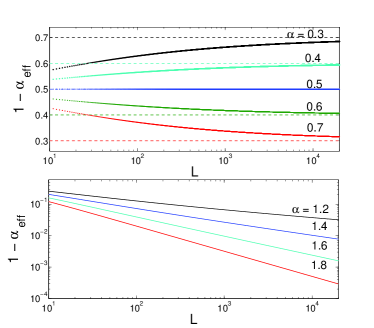
Figure 6: (Color online) (top) The $1-\alpha_{eff}(L)$ curves for $0<\alpha<1$. Note that for $\alpha<1/2$ we find $\alpha_{eff}>\alpha$ while $\alpha_{eff}<\alpha$ for $\alpha>1/2$. For $\alpha=0.5$ we have $\alpha_{eff}=\alpha$ for every $L$. In all the other case the $1-\alpha_{eff}(L)$ functions slowly converge to the asymptotic limit $1-\alpha$ (dashed lines). (bottom) The $1-\alpha_{eff}(L)$ curves for $1<\alpha<2$. Again, we found slow convergence to the asymptotic limit $1-\alpha_{eff}=0$.

Let us now evaluate $\epsilon(L)$ as defined in Eq. (4), estimating the average surface, the volume of disks and the filling fraction $f$ in our packing simulations. In Fig. 7 we plot $\epsilon(L)$ for the $0.05\leq\alpha\leq 1.8$ range. $\epsilon(L)$ diverges for $\alpha\lesssim 0.5$. This implies that the packing is not working, since at large values of $L$ one is not able to keep a constant distance between the disks. Therefore, the average turbid region between particles has a linear size greater than the scattering length $\lambda$, so that the light ray will pass more time in the scattering region, slowing down its dynamic. On the other hand, $\epsilon(L)$ seems to be constant ($\epsilon\sim 0.4$) for $\alpha\gtrsim 0.5$. This suggests a real packing with limited space between disks. In the intermediate regime $\alpha\simeq 0.4-0.5$, $\epsilon(L)$ display large oscillations evidencing an instability in the packing procedures. We notice that this crossover region corresponds to the value $\alpha=0.5$ where $\alpha_{eff}$ as a function of $L$ change its behavior (see figure 6).

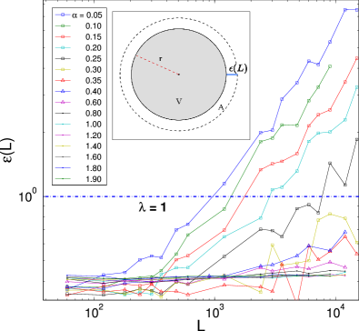
Figure 7: (Color online) Numerical data evidence that $\epsilon(L)$ depends on the system size $L$. Each line refers to a different $\alpha$ in the $0.1\leq\alpha\leq 1.8$ range which is displayed from top (dark grey squares $\alpha=0.1$) to bottom (squares, triangles and dots). The function diverges only for $\alpha\lesssim 0.5$, while at higher $\alpha$ it is constant. The horizontal dashed line denoted the scattering length $\lambda=1$. (Inset) On average, around each sphere there is an empty region whose thickness is defined to be $\epsilon$, the filling fraction $f$ is related to $\epsilon$ and the average volume $V$ and surface $A$ according to formula (4).

From this plot, it is clear that the region $\alpha\lesssim 0.5$, featuring an anomalous dynamical behavior in beenakker:2012 , does not correspond to a real packing and should be excluded from our measures. On the other hand, once $\alpha$ exceeds the $\sim 0.4-0.5$ threshold, $\epsilon(L)$ appears to be constant, so the $(1-f)/f$ term in Eq. (4) has to decrease as $A/V(L)$. It is then reasonable to compare $\alpha_{exp}$, coming from the direct measure of the turbid fraction from packing simulations, with $\alpha_{eff}$ obtained in theoretical analysis. In the regime where $\epsilon(L)$ is almost constant we should find $\alpha_{exp}\sim\alpha_{eff}$. In Fig.8 we present the results of this analysis evidencing a good agreement.

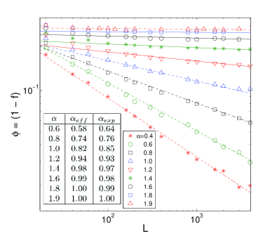
Figure 8: (Color online) The fitted $\phi(L)$ curves giving the $\alpha_{exp}$ exponents.
(Inset) The comparison between the two exponents $\alpha_{eff}$ and $\alpha_{exp}$ as found for different $\alpha$ in Fig. 8.

The general picture seems now quite clear. Although we choose the disks radii according to a certain $\alpha$ (or a $\beta=\alpha+d-1$), at finite size the packing features a different self similar structure: there exists another exponent $\alpha_{eff}$ which effectively drives the geometrical scaling since the thermodynamic limit has not been reached yet. Moreover, the mean thickness $\epsilon$ of the turbid region around each sphere has two different behavior for $0.1\leq\alpha<0.5$ and $0.5\leq\alpha<2$, respectively. In the first range, $\epsilon$ diverges giving rise to an anomaly in the system topology, and signaling that the packing fails. On the other hand, when $0.5\leq\alpha<2$, $\epsilon$ is almost constant. This in turn results in the comparable values of the two exponents $\alpha_{exp}$ and $\alpha_{eff}$, driving the scaling of $\phi\propto L^{\alpha_{exp}-1}$ and $\frac{V}{A}(L)\propto L^{1-\alpha_{eff}}$. The exponent $\alpha_{eff}$ is therefore the true geometrical parameter related to the effective packing.

IV Transport in $2d$ random Lévy packings

IV.1 The total transmission

The first quantity we measure in simulations at optimal filling is the transmitted intensity for different system thicknesses. A ray of light starts from the $x=0$ surface and diffuses according our dynamics until it comes back at the $x=0$ (reflection), or it reaches $x=L_{x}$ (transmission). We then count the number $r_{t}(L_{x})$ of rays that cross the slab on the total number of rays $r(L_{x})$ and we obtain the transmitted intensity $T(L_{x})=r_{t}(L_{x})/r(L_{x})$. Repeating the simulation and varying the thickness of the slab, we eventually find the $T(L_{x})$ function. We expect to find a scaling of the transmitted probability $T(L_{x})$ function, with now $L_{x}=L$ following the scaling relation Burioni:2010fk ; Buonsante:2011 :

$$T(L)\propto\frac{1}{L^{(z-1)}}.$$

In Fig. 9 we plot the resulting $T(L)$ for $\alpha=0.2$, in the region where packing fails and the distance between disks increases with the size. Clearly, there are two different ranges of the size where both the turbid fraction and the transmission probability behave differently. For low thickness range ($L\in[60,650]$) the algorithm succeeds in filling the system and, in fact, the turbid fraction decreases as a power law with $L$. Inside this interval, the packing works and the transmission probability scales with a super-diffusive exponent $z=1.47$ (much lower than the $z=2$ expected for a diffusive regime). Then, for $L>650$, the turbid fraction stops lowering with increasing size and the system presents an almost constant turbid fraction, i.e. $f\sim 0.96$. In this regime, the transmission probability behaves differently as well. We find indeed that the scaling exponent governing the $T(L)$ becomes closer to the diffusive case $z=2$. The same qualitative behavior characterizes the whole range $\alpha\in[0.0,0.4]$.

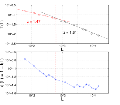
Figure 9: (Color online) $\alpha=0.2$: (Top) the $T(L)$ function with the two different interpolating lines (squares and circles for the experimental points and the fitting solid lines): squares for the low thicknesses range and circles for the higher ones. (Bottom) The $1-f(L)$ (turbid volume) function (asterisks). The delimiting thickness $L_{D}\sim 650$ is enlightened with the vertical dashed line.

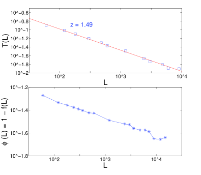
Figure 10: (Color online) $\alpha=0.6$: (Top) The $T(L)$ function (squares) with the scaling interpolation (solid line). (Bottom) The $1-f(L)$ (turbid volume) function (asterisks).

As we can see in Fig. 10, outside this problematic range we eventually find a power law decrease of the turbid fraction in the whole range of $L$ we analyzed. In Fig. 11 we show the transmitted intensity for $0.4\leq\alpha<2$. The fitting curves gives the values for $z$ that are resumed in the inset of Fig. 11, in the anomalous range the value of the exponent increases, due to the failure of the packing procedure. The plot agrees very well with that presented for the $2d$ case in beenakker:2012 .

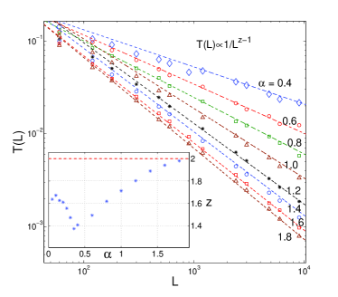
Figure 11: (Color online) The transmitted intensity $T(L)$ scaling with system size $L$ for different $\alpha$ value. The fit of the function gives the exponent $z-1$. (Inset) The dynamic exponent $z$ (asterisks) as a function of $\alpha$. Here, we merged the $z$ found in the anomalous range $0.1\leq\alpha\leq 0.4$. The diffusive limit $z=2$ (dashed line) is shown.

IV.2 The Time resolved transmission

The next dynamical quantity we analyze is the time-resolved transmission. The parameters of the simulations are identical to the ones outlined before. The transmission (or backscatter) time of each particle is recorder and binned in a histogram, and the time resolved transmission should follow the scaling form:

$$T(t,L)=L^{\eta}\tilde{f}(L/l(t)),$$ (9)

while the $P(r,t)$ the probability function, should scale as

$$P(r,t)=l^{-1}(t)f(r/l(t)).$$ (10)

We are now able to evaluate both scalings, as the growth of the characteristic length is related to the total transmission by the Einstein relation Burioni:2010fk ; cates $l(t)\propto t^{1/z}$ and $\eta=1-2z$. As we show in Fig. 12, the scaling picture holds for both for $P(r,t)$ and $T(L,t)$, evidencing a nice data collapse at least at large enough $L$.

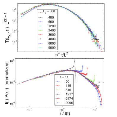
Figure 12: (Color online) (a) Scaling of time-resolved transmission $T(L,t)$ for $\alpha=1.2$ and different slab thicknesses. The characteristic length is set to $L^{z}$, as in Eq. (9). (b) Scaling of the average probability $P(r,t)$ for the system with $\alpha=0.8$ and $L={r_{m}ax}\cdot R_{S}=6\cdot 10^{3}$. The spikes stem from the ballistic motion inside the bigger disks and they disappear as soon as $t\gtrsim r_{max}$. The scaling pictures holds in the whole time range analyzed, satisfying the scaling hypothesis made in Eq. (10). The characteristic length has been set to $l(t)=t^{1/z}$, being $z$ the dynamical exponent governing the transmitted intensity.

IV.3 Scaling and the effective $\alpha$ exponent

Our simulations confirm the results in beenakker:2012 that superdiffusive anomalous transmission is observed for $0.5\lesssim\alpha\lesssim 1.6$, at variance with the deterministic self-similar models of Lévy packings, where super-diffusive behavior occurs only for $\alpha<1$ Buonsante:2011 . Interestingly, in the same regime $0.5\lesssim\alpha\lesssim 1.6$ our static study evidences that, for finite size systems, the filling fraction is not described by the exponent $\alpha$ characterizing the radii distribution $p(r)\sim 1/r^{d+\alpha}$ but an effective size dependent exponent $\alpha_{eff}$ has to be introduced. We, therefore, expect that also the transport properties may be affected by the finite size of the system.

We now calculate the exponent $z$ for different values of $L$. In particular, we estimate $z(L)$ by fitting consecutive intervals of the $T(L)$ function separately. For example, the fitting of $T(L)$ in the $60\leq L\leq 400$ range provides the value of $z$ at the average length of the analyzed range $L=230$. In Fig. 13 we show the results of this analysis.

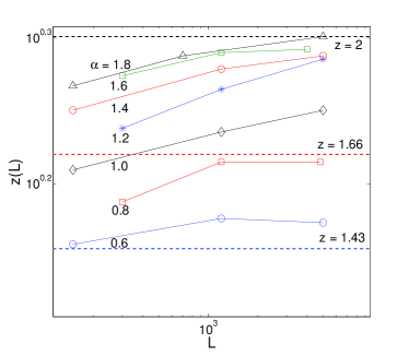
Figure 13: (Color online) The $z(L)$ function. The data refer to the $\lambda=1$ and $0.6\leq\alpha\leq 1.8$ simulations. The $z$ suggested by the ansatz $z=2/(2-\alpha)$ ($\alpha<1$) and the diffusive limit $z=2$ ($\alpha\geq 1$) are shown for comparison (dashed lines). While the exponents found for $\alpha<1$ seem to stop their rise with $L$, for $\alpha\geq 1$ they slowly grow toward $z=2$. The latter is reached only by the $\alpha=1.8$ set (black triangles) at the largest system size analyzed.

In general $z(L)$ features a growth with the system size and its limit is consistent with the value $z=2$ for $\alpha>1$, while for $\alpha<1$ also in the extrapolated infinite size regime a superdiffusive $z$ seems to persists. This behavior at large $L$ is similar to the case of the deterministic Lévy fractals. We notice that in the simulation in Buonsante:2011 , due to the deterministic rule used to build the fractals, much larger systems can be considered and finite size effects are in general negligible.

At finite size, it is therefore reasonable to study the exponent $z$ as a function of the effective exponent $\alpha_{eff}$ characterizing the finite size packing, and compare this function with the one found in Buonsante:2011 on a deterministic packing. Let us recall that in that work $z(\alpha)$ follows the heuristic ansatz $z=2/(2-\alpha)$ in the $0<\alpha\leq 1$ range, while $z=2$ for $\alpha>1$. In Fig. 14 we show that indeed $z(\alpha_{eff})$ is well approximated by this ansatz ($z=2/(2-\alpha)$ is also plotted in Fig. 13). The diffusive regime $z=2$ is reached only when $\alpha_{eff}\to 1$, recovering the distinction between a superdiffusive and diffusive regime below and above $\alpha=1$ respectively. Our analysis have been performed in the $2d$ case, but we expect this phenomenology to hold also in $3d$ systems.

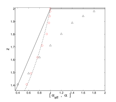
Figure 14: (Color online) The comparison between $z(\alpha_{eff})$ (circles), and $z(\alpha)$ (triangles). The $1D$ analytical result $z=\alpha+1$ (black solid line) and the ansatz $z=\frac{2}{2-\alpha}$ (black dashed line) are also shown. The $z(\alpha)$ significantly differs from the deterministic fractals case ansatz and from the $1D$ analytical result. Once we consider $\alpha_{exp}$ as the system characteristic exponent, the dynamical exponents $z$ appear to recover the curve found in the deterministic fractals case.

IV.4 The scattering mean free path

The dynamical exponents in the truly asymptotic regime, at infinite size, do not change by varying the scattering mean free path $\lambda$. However it is not clear what is the role of $\lambda$ in a regime where preasymptotic effects determine the dynamical behavior at finite sizes. Here, we will show that the results obtained in previous sections, at least at large $L$, are robust with respect to a variation of the scattering mean free path. We remark that we set $\lambda=1=r_{min}$ as in beenakker:2012 . However, in the experiments $r_{min}=2.5\mu m$ and $\lambda=12\mu m$, thus corresponding to $\lambda\sim 5$ in our setup.

Parameters	$\lambda=10$	$\lambda=1$	$\lambda=0.1$
$\alpha=0.8$	$1.61$	$1.64$	$1.64$
$\alpha=1.0$	$1.76$	$1.78$	$1.79$
$\alpha=1.2$	$1.89$	$1.90$	$1.97$

Table 1: The dynamical exponents $z$ found by varying $\lambda$.

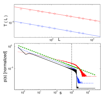
Figure 15: (Color online) (top) The transmission probability for $\lambda=0.1$ (squares) and $\lambda=10$ (circles) for $\alpha=1.0$. The fitting lines are reported, giving $z=1.76$ and $z=1.79$ for the $\lambda=10$ and $\lambda=0.1$ respectively. We fitted taking into account the largest system sizes to avoid, especially in the $\lambda=10$ case, the multi-disks crossing events to influence the $T(L)$ estimation. (bottom) The $p_{s}(s)$ single step length probability function for $\lambda=0.1$ (solid line), $1$ (dashed line) and $10$ (dotted line). All the sets are for $\alpha=1.0$, $L_{x}=6\cdot 10^{3}$ and $R_{S}=6$. The dot-dashed line shows the expected $p_{(}s)\sim s^{-(\alpha+1)}$ for comparison.

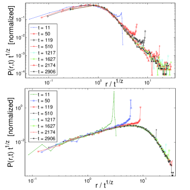
Figure 16: (Color online) (top) The scaling of $P(r,t)$ as from the simulation with $\lambda=0.1$, $\alpha=1.2$ and $L=r_{max}\cdot R_{S}=6\cdot 10^{3}$. The scaling length is set to $l(t)=t^{1/z}$ with $z(\alpha=1.2)=1.94$; (bottom) The same function has been plotted for the system featuring $\lambda=10$. Here $z(\alpha=1.2)=1.93$.

We analyze the system response to a variation of $\lambda$, keeping $R_{S}=6$, and $\alpha=[0.8,1.0,1.2]$ and averaging over $5\cdot 10^{6}$ initial conditions. Our fits at large $L$ show that $z$ does not change switching from $\lambda=0.1$ to $10$ and remains in good agreement with the case $\lambda=1$ (see Table (1)) though there is, of course, a drop in the transmission probability $T(L)$ (see Fig. 15 upper panel). As we can see in Fig. 16 the scaling of the $P(r,t)$ works in both cases, $\lambda=0.1$ and $\lambda=10$ once the characteristic length $l(t)$ is taken into account.

The main differences at varying $\lambda$ regard the frequency of multi-disks crossing events and they are evidenced in Fig. 15, lower panel, by inspecting the single step length distribution $p_{s}(s)$. We note indeed that the bump, found for $\lambda=1$ in the range $1\lesssim s\lesssim 20$, disappears for $\lambda=0.1$. This is a clear indication that we are isolating the chord distribution of the disks, avoiding multi-disks crossing. We remark that the average distance between the spheres in our packing is $\epsilon\simeq 0.4$ (see Figure 7) and multi-disks crossing is completely avoided only for $\lambda\ll\epsilon$. On the contrary, for $\lambda=10$ the bump spreads over the whole step size range, even further than $s\sim r_{max}$. Here the multi-disks crossing events are the leading process within the slab. The signal dies very slowly and we cannot distinguish a range where $p_{s}(s)$ follows the chords distribution function. This is at variance with the $\lambda=[0.1,1]$ systems, where a sharp cut-off is present at the $s\sim 2r_{max}$ length.

IV.5 The truncation length

As a last check of the lengths involved in our model, we consider explicitly the effects of truncation in the radii distribution i.e. of the parameter $R_{S}$. We run an additional set of simulations for $R_{S}=[2,\,4,\,6]$, maximized $f$, $\lambda=1.0$ and $0.4\leq\alpha\leq 2.8$;

In Table (2) we show the results for the effective exponent $\alpha_{eff}$ evidencing that systems with different $R_{S}$ features the same $\alpha_{eff}$ i.e. they are equivalent from a geometrical point of view. We then compute the transmission properties. The resulting $z$ are shown in Table (3).

$R_{S}$/$\alpha$	$0.4$	$0.6$	$0.8$	$1.0$	$1.2$	$1.4$	$1.6$	$1.8$
$2$	$0.54$	$0.62$	$0.74$	$0.85$	$0.92$	$0.95$	$0.98$	$0.99$
$4$	$0.53$	$0.66$	$0.78$	$0.86$	$0.96$	$0.98$	$0.99$	$1.00$
$6$	$0.56$	$0.64$	$0.76$	$0.85$	$0.93$	$0.97$	$0.98$	$1.00$

Table 2: The $\alpha_{eff}$ exponents found for different $R_{S}$.

$\alpha$	$z$ ($R_{S}=2$)	$z$ ($R_{S}=4$)	$z$ ($R_{S}=6$)
$0.4$	$1.43$	$1.36$	$1.41$
$0.6$	$1.49$	$1.52$	$1.55$
$0.8$	$1.55$	$1.65$	$1.65$
$1.0$	$1.67$	$1.77$	$1.76$
$1.2$	$1.72$	$1.90$	$1.91$
$1.4$	$1.70$	$1.94$	$1.93$
$1.6$	$1.72$	$1.96$	$1.96$
$1.8$	$1.75$	$1.98$	$2.00$

Table 3: The resulting dynamical exponents $z$ for the $L=2r_{max}$ ($R_{S}=2$) and $L=4r_{max}$ ($R_{S}=4$) cases compared with the $R_{S}=L/r_{max}=6$ case.

The dynamical exponents $z$ seem to be independent of the truncation for $R_{S}>2$, while a discrepancy is found for what concerns the data at $R_{S}=2$ especially in the regime of large $\alpha$ i.e. $\alpha>0.8$. In particular, the dynamical exponent $z$ referring to $R_{S}=2$ is found to be smaller than the one computed for $R_{S}=6$ and $R_{S}=4$. We remark that for $R_{S}=2$ the diameter of the largest sphere equals the system size $L$, and direct ballistic transmission becomes much more likely. Nevertheless, Fig. 17 evidences that even for $R_{S}=2$ the scaling scheme for the probability distribution $P(r,t)$ holds using the proper characteristic length $l(t)=t^{1/z}$.

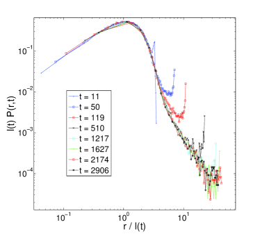
Figure 17: (Color online) Scaling of the $P(r,t)$ function for a $R_{S}=2$ sample with $L=2000$ and $\alpha=1.0$. The characteristic length is $l(t)=l^{1/z}$. The spikes correspond to the ballistic motion within the largest disk in the slab. The latter is now as large as the slab itself.

V Lévy Packings at fixed filling

The experimental setup described in Barthelemy:2008rt presents an important difference with respect to our simulations IV. The theoretical packings, in order to reproduce a fractal sampling, try to maximize the filling fraction $f$, i.e. the number of disks in the slab. On the opposite, in the experiments the filling fraction is kept constant, in particular $f=71\%$. Therefore, in the experiment, $\alpha$ only affects the step length distribution, but plays no role in the behavior of $f$ passing from one system scale to another. Recalling the packing procedure, we notice that if the term $(1-f)/f$ in Eq. (4) is constant with respect to $L$, then at $\alpha<1$ the packing features a diverging sphere-to-sphere distance $\epsilon(L)$. We then expect to observe a diffusive behavior as the size $L$ grows, since the diffusive region becomes dominant. However, at finite size the average spacing $\epsilon$ between the spheres can be comparable to $\lambda$, and this could give rise also in this case to an effective exponent $z$ smaller than 2, since at that scale the underlying disks distribution display a fractal superdiffusive geometry.

For this purpose we now analyze finite size effects in a system with fixed $f=0.7$, varying $\lambda=[0.1,1.0,10]$ and $\alpha=[0.8,1.0,1.2]$. To construct a slab with fixed $f$, we increment the number of disks until we reach the desired value of $f$. The disk are then placed randomly according the usual algorithm. We found that $f\sim 0.7$ is a filling fraction value that can be easily reached at all the system sizes and for all the $\alpha$ exponents, so that the samples are created very quickly. We simulated the walk of $5\cdot 10^{6}$ particles, analyzing the transmission properties of the system. The geometry is still fixed to $R_{S}=6$ and $r_{min}=1$.

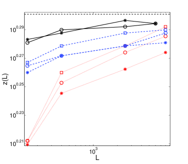
Figure 18: (Color online) The evaluation of $z(L)$ for system with $f_{fix}=0.7$. The data refer to $\lambda=10$ (dotted lines), $\lambda=1$ (dashed lines) and $\lambda=0.1$ (solid lines). The system exponents are $\alpha=0.8$ (asterisks), $\alpha=1.0$ (circles) and $\alpha=1.2$ (squares) respectively. The $z(L)$ found for $\lambda=[1,10]$ seems to converge to the exponents found in the $\lambda=0.1$ case, which is almost constant over the whole range. The black dashed line shows the diffusive limit $z=2$.

We test the scaling with the system size by measuring $z(L)$ obtained by fitting $T(L)$ on different $L$-intervals. The results are plotted in Fig. 18. The $z$ exponent is converging to the diffusive case as the system size increases. Furthermore, the data from $\lambda=1$ and $\lambda=10$ undergo a rapid growth, whereas the $\lambda=0.1$ exponent is slowly increasing, as if it has already reached the diffusive case. However, all the exponents seem to converge to a common $z$ value, very close to the diffusive $z=2$.

The results obtained at the maximum size $L=1.2\cdot 10^{4}$ are summarized in Table 4. The data confirm that the convergence to $z=2$ is faster for smaller values of $\lambda$. For instance, in the case $\alpha=0.8$ we find $z=1.86$ and $z=1.97$ for $\lambda$ set to $10$ and $0.1$, respectively. Moreover, if we lower the filling fraction $f_{fix}$ to $0.5$, $\epsilon(L)$ is, obviously, growing faster with the system size and the dynamics converges more rapidly to a diffusive regime.

Parameters		$f_{fix}=0.7$	$f_{fix}=0.5$
$\lambda=10$	$\alpha=0.8$	$1.86$	$-$
′′	$\alpha=1.0$	$1.94$	$-$
′′	$\alpha=1.2$	$1.97$	$-$
$\lambda=1$	$\alpha=0.8$	$1.92$	$1.97$
′′	$\alpha=1.0$	$1.95$	$1.97$
′′	$\alpha=1.2$	$1.94$	$1.96$
$\lambda=0.1$	$\alpha=0.8$	$1.97$	$-$
′′	$\alpha=1.0$	$1.96$	$-$
′′	$\alpha=1.2$	$2.00$	$-$

Table 4: The dynamical exponents found by maximizing $f$ ($f_{max}$ column) and by fixing it ($f_{fix}$) columns.

It is then very likely that we are observing a crossing between a superdiffusive and diffusive regime. The latter could be driven by a characteristic length of the system that, so far, is unknown. This length could depend on the scattering mean free path, the truncation length, the average disks-to-disk distance (our $\epsilon$) and on the system exponent $\alpha$ as well, so that the most general form of this length should be $\Lambda(\alpha,f,\epsilon)$. As we demonstrated, it is reasonable to expect that decreasing the $\lambda$ length and-or decreasing the $f_{fix}$ value, one should lower this length, so to observe at lower sizes the crossing from a superdiffusive to a diffusive regime. The behaviour of the system is outlined in Fig. 19. We start with a Lévy packing whose thickness is equal (or of the same order) of the scattering mean free path. Obviously, transport properties follow a ballistic behavior, as the whole slab is crossed with few jumps. As we increase the system size, we turn the ballistic behavior in a super-diffusive one until the slab thickness is of the same order the characteristic length $\Lambda(\alpha,f,\epsilon)$. We are probably evaluating our dynamic exponents in this central size range, as they converge to the diffusive case $z=2$ when decreasing $\lambda$ (i.e. when we decrease $\Lambda$, thus anticipating the crossing). From there on, the system undergoes an additional crossing to a diffusive case, where the correct, diffusive exponent is recovered.

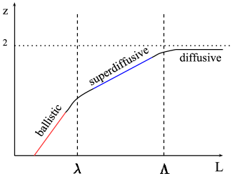
Figure 19: (Color online) The hypothetical convergence of the dynamical exponent $z$ to a diffusive case as we increase the system size.

As a last step for the fixed filling case, we consider explicitly the effect of the building procedure of the actual samples, that limits $L$ to be the double of $r_{max}$, i.e.$R_{S}=2$. We run an additional set of simulations: $R_{S}=[2,\,4,\,6]=L/r_{max}$, fixed $f=0.7$, $\lambda=1.0$ and $0.4\leq\alpha\leq 2.8$; and we compute the transmission properties. We recover the same behaviour as that found in the case of optimized filling. In the Table 5 we resume the resulting dynamical exponents. Again, we find good agreement between the $R_{S}=[4,\,6]$ configurations, while the $R_{S}=2$ systems are not converging to the diffusive limit $z=2$ since the truncation length is as large as the system size.

$\alpha$	$z$ ($R_{S}=2$)	$z$ ($R_{S}=4$)	$z$ ($R_{S}=6$)
$0.4$	$1.89$	$1.94$	$-$
$0.6$	$1.82$	$1.91$	$-$
$0.8$	$1.82$	$1.98$	$1.92$
$1.0$	$1.84$	$1.92$	$1.95$
$1.2$	$1.80$	$1.98$	$1.94$
$1.4$	$1.75$	$-$	$-$
$1.6$	$1.80$	$-$	$-$

Table 5: The resulting dynamical exponents $z$ for the $L=2r_{max}$ ($R_{S}=2$) and $L=4r_{max}$ ($R_{S}=4$) cases compared with the $R_{S}=L/r_{max}=6$ case. The data refer to the $f_{fix}=0.7$ case.

VI Conclusions

Building a tunable medium with given superdiffusive properties is an extremely interesting task. It can help to unravel the effect of quenched disorder in presence of large fluctuations and it gives access to the engineering of disordered media with desired transport effectsBarthelemy:2008rt . Besides, it can also allow to extract valuable information on transport and diffusion in natural porous media PhysRevLett.65.2201 ; Palombo:2011mz . A self similar geometry with a Lévy like step length distribution in a wide range appears to be the crucial ingredient to obtain the desired superdiffusive effects. A packing obtained at fixed filling fraction can present a self similar region in a restricted sizes window but at larger sizes it will turn towards a diffusive sample.

In this paper, we have analyzed in details a $2-$dimensional packing of disks with Lévy distributed radii and we studied the finite size effects arising from the complex polydispersed disks packing. We have evidenced that the behavior of the filling fraction at varying system size can be used as a key parameter for the scaling property of the total transmission and for the time resolved transmission. The packing at finite size features an effective step length distribution whose parameter $\alpha_{eff}$ is different from the initial $\alpha$ extracted from the disks radii self similar distribution. Superdiffusive effects are then observed when $\alpha_{eff}<1$. Interestingly, the exponent $z$ of the scaling length $l(t)=t^{1/z}$ as a function of $\alpha_{eff}$ is consistent with the ansatz found in deterministic packings, a result that certainly deserves further investigations.

- (1) A. Ott, J. P. Bouchaud, D. Langevin, and W. Urbach, Phys. Rev. Lett. 65, 2201 (1990).
- (2) A. B. Davis and A. Marshak, Journal of the Atmospheric Sciences 59, 2713 (2002).
- (3) Benson, David A. and Schumer, Rina and Meerschaert, Mark M. and Wheatcraft, Stephen W., Transport in Porous Media 42, 211 (2001).
- (4) M. Palombo, A. Gabrielli, S. de Santis, C. Cametti, G. Ruocco, and S. Capuani, J. Chem. Phys. 135, 034504 (2011).
- (5) D. Brockmann and T. Geisel, Phys. Rev. Lett. 90, 170601 (2003).
- (6) F. Bardou, J. P. Bouchaud, O. Emile, A. Aspect, and C. Cohen-Tannoudji, Phys. Rev. Lett. 72, 203 (1994).
- (7) T. Geisel, J. Nierwetberg, and A. Zacherl, Phys. Rev. Lett. 54, 616 (1985).
- (8) P. Barthelemy, J. Bertolotti, and D. S. Wiersma, Nature (London) 453, 495 (2008).
- (9) P. Barthelemy, J. Bertolotti, K. Vynck, S. Lepri and D. S. Wiersma, Phys. Rev. E 82, 011101 (2010).
- (10) C. W. Groth, A. R. Akhmerov, and C. W. J. Beenakker, Phys. Rev. E 85, 021138 (2012).
- (11) T. Svensson, K. Vynck, M. Grisi, R. Savo, M. Burresi and D.S. Wiersma, Phys. Rev. E 87, 022120 (2013).
- (12) E. Barkai, V. Fleurov, and J. Klafter, Phys. Rev. E 61, 1164 (2000).
- (13) R. Burioni, L. Caniparoli, and A. Vezzani, Phys. Rev. E 81, 060101 (2010).
- (14) R. Burioni, S. di Santo, S. Lepri and A. Vezzani, Phys. Rev. E 86, 031125 (2012).
- (15) R. Burioni, L. Caniparoli, S. Lepri, and A. Vezzani, Phys. Rev. E 81, 011127 (2010).
- (16) C.W.J. Beenakker, C.W. Groth and A.R. Akhmerov, Phys. Rev. B 79, 024204 (2009).
- (17) P. Buonsante, R. Burioni, and A. Vezzani, Phys. Rev. E 84, 021105 (2011).
- (18) I. Biazzo, F. Caltagirone, G. Parisi, and F. Zamponi, Phys. Rev. Lett. 102, 195701 (2009).
- (19) G. Parisi and F. Zamponi, Rev. Mod. Phys. 82, 789 (2010).
- (20) S. Torquato and F. H. Stillinger, Rev. Mod. Phys. 82, 3197 (2010).
- (21) T. Geisel, J. Nierwetberg and A. Zacherl, Phys. Rev. Lett. 54, 616 (1985).
- (22) M. F. Shlesinger, G. M. Zaslavski and J. Klafter, Nature (London) 363, 31 (1993).
- (23) G. Zumofen and J. Klafter, Phys. Rev. E 47, 851 (1993).
- (24) T. Svensson, K. Vynck, E. Adolfsson, A. Farina, A. Pieri and D.S. Wiersma, arXiv:1310.6419v1 (2013).
- (25) T. Okubo and T. Odagaki, Journal of Physics: Condensed Matter 16, 6651 (2004).
- (26) N. Xu, J. Blawzdziewicz, and C. S. O’Hern, Phys. Rev. E 71, 061306 (2005).
- (27) M.E. Cates J. Phys. (Paris) 46, 1059 (1985).