Controlling the level of sparsity in MPC

Abstract

In optimization routines used for on-line Model Predictive Control (MPC), linear systems of equations are usually solved in each iteration. This is true both for Active Set (AS) methods as well as for Interior Point (IP) methods, and for linear MPC as well as for nonlinear MPC and hybrid MPC. The main computational effort is spent while solving these linear systems of equations, and hence, it is of greatest interest to solve them efficiently. Classically, the optimization problem has been formulated in either of two different ways. One of them leading to a sparse linear system of equations involving relatively many variables to solve in each iteration and the other one leading to a dense linear system of equations involving relatively few variables. In this work, it is shown that it is possible not only to consider these two distinct choices of formulations. Instead it is shown that it is possible to create an entire family of formulations with different levels of sparsity and number of variables, and that this extra degree of freedom can be exploited to get even better performance with the software and hardware at hand. This result also provides a better answer to an often discussed question in MPC; should the sparse or dense formulation be used. In this work, it is shown that the answer to this question is that often none of these classical choices is the best choice, and that a better choice with a different level of sparsity actually can be found.

1 Introduction

Model Predictive Control (MPC) is one of the most commonly used control strategies in industry. Some important reasons for its success include that it can handle multi-variable systems and constraints on control signals and states in a structured way. In each sample, some kind of optimization problem is solved. In the methods considered in this paper, the optimization problem is assumed to be solved on-line. The optimization problem can be of different types depending on which type of system and problem formulation that is used. The most common variants are linear MPC, non-linear MPC and hybrid MPC. In most cases, the effort spent in the optimization problems boils down to solving Newton-system-like equations. Hence, lots of research has been done in the area of solving this type of system of equations efficiently when it has the special form from MPC. It is well-known that these equations (or at least a large part of them) can be cast in the form of a finite horizon LQ control problem and as such it can be solved using a Riccati recursion. Some examples of how Riccati recursions have been used to speed up optimization routines can be found in, for example, [9, 13, 8, 5, 15, 11, 2, 4, 1, 3, 6].

The objective with this paper is to revisit the recurring question in MPC whether the optimization problem should be formulated in a way where the states are present as optimization variables or in a form where only the control signals are the optimization variables. The latter is often called condensing. In general this choice in turn affects which type of linear algebra that is possible to use in the optimization routine. If the states are kept, the system of equations solved in each iteration in the solver potentially becomes sparse and if the condensed formulation is used this system of equations instead becomes dense. Since it is known that the computational complexity of the sparse formulation grows with the prediction horizon length $N$ as $\mathcal{O}(N)$ if sparsity is exploited while the computational complexity for the dense one grows as $\mathcal{O}(N^{3})$, the sparse one is often recommended for problems with large $N$ and the dense one is often recommended for problems with small $N$. In this paper, it will be shown that this choice does not have to be this binary. It is shown that it is possible to construct equivalent problems that have a level of sparsity in between these two classical choices, but also to increase the sparsity even further for certain types of problems. By using the approaches proposed in this work, formulations that are even more computationally efficient than the classical ones can be constructed.

The key to the performance improvement is that the proposed reformulations change the block-size of the sparse formulation. This makes it possible to tune this choice according the performance of the software and hardware available on-line. If a code generated solver is used, the selection of the most appropriate formulation of the problem can be done off-line in the code generation phase, taking the performance of the on-line hardware and software platform into account. Choosing a good, or even “optimal”, block-size is not a new idea in numerical linear algebra. See, e.g., [16]. However, it has, to the best of our knowledge, not previously been discussed for MPC and in particular not in the context of tailored linear algebra for MPC. Furthermore, the presented result hints that control engineers working with MPC should not ask themselves whether to formulate the problem in a sparse or dense way, but instead what is the correct level of sparsity for the problem at hand to obtain maximum performance which do not necessarily coincide with one of the two extreme choices that have been used classically.

In this article, $\mathbb{S}^{n}$ denotes symmetric matrices with $n$ columns. Furthermore, $\mathbb{S}_{++}^{n}$ ($\mathbb{S}_{+}^{n}$) denotes symmetric positive (semi) definite matrices with $n$ columns. The set $\mathbb{Z}_{++}$ denote the set of positive non-zero integers. A Sans Serif font is used to indicate that a matrix or a vector is, in some way, composed of stacked matrices or vectors from different time instants. The stacked matrices or vectors have a similar symbol as the composed matrix, but in an ordinary font. For example, $\mathsf{Q}=\operatorname{diag}(Q,\ldots,Q)$.

2 Problem formulation

The problem considered in this work is

$$\begin{array}[]{rl}{\underset{x_{t},u_{t}}{\text{min}}}&\hskip 2.84526pt\begin{aligned} \sum_{t=0}^{N-1}\frac{1}{2}\begin{bmatrix}x_{t}^{T}&u_{t}^{T}\end{bmatrix}\begin{bmatrix}Q_{t}&W_{t}\\ W_{t}^{T}&R_{t}\end{bmatrix}\begin{bmatrix}x_{t}\\ u_{t}\end{bmatrix}+\frac{1}{2}x_{N}^{T}Q_{N}x_{N}\end{aligned}\vspace{1ex}\\ \textrm{s.t.}&\hskip 2.84526pt\begin{aligned} x_{0}&=x^{0}\\ x_{t+1}&=A_{t}x_{t}+B_{t}u_{t},\;t=0,\ldots,N-1\\ 0&\geq H_{x,t}x_{t}+H_{u,t}u_{t}+h_{t},\;t=0,\ldots,N-1\\ 0&\geq H_{x,N}x_{N}+h_{N}\end{aligned}\end{array}$$ (1)

where the states $x_{t}\in\mathbb{R}^{n}$, the initial condition $x^{0}\in\mathbb{R}^{n}$, the control inputs $u_{t}\in\mathbb{R}^{m}$, the system matrices $A_{t}\in\mathbb{R}^{n\times n},B_{t}\in\mathbb{R}^{n\times m}$, the penalty matrices for the states $Q_{t}\in\mathbb{S}^{n}$, penalty matrices for the control inputs $R_{t}\in\mathbb{S}^{m}$, the cross penalty matrices $W_{t}\in\mathbb{R}^{n\times m}$, the state constraint coefficient matrix $H_{x,t}\in\mathbb{R}^{c\times n}$, the control signal coefficient matrix $H_{u,t}\in\mathbb{R}^{c\times m}$, the constraint constant $h_{t}\in\mathbb{R}^{c}$, and the prediction horizon $N\in\mathbb{Z}_{+}$. Moreover, the matrices $Q_{t}$, $R_{t}$ and $W_{t}$ are assumed to be chosen such that the following two assumptions are satisfied

Assumption 1

$R_{t}\in\mathbb{S}_{++}^{m}$

Assumption 2

$\begin{bmatrix}Q_{t}&W_{t}\\ W_{t}^{T}&R_{t}\end{bmatrix}\in\mathbb{S}_{+}^{n+m}$

Both constrained linear MPC problems and nonlinear MPC problems often boil down to solving problems similar to the one in (1) but without any inequality constraints during the Interior Point (IP) process or Active Set (AS) process, [9, 13, 8, 5, 15, 11, 2, 4, 1, 3, 6]. Hence, the ability of solving unconstrained versions of the problem in (1) efficiently is of great interest for the overall computational performance in the entire range of problems from simple unconstrained linear MPC problems, to nonlinear constrained and hybrid MPC problems.

As shown in [14], the problem in (1) can after a simple variable transformation be recast in an equivalent form with $W_{t}=0$. Therefore, the analysis in this work is restricted to the case when $W_{t}=0$ without any loss of generality.

Assumption 3

$W_{t}=0$

Remark 1

The results shown in this paper can easily be extended to common variants of MPC, e.g., problems where the control signal horizon differs from the prediction horizon, problems with affine system descriptions, as well as to reference tracking problems.

3 Classical optimization problem formulations of MPC

Traditionally, two optimization problem formulations of the MPC problem have been dominating in the MPC community. In the first formulation, the optimization problem in (1) with $W_{t}=0$ has been written more compactly as a Quadratic Programming (QP) problem in the form

$$\begin{array}[]{rl}{\underset{\mathsf{x},\mathsf{u}}{\text{min}}}&\hskip 2.84526pt\begin{aligned} \frac{1}{2}\begin{bmatrix}\mathsf{x}^{T}&\mathsf{u}^{T}\end{bmatrix}\begin{bmatrix}\mathsf{Q}&0\\ 0&\mathsf{R}\end{bmatrix}\begin{bmatrix}\mathsf{x}\\ \mathsf{u}\end{bmatrix}\end{aligned}\vspace{1ex}\\ \textrm{s.t.}&\hskip 2.84526pt\begin{aligned} \begin{bmatrix}\mathsf{A}&\mathsf{B}\end{bmatrix}\begin{bmatrix}\mathsf{x}\\ \mathsf{u}\end{bmatrix}&=\mathsf{b}\\ \begin{bmatrix}\mathsf{H}_{\mathsf{x}}&\mathsf{H}_{\mathsf{u}}\end{bmatrix}\begin{bmatrix}\mathsf{x}\\ \mathsf{u}\end{bmatrix}+\mathsf{h}&\leq 0\end{aligned}\end{array}$$ (2)

where $\mathsf{x}$, $\mathsf{u}$, $\mathsf{Q}$, $\mathsf{R}$, $\mathsf{q}$, $\mathsf{r}$, $\mathsf{b}$, $\mathsf{A}$, $\mathsf{B}$, $\mathsf{H}_{\mathsf{x}}$, $\mathsf{H}_{\mathsf{u}}$, and $\mathsf{h}$ are defined in the Appendix. Note that, $\mathsf{Q}$, $\mathsf{R}$, $\mathsf{A}$, $\mathsf{B}$, $\mathsf{H}_{\mathsf{x}}$, and $\mathsf{H}_{\mathsf{u}}$ are sparse matrices.

In the second formulation, the dynamics equations in (1) have been used to express $\mathsf{x}$ as

$$\mathsf{x}=S_{x,N}x_{0}+S_{u,N}\mathsf{u}$$ (3)

where $S_{x,N}$ and $S_{u,N}$ are defined in the Appendix. This expression can be used to eliminate the equality constraints containing the dynamics in the problem in (2). As a result, an equivalent problem can be derived in the form

$$\begin{array}[]{rl}{\underset{\mathsf{u}}{\text{min}}}&\hskip 2.84526pt\begin{aligned} &\frac{1}{2}\mathsf{u}^{T}\left(\mathsf{B}^{T}\mathsf{A}^{-T}\mathsf{Q}\mathsf{A}^{-1}\mathsf{B}+\mathsf{R}{}\right)\mathsf{u}-\left(\mathsf{B}^{T}\mathsf{A}^{-T}\mathsf{Q}\mathsf{A}^{-1}\mathsf{b}{}\right)^{T}\mathsf{u}\end{aligned}\vspace{1ex}\\ \textrm{s.t.}&\hskip 2.84526pt\begin{aligned} \left(\mathsf{H}_{\mathsf{x}}S_{u,N}+\mathsf{H}_{\mathsf{u}}{}\right)\mathsf{u}+\mathsf{h}+\mathsf{H}_{\mathsf{x}}S_{x,N}x_{0}\leq 0\end{aligned}\end{array}$$ (4)

where $\mathsf{B}^{T}\mathsf{A}^{-T}\mathsf{Q}\mathsf{A}^{-1}\mathsf{B}+\mathsf{R}$ is a dense matrix.

4 Quasi-sparse optimization formulations

As discussed in the introduction, many papers published on the subject illustrate that the sparse formulation in (2) is preferable over the dense one in (4) from a computational point of view. However, there also exists applications where the non-structure exploiting dense formulation turns out to be the fastest one. It can be realized both from the expressions for the analytical complexities as well as from numerical experiments that there are certain breakpoints in the problem sizes where one formulation is better than the other one. Traditionally, one rule-of-thumb is that the sparse formulation is faster for large values of $N$, and the dense one is faster for problems with small values of $N$. In this section it is discussed whether it is possible to do even better by combining ideas from these two traditional approaches. To reduce the complexity of the notation in the presentation, the ideas are illustrated on an MPC formulation where the system, penalties and constraints are independent of time.

4.1 Increasing the block-size

Partition the prediction horizon in $\tilde{N}+1$ subintervals with corresponding lengths $M_{k}\in\mathbb{Z}_{++}$, $k\in\{0,\tilde{N}\}$ with $\sum_{k=0}^{\tilde{N}}M_{k}=N+1$. To get a reformulated problem which is in the form of the one in (1) with a non-zero end penalty, the choice $M_{\tilde{N}}=1$ was made in this section. Define $\mathsf{x}_{k}=[x_{\tau_{k}+0}^{T}\,x_{\tau_{k}+1}^{T}\ldots x_{\tau_{k}+M_{k}}^{T}]^{T}$ and $\mathsf{u}_{k}=[u_{\tau_{k}+0}^{T}\,u_{\tau_{k}+1}^{T}\ldots u_{\tau_{k}+M_{k}-1}^{T}]^{T}$ where $\tau_{0}=0$ and $\tau_{k}=\sum_{i=0}^{k-1}M_{i},\;k>0$. Analogously to the equation in (3), given the state at a time $\tau_{k}$ and all control signals from subinterval $k$, all states in subinterval $k$ can be expressed as

$$\mathsf{x}_{k}=S_{x,M_{k}}x_{\tau_{k}}+S_{u,M_{k}}\mathsf{u}_{k}$$ (5)

and in particular we have that

$$x_{\tau_{k+1}}=x_{\tau_{k}+M_{k}}=A^{M_{k}}x_{\tau_{k}}+\begin{bmatrix}A^{M_{k}-1}B&A^{M_{k}-2}B&\ldots&B\end{bmatrix}\mathsf{u}_{k}\triangleq\mathsf{A}_{k}x_{\tau_{k}}+\mathsf{B}_{k}\mathsf{u}_{k}$$ (6)

Note that the equation in (6) is in state-space form. The new state dynamics describes the dynamics from the first sample in one condensed block to the first sample in the following block. Using these results, it is possible to write the sum of the stage costs for an entire subinterval as

$$\sum_{t=\tau_{k}}^{\tau_{k}+M_{k}-1}x_{t+1}^{T}Qx_{t+1}+u_{t}^{T}Ru_{t}=\begin{bmatrix}x_{\tau_{k}}^{T}&\mathsf{u}_{k}^{T}\end{bmatrix}\begin{bmatrix}\mathsf{Q}_{k}&\mathsf{W}_{k}\\ \mathsf{W}_{k}^{T}&\mathsf{R}_{k}\end{bmatrix}\begin{bmatrix}x_{\tau_{k}}\\ \mathsf{u}_{k}\end{bmatrix}$$ (7)

with

$$\begin{split}\mathsf{Q}_{k}&=S_{x,M_{k}}^{T}\cdot\operatorname{diag}\left(Q,\ldots,Q,0{}\right)\cdot S_{x,M_{k}},\\ \mathsf{W}_{k}&=S_{x,M_{k}}^{T}\cdot\operatorname{diag}\left(Q,\ldots,Q,0{}\right)\cdot S_{u,M_{k}},\\ \mathsf{R}_{k}&=S_{u,M_{k}}^{T}\cdot\operatorname{diag}\left(Q,\ldots,Q,0{}\right)\cdot S_{u,M_{k}}+\operatorname{diag}\left(R,\ldots,R{}\right)\end{split}$$ (8)

for $k\leq\tilde{N}-1$ and $\mathsf{Q}_{\tilde{N}}=Q$. As a result, the original problem can be re-cast in the form

$$\begin{array}[]{rl}{\underset{x_{\tau_{k}},\mathsf{u}_{k}}{\text{min}}}&\hskip 2.84526pt\begin{aligned} \sum_{k=0}^{\tilde{N}-1}\frac{1}{2}\begin{bmatrix}x_{\tau_{k}}^{T}&\mathsf{u}_{k}^{T}\end{bmatrix}\begin{bmatrix}\mathsf{Q}_{k}&\mathsf{W}_{k}\\ \mathsf{W}_{k}^{T}&\mathsf{R}_{k}\end{bmatrix}\begin{bmatrix}x_{\tau_{k}}\\ \mathsf{u}_{k}\end{bmatrix}+\frac{1}{2}x_{\tau_{\tilde{N}}}^{T}\mathsf{Q}_{\tilde{N}}x_{\tau_{\tilde{N}}}\end{aligned}\vspace{1ex}\\ \textrm{s.t.}&\hskip 2.84526pt\begin{aligned} x_{\tau_{0}}&=x^{0}\\ x_{\tau_{k+1}}&=\mathsf{A}_{k}x_{\tau_{k}}+\mathsf{B}_{k}\mathsf{u}_{k},\;k=0,\ldots,\tilde{N}-1\\ 0&\geq\mathsf{H}_{x,k}x_{\tau_{k}}+\mathsf{H}_{u,k}\mathsf{u}_{k}+\mathsf{h}_{k},\;k=0,\ldots,\tilde{N}-1\\ 0&\geq\mathsf{H}_{x,\tilde{N}}x_{\tau_{\tilde{N}}}+\mathsf{h}_{\tilde{N}}\end{aligned}\end{array}$$ (9)

with

$$\begin{split}\mathsf{H}_{x,k}&=\begin{bmatrix}H_{x}&0&\ldots&0&0\\ 0&\ddots&\ldots&0&0\\ 0&\ldots&0&H_{x}&0\end{bmatrix}S_{x,M_{k}}\in\mathbb{R}^{M_{k}c\times(M_{k}+1)n},\\ \mathsf{H}_{u,k}&=\begin{bmatrix}H_{x}&0&\ldots&0\\ 0&\ddots&\ldots&0\\ 0&\ldots&H_{x}&0\end{bmatrix}S_{u,M_{k}}+\begin{bmatrix}H_{u}&0&\ldots&0\\ 0&\ddots&\ldots&0\\ 0&\ldots&0&H_{u}\end{bmatrix}\in\mathbb{R}^{M_{k}c\times M_{k}m},\\ \mathsf{h}_{k}&=\begin{bmatrix}h\\ \vdots\\ h\end{bmatrix}\in\mathbb{R}^{M_{k}c},\;k=0,\ldots,\tilde{N}-1\\ \mathsf{H}_{x,\tilde{N}}&=H_{x},\;\mathsf{h}_{\tilde{N}}=h\end{split}$$ (10)

The new formulation can be interpreted as another MPC problem in the form in (1) with virtual prediction horizon $\tilde{N}$, virtual state dimension $\tilde{n}=n$, and the virtual control signal dimension for interval $k$ is $\tilde{m}=M_{k}\cdot m$. There are different variants of this formulation that give similar results. For example one can take $\mathsf{Q}_{\tilde{N}}=0$ and instead include the last state in the second last sub-interval. The number of inequality constraints in each virtual time step along the prediction horizon is $\tilde{c}_{k}=M_{k}\cdot c$ and the total number of inequality constraints is unaffected compared to the original problem. In words, this formulation partially condenses the original sparse problem into a new one where several original samples have been condensed into one new and are basically handled using the dense formulation. If $M_{0}=N$, roughly the traditional dense formulation in (4) is obtained and if $M_{k}=1,\;\forall k$, the traditional sparse one in (2) is obtained. Note that, the problems in (1) and in (9) are structurally identical and an algorithm (and an implementation of it) that can be applied to the problem in (1) can also be applied to the one in (9). Once the problem in (9) has been solved, $\mathsf{u}$ in Section 3 is directly obtained and the entire vector $\mathsf{x}$ can, if desired, easily be computed.

4.2 Decreasing the block-size

Consider a problem with diagonal $R$ and inequality constraints in the form

$$0\geq\begin{bmatrix}H_{x}&0\\ 0&H_{u}\end{bmatrix}\begin{bmatrix}x(t)\\ u(t)\end{bmatrix}+\begin{bmatrix}h_{x}\\ h_{u}\end{bmatrix}$$ (11)

where $H_{u}$ represents simple control signal constraints. Simple here means that the control signal constraints are, e.g., upper and lower bound constraints. For simplicity, we assume $H_{u}$ diagonal with diagonal elements $H_{u,k},k=1,\ldots,m$ in what follows. Note that, however, $H_{x}$ can be full as long as these state constraints do not involve control signals.

Partition the control signal $u_{t}$ in $M_{t}$ parts such that $u_{t}=\begin{bmatrix}u_{t,1}&u_{t,2}&\ldots&u_{t,M_{t}}\end{bmatrix}$ with $u_{t,k}\in\mathbb{R}^{m,\tilde{m}_{t,k}}$ and $B=\begin{bmatrix}b_{1}&b_{2}&\ldots&b_{M_{t}}\end{bmatrix}$, where $\tilde{m}_{t,k}\in\mathbb{Z}_{++}$, $t\in\{0,N-1\}$, $k\in\{1,M_{t}\}$ denotes the number of virtual control signals for which it holds that $\sum_{t=0}^{N-1}\sum_{k=1}^{M_{t}}\tilde{m}_{t,k}=Nm$. Then the state update equation can be written as

$$x_{t+1}=Ax_{t}+Bu_{t}=Ax_{t}+\sum_{k=1}^{M_{t}}b_{k}u_{t,k}$$ (12)

which can be equivalently reformulated, e.g., as

$$\begin{split}\tilde{x}_{t,2}&=A\tilde{x}_{t,1}+b_{1}u_{t,1}\\ \tilde{x}_{t,3}&=I\tilde{x}_{t,2}+b_{2}u_{t,2}\\ &\vdots\\ \tilde{x}_{t+1,1}&=I\tilde{x}_{t,M_{t}}+b_{M_{t}}u_{t,M_{t}}\end{split}$$ (13)

with some new states $\tilde{x}_{t,k}$ for which it holds that $\tilde{x}_{t,1}=x_{t},\;\forall t$. Since $R$ and $H_{u}$ are diagonal, the objective function and inequality constraints can be decomposed in $u(t)$ in an analogous way and the diagonal matrices corresponding to part $k$ are denoted $R_{k}$ and $H_{u,k}$, respectively. That in combination with the expression in (13), the problem in (1) can be reformulated in the form

$$\begin{array}[]{rl}{\underset{\tilde{x}_{k},\mathsf{u}_{k}}{\text{min}}}&\hskip 2.84526pt\begin{aligned} \sum_{k=0}^{\tilde{N}-1}\frac{1}{2}\begin{bmatrix}\tilde{x}_{k}^{T}&\mathsf{u}_{k}^{T}\end{bmatrix}\begin{bmatrix}\mathsf{Q}_{k}&\mathsf{W}_{k}\\ \mathsf{W}_{k}^{T}&\mathsf{R}_{k}\end{bmatrix}\begin{bmatrix}\tilde{x}_{k}\\ \mathsf{u}_{k}\end{bmatrix}+\frac{1}{2}\tilde{x}_{\tilde{N}}^{T}\mathsf{Q}_{\tilde{N}}\tilde{x}_{\tilde{N}}\end{aligned}\vspace{1ex}\\ \textrm{s.t.}&\hskip 2.84526pt\begin{aligned} \tilde{x}_{0}&=x^{0}\\ \tilde{x}_{k+1}&=\mathsf{A}_{k}\tilde{x}_{k}+\mathsf{B}_{k}\mathsf{u}_{k},\;k=0,\ldots,\tilde{N}-1\\ 0&\geq\mathsf{H}_{x,k}\tilde{x}_{k}+\mathsf{H}_{u,k}\mathsf{u}_{k}+\mathsf{h}_{k},\;k=0,\ldots,\tilde{N}-1\\ 0&\geq\mathsf{H}_{x,\tilde{N}}\tilde{x}_{\tilde{N}}+\mathsf{h}_{\tilde{N}}\end{aligned}\end{array}$$ (14)

with

$$\begin{split}\mathsf{A}_{k}&=\begin{cases}&A,\;k=0,M,2M,\ldots,(N-1)M\\ &I,\;\text{otherwise}\end{cases}\\ \mathsf{B}_{k}&=b_{\text{mod}(k,M)+1}\\ \mathsf{Q}_{k}&=\begin{cases}&Q,\;k=0,M,2M,\ldots,NM\\ &0,\;\text{otherwise}\end{cases}\\ \mathsf{R}_{k}&=R_{\text{mod}(k,M)+1}\\ \mathsf{H}_{x,k}&=\begin{cases}&\begin{bmatrix}H_{x}\\ 0\end{bmatrix},\;k=0,M,2M,\ldots,(N-1)M\\ &H_{x},\;k=\tilde{N}\\ &0,\;\text{otherwise}\end{cases}\\ \mathsf{H}_{u,k}&=\begin{cases}&\begin{bmatrix}0\\ H_{u,1}\end{bmatrix},\;k=0,M,2M,\ldots,(N-1)M\\ &H_{u,\text{mod}(k,M)+1},\text{otherwise}\end{cases}\\ \mathsf{h}_{k}&=\begin{cases}&\begin{bmatrix}h_{x}\\ h_{u,1}\end{bmatrix},\;k=0,M,2M,\ldots,(N-1)M\\ &h_{x},\;k=\tilde{N}\\ &h_{u,\text{mod}(k,M)+1},\;\text{otherwise}\end{cases}\end{split}$$ (15)

for the simplified case when the partitioning is done uniformly with a constant $M_{t}=M\in\left\{j\in\mathbb{Z}_{++}:m/j\in\mathbb{Z}_{++}{}\right\},\;\forall t$ over the prediction horizon. The reformulated problem can be interpreted as an optimization problem in the MPC form in (1) with virtual prediction horizon $\tilde{N}=NM$, virtual state dimension $\tilde{n}=n$, and virtual control signal dimension $\tilde{m}=m/M$. The number of inequality constraints is varying along the virtual prediction horizon, however, the total number of constraints is unchanged compared to the original problem. Once the problem in (14) has been solved, $\mathsf{u}$ and $\mathsf{x}$ in Section 3 are directly obtained.

Remark 2

Further degrees of freedom can be obtained by combining the approaches in Sections 4.1 and 4.2 by first decreasing the block-size and then increasing the block-size of the modified problem.

Remark 3

Note that, the ideas can also be applied to problems with similar structures. For example, to the moving horizon state-estimation problem and to the Lagrange dual of the optimal control problem.

5 Impact on a commonly used sparse linear algebra for MPC

The inequality constrained optimal control problems in (9) and (14) are usually either solved using either an interior point (IP) method or an active-set (AS) method. It is well-known that the main computational complexity in these algorithms can be formulated as solving a sequence of unconstrained variants of the original control problem. These problems in turn are solved by solving a linear system of equations corresponding to the KKT conditions of these unconstrained problems. This can be done in several ways. However, two commonly used approaches are to either use a Cholesky factorization applied to a problem where the states have been eliminated (commonly known as condensing) or a Riccati factorization applied to the problem where the states are kept as variables. If the problem is reformulated as described in Sections 4.1 and 4.2, it can be realized that the important block-sizes that appear in a sparse factorization will be changed. Even thought the Riccati factorization is used as an example in this work, it is expected that the proposed approaches in this work will have similar impact on other variants of sparse linear algebra used in MPC. However, none of the proposed reformulations will affect the dense formulation and the following (off-the-shelf) dense linear algebra. Hence, the focus in this section will be on how Riccati based sparse linear algebra is affected by the approaches introduced in this article. The required number of flops for the Cholesky factorization approach is known to be roughly $(Nm)^{3}/3$ and for the Riccati factorization it is roughly $N(1/3m^{3}+4n^{3}+4m^{2}n+6n^{2}m)$, [12]. A full specification of the Riccati approach used in this work can be found in [12, 1]. For simplicity, in this section it is assumed that the blocking is uniform non-time-dependent and that it is compatible with $N$ and $m$. In practice further improvements can potentially be achieved by using a non-uniform blocking factor. However, this also increases the complexity of determining a good one and it is therefore not clear whether it is worth that extra effort. Furthermore, it would also be possible to exploit and take into account in the complexity calculations the special structures in the reformulated problems. For example, the approach in Section 4.2 generates many sparse problem data matrices.

5.1 Increasing the block-size

The family of formulations achievable with this approach is parameterized by $M$, which will increase the block-size in the resulting sparse numerical linear algebra and make the formulation less sparse as $M$ grows. Since it holds that $\tilde{N}=N/M$, $\tilde{n}=n$, and $\tilde{m}=Mm$, the required number of flops for performing a Riccati factorization on the reformulated problem is $f_{1}(M)=N\left(M^{2}m^{3}/3+4n^{3}/M+4Mm^{2}n+6n^{2}m{}\right)$. The theoretical maximum possible gain in flops $f_{1}(1)/f_{1}(M^{*})$ which is independent of $N$ is illustrated in Figure 1 and can be found to be almost as much as a factor of $30$ in the considered problems. $M^{*}$ denotes the best choice of $M$ for given $n$ and $m$. Furthermore, note that, the relative improvement $f_{1}(1)/f_{1}(M)$ is independent of $N$. However, given an $N$ one can only select an $M\leq N$.

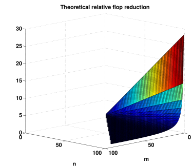
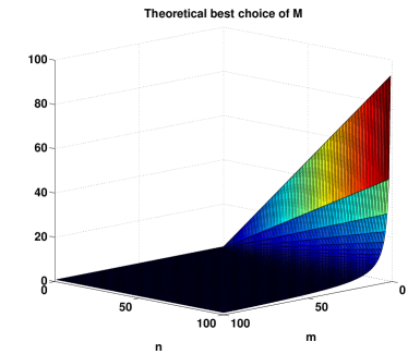
Figure 1: Theoretical maximum relative flop reduction (left) and for which respective choice of $M$ this is obtained (right) for a range of relevant values of $n$ and $m$. In this range a flop reduction of almost up to $30$ times can be achieved. The reduction in the left plot is only plotted for combinations of $n$ and $m$ that will give an improvement.

From the plot it follows that this approach is useful if $m$ is small compared to $n$. In that case, it is beneficial to reformulate the problem as an equivalent control problem with a shorter virtual prediction horizon with more virtual control signals in each virtual sample.

5.2 Decreasing the block-size

This approach is related to what in the Kalman filtering literature is known as sequential processing, where in certain cases the measurement update can be performed sequentially for each one of the measurements in each sample, [10, 7]. The family of formulations achievable with this approach is again parameterized by $M$, which will here decrease the block-size in the resulting sparse numerical linear algebra and make the formulation more sparse as $M$ grows. Since $\tilde{N}=NM$, $\tilde{n}=n$, and $\tilde{m}=m/M$ and the required number of flops for performing a Riccati factorization on the reformulated problem is $f_{2}(M)=N\left(m^{3}/(3M^{2})+4n^{3}M+4m^{2}n/M+6n^{2}m{}\right)$. The theoretical maximum possible gain in flops $f_{2}(1)/f_{2}(M^{*})$ is illustrated in Figure 2 and can be found to be almost as much as a factor of $8$ in the considered problems.

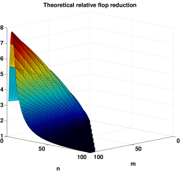
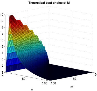
Figure 2: Theoretical maximum relative flop reduction (left) and for which respective choice of $M$ this is obtained (right) for a range of relevant values of $n$ and $m$. In this range a flop reduction of almost up to $8$ times can be achieved. The reduction in the left plot is only plotted for combinations of $n$ and $m$ that will give an improvement.

From the plot it follows that this approach is useful if $n$ is small compared to $m$. In that case, it is beneficial to reformulate the problem with a larger prediction horizon with less control signals in each sample.

Note that, by combining the results from Figures 1 and 2 it can be seen that where the performance gain of one approach is lost, the other one starts to offer a gain. Still, the improvement possible by the presented approaches is only moderate for problems for which $n\approxeq m$, which indicates that the sparsity obtained from the original formulation is a good choice from a performance point of view.

5.3 Combining the approaches

The presented approaches rely on that the original problem’s prediction horizon either is virtually reduced with the cost of having more control signals in each virtual sample, or that the number of control signals is reduced in each virtual sample with the cost of getting a longer virtual prediction horizon. A natural extension is to have a virtual sampling rate over the virtual horizon that is not in sync with the original sampling rate. This can be achieved by combining the two proposed procedures as pointed out in Remark 2 by first increasing the prediction horizon length according to Section 4.2 and then reducing it again according to Section 4.1 with another choice of $M_{k}$ (if the choice of $M_{k}$ is the same in both steps the end result would be the original problem formulation).

Remark 4

The focus in the numerical experiments in this section is serial linear algebra. However, more generally, the proposed reformulations are also interesting for parallel approaches where they for example potentially can be used to optimize the workload distribution.

6 Numerical experiments

In these numerical examples the performance of the proposed strategies is evaluated. The purpose is to investigate how the theoretical improvements in terms of flops in Section 5 are transfered to improvements in terms of computational time. The experiments are performed on an Intel i5-2520M with $8\,$GiB RAM running Windows 7 64-bit. All algorithms, including the Cholesky factorizations, are implemented in m-code in an attempt to make the results relevant for cases where everything is written in the same programming language. If the Cholesky factorization would have been carried out using, e.g., LAPACK calls then the proposed tools could have been used to find other values of $M$ to maximize the overall performance. The reformulations presented in this paper are performed in a preprocessing stage, and the reformulated problems are sent to an implementation of a sparse Riccati KKT system solver. As a comparison, the same problem is also solved, first, using a standard dense formulation using a Cholesky factorization and, second, using the sparse Riccati KKT solver applied to the initial formulation of the problem (block-sizes given by the problem). This experiment basically illustrates the computational complexity of the step direction computation in an optimization routine. To simulate the computations for the search step direction computation in an AS or IP method, the test problems considered are in the form in (1) without any inequality constraints. Note that, the actual choice of examples used in the experiments are irrelevant since the performance of the used linear algebra is only affected by the sizes of problem matrices and not the numbers contained in these. Since the computed direction from the reformulated problem is the same as from the original formulation, apart from minor differences due to differences in the numerics, the number of steps performed by a solver can be expected to be the same independently of which formulation that is used. Since usually the main computational effort in the targeted optimization routines originates from the step direction computation, the overall computational time can be expected to roughly scale as the computational time for the linear algebra which is what is investigated in this section. Furthermore, the KKT solvers used do not at all utilize the structure in the sub-blocks of the reformulated problems, which means that the results shown here can easily be obtained by users without actually making any other changes of their MPC codes rather than the problem formulation as described in earlier sections. It can at least in some cases be expected to be possible to improve these computational times in practice by tailoring parts of the sparse linear algebra, but it would require additional coding.

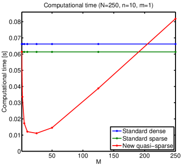
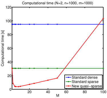
Figure 3: Computational time for the approach in Section 4.1 (left) and the approach in Section 4.2 (right) compared to standard dense and sparse approaches. The respective approaches presented in this work are in the plots denoted “New quasi-sparse”.

From the left plot in Figure 3, it is clear that the performance gain of the approach in Section 4.1 can be significant for the chosen example where $N=250$, $n=10$, and $m=1$. The chosen example is one in which the traditional rule-of-thumb would have suggested that the sparse approach would have been preferable. This is indeed the case, but only with a small margin, and it turns out that the sparse and the dense approaches require $61\,$ms and $66\,$ms, respectively. However, by reformulating the problem using the results presented in Section 4.1 and solving this new formulation using the same sparse Riccati solver, the performance of the sparse approach applied to the reformulated problem is significantly improved and the computational time reduced to $11\,$ms for $M=25$.

From the right plot in Figure 3, it is clear that the performance gain of the approach in Section 4.2 also can be significant for the chosen example where $N=2$, $n=1000$, and $m=1000$. The computational time for the standard sparse method applied to the reformulated problem as proposed in Section 4.2 is $3.8\,$s attained for $M=8$, which should be compared with the standard methods that need $94\,$s and $31\,$s, respectively. Note also, that the chosen example is one in which the traditional rule-of-thumb would have suggested that the dense approach should have been preferable. This is not the case and instead the performance of the sparse one is actually better than the dense one.

7 Conclusions

In this work, two reformulations of MPC problems are presented. The main idea in both reformulations is to trade-off the length of the prediction horizon and the number of control signals in each step along the horizon. This in turn affects the block-size used in the numerical linear algebra and can as such a tool be used to find a formulation of the problem that better utilizes the software libraries and the hardware available on-line. It is shown that these new formulations of the problem can significantly reduce the theoretical number of flops and it is verified in numerical experiments that significant reductions in computational times can be obtained also in practice. More general, the result presented in this work shows that the question to be answered when formulating an MPC problem is not whether a sparse or a dense formulation should be used, but rather how sparse the formulation should be.

Appendix A Definition of stacked matrices

$$\begin{split}\mathsf{x}&=\begin{bmatrix}x_{0}^{T}&x_{1}^{T}&\ldots&x_{N}^{T}\end{bmatrix}^{T},\;\mathsf{u}=\begin{bmatrix}u_{0}^{T}&u_{1}^{T}&\ldots&u_{N-1}^{T}\end{bmatrix}^{T}\\ \mathsf{Q}&=\operatorname{diag}(Q_{0},Q_{1},\ldots,Q_{N}),\;\mathsf{R}=\operatorname{diag}(R_{0},R_{1},\ldots,R_{N-1})\\ S_{x,k}&=\begin{bmatrix}I\\ A\\ A^{2}\\ \vdots\\ A^{k}\end{bmatrix},\;S_{u,k}=\begin{bmatrix}0&0&\ldots&0\\ B&0&\ldots&0\\ AB&B&\ldots&0\\ \vdots&\vdots&\ddots&\vdots\\ A^{k-1}B&A^{k-2}B&\ldots&B\end{bmatrix}\\ \mathsf{A}&=\begin{bmatrix}-I&0&0&\ldots&0\\ A&-I&0&\ldots&0\\ 0&A&-I&\ldots&0\\ 0&\ddots&\ddots&\ddots&0\\ 0&\ldots&0&A&-I\end{bmatrix},\;\mathsf{A}^{-1}=\begin{bmatrix}-I&0&0&\ldots&0\\ -A&-I&0&\ldots&0\\ -A^{2}&-A&-I&\ldots&0\\ \vdots&\ddots&\ddots&\ddots&0\\ -A^{N}&\ldots&0&-A&-I\end{bmatrix},\\ \mathsf{B}&=\begin{bmatrix}0&\ldots&\ldots&0\\ B&0&\ldots&0\\ 0&B&\ldots&0\\ 0&\ddots&\ddots&0\\ 0&\ldots&0&B\end{bmatrix},\\ \mathsf{b}&=\begin{bmatrix}-x^{0\,T}&0&0&\ldots&0\end{bmatrix}^{T}\\ \mathsf{H_{x}}&=\operatorname{diag}\left(H_{x}(0),\ldots,H_{x}(N)){}\right),\;\mathsf{H_{u}}=\operatorname{diag}\left(H_{u}(0),\ldots,H_{u}(N-1)){}\right),\\ \mathsf{h}&=\left[h^{T}(0),\ldots,h^{T}(N){}\right]^{T}\end{split}$$ (16)

Note that, from (16) it follows that $S_{u,N}=-\mathsf{A}^{-1}\mathsf{B}$.

References

- [1] Daniel Axehill. Integer Quadratic Programming for Control and Communication. PhD thesis, Linköping University, 2008.
- [2] Daniel Axehill and Anders Hansson. A mixed integer dual quadratic programming algorithm tailored for MPC. In Proceedings of the 45th IEEE Conference on Decision and Control, pages 5693–5698, Manchester Grand Hyatt, San Diego, USA, December 2006.
- [3] Daniel Axehill and Anders Hansson. A dual gradient projection quadratic programming algorithm tailored for model predictive control. In Proceedings of the 47th IEEE Conference on Decision and Control, pages 3057–3064, Fiesta Americana Grand Coral Beach, Cancun, Mexico, December 2008.
- [4] Daniel Axehill, Anders Hansson, and Lieven Vandenberghe. Relaxations applicable to mixed integer predictive control – comparisons and efficient computations. In Proceedings of the 46th IEEE Conference on Decision and Control, pages 4103–4109, Hilton New Orleans Riverside, New Orleans, USA, December 2007.
- [5] Roscoe A. Bartlett, Lorenz T. Biegler, Johan Backstrom, and Vipin Gopal. Quadratic programming algorithms for large-scale model predictive control. J. Process Contr., 12:775–795, 2002.
- [6] Moritz Diehl, Hans Joachim Ferreau, and Niels Haverbeke. Nonlinear Model Predictive Control, chapter Efficient Numerical Methods for Nonlinear MPC and Moving Horizon Estimation, pages 391–417. Springer Berlin / Heidelberg, 2009.
- [7] Fredrik Gustafsson. Adaptive Filtering and Change Detection. John Wiley & Sons Ltd., 2000.
- [8] Anders Hansson. A primal-dual interior-point method for robust optimal control of linear discrete-time systems. IEEE Trans. Autom. Control, 45(9):1639–1655, September 2000.
- [9] Henrik Jonson. A Newton method for solving non-linear optimal control problems with general constraints. PhD thesis, Linköpings Tekniska Högskola, 1983.
- [10] Thomas Kailath, Ali H. Sayed, and Babak Hassibi. Linear estimation. Prentice Hall, 2000.
- [11] Magnus Åkerblad and Anders Hansson. Efficient solution of second order cone program for model predictive control. Int. J. Contr., 77(1):55–77, 2004.
- [12] I. Nielsen, D. Ankelhed, and D. Axehill. Low-rank modifications of Riccati factorizations with applications to model predictive control. Accepted for publication at CDC 2013, 2013.
- [13] Christopher V. Rao, Stephen J. Wright, and James B. Rawlings. Application of interior-point methods to model predictive control. J. Optimiz. Theory App., 99(3):723–757, December 1998.
- [14] Karl Johan Åström and Björn Wittenmark. Computer controlled systems. Prentice-Hall, 1984.
- [15] Lieven Vandenberghe, Stephen Boyd, and Mehrdad Nouralishahi. Robust linear programming and optimal control. Technical report, Department of Electrical Engineering, University of California Los Angeles, 2002.
- [16] R. Clint Whaley Whaley and Antoine Petitet. Minimizing development and maintenance costs in supporting persistently optimized BLAS. Software: Practice and Experience, 35(2):101–121, February 2005.