Abstract

Let $G$ be a simple graph of order $N$. The normalized Laplacian Estrada index of $G$ is defined as $NEE(G)=\sum_{i=1}^{N}e^{\lambda_{i}}$, where $\lambda_{1},\lambda_{2},\cdots,\lambda_{N}$ are the normalized Laplacian eigenvalues of $G$. In this paper, we give a tight lower bound for $NEE$ of general graphs. We also calculate $NEE$ for a class of treelike fractals, which contain some classical chemical trees as special cases. It is shown that $NEE$ scales linearly with the order of the fractal, in line with a best possible lower bound for connected bipartite graphs.

MSC 2010: 05C50, 15A18, 05C05, 05C90

Keywords: Normalized Laplacian Estrada index, bound, eigenvalue, fractal.

1 Introduction

Let $G$ be a simple undirected graph with vertex set $V(G)=\{v_{1},v_{2}\cdots,v_{N}\}$. Denote by $A=A(G)\in\mathbb{R}^{N\times N}$ the adjacency matrix of $G$, and $\lambda_{1}(A)\geq\lambda_{2}(A)\geq\cdots\geq\lambda_{N}(A)$ the eigenvalues of $A$ in non-increasing order. The Laplacian and normalized Laplacian matrices of $G$ are defined as $L=L(G)=D-A$ and $\mathcal{L}=\mathcal{L}(G)=D^{-1/2}LD^{-1/2}$, respectively, where $D=D(G)$ is a diagonal matrix with $d_{i}$ on the main diagonal being the degree of vertex $v_{i}$, $i=1,\cdots,N$. Here, by convention $d_{i}^{-1}=0$ if $d_{i}=0$. The eigenvalues of $L$ and $\mathcal{L}$ are referred to as the Laplacian and normalized Laplacian eigenvalues of graph $G$, denoted by $\lambda_{1}(L)\geq\lambda_{2}(L)\geq\cdots\geq\lambda_{N}(L)$ and $\lambda_{1}(\mathcal{L})\geq\lambda_{2}(\mathcal{L})\geq\cdots\geq\lambda_{N}(\mathcal{L})$, respectively. Details of the theory of graph eigenvalues can be found in [1, 2].

The Estrada index of a graph $G$ is defined in [3] as

$$EE=EE(G)=\sum_{i=1}^{N}e^{\lambda_{i}(A)},$$

which was first introduced in 2000 as a molecular structure-descriptor by Ernesto Estrada [4]. The Laplacian Estrada index of a graph $G$ is defined in [6] as

$$LEE=LEE(G)=\sum_{i=1}^{N}e^{(\lambda_{i}(L)-2E/N)},$$

where $E$ is the number of edges in $G$. Another essentially equivalent definition for the Laplacian Estrada index is given by $LEE=\sum_{i=1}^{N}e^{\lambda_{i}(L)}$ in [7] independently. Albeit young, the (Laplacian) Estrada index has already found a variety of chemical applications in the degree of folding of long-chain polymeric molecules [5, 8], extended atomic branching [9], and the Shannon entropy descriptor [10]. In addition, noteworthy applications in complex networks are uncovered [11, 12, 13, 14]. Mathematical properties of $EE$ and $LEE$, especially the upper and lower bounds, are investigated in e.g. [15, 16, 17, 18, 19, 20, 21, 22].

Very recently, in full analogy with the (Laplacian) Estrada index, the normalized Laplacian Estrada index of a graph $G$ is introduced in [23] as

$$NEE=NEE(G)=\sum_{i=1}^{N}e^{\lambda_{i}(\mathcal{L})-1}.$$ (1)

Among other things, the following tight bounds for $NEE$ are obtained.

Theorem 1. [23]  If $G$ is a connected graph of order $N$, then

$$NEE\geq(N-1)e^{1/(N-1)}+e^{-1}.$$ (2)

The equality holds if and only if $G=K_{N}$, i.e., a complete graph.

Theorem 2. [23]  Let $G$ be a connected bipartite graph of order $N$ with maximum degree $\Delta$ and minimum degree $\delta$. Then

$$e^{-1}+e+\sqrt{(N-2)^{2}+\frac{2(N-2\Delta)}{\Delta}}\leq NEE\leq e^{-1}+e+(N-3)-\sqrt{\frac{N-2\delta}{\delta}}+e^{\sqrt{\frac{N-2\delta}{\delta}}}.$$ (3)

The equality occurs in both bounds if and only if $G$ is a complete bipartite regular graph.

In this paper, we find a tight lower bound for $NEE$ of a general graph (not necessarily connected) by extending Theorem 1. We also calculate $NEE$ for a class of treelike fractals, which subsume some important chemical trees as special cases, through an explicit recursive relation. We unveil that $NEE$ scales linearly with the order of the fractal, i.e., $NEE\propto N$ for large $N$, in line with the lower bound in Theorem 2.

2 A new lower bound for general graphs

We begin with some basic properties of the normalized Laplacian eigenvalues of a connected graph $G$. In the rest of the paper, to ease notation, we shall use $\lambda_{i}$, $i=1,\cdots,N$ to represent the normalized Laplacian eigenvalues of a graph of order $N$.

Lemma 1. [2]  Let $G$ be a connected graph of order $N\geq 2$. Then

• $\sum_{i=1}^{N}\lambda_{i}=N$.

• $\lambda_{N}=0$ and $\lambda_{i}\in(0,2]$ for every $1\leq i\leq N-1$.

• If $G$ is a bipartite graph, then $\lambda_{1}=2$ and $\lambda_{2}<2$.

Theorem 3.  Let $G$ be a graph of order $N$. If $G$ possesses $c$ connected components, $r$ of which are isolated vertices, then

$$NEE\geq(N-c)e^{\frac{c-r}{N-c}}+ce^{-1}.$$ (4)

The equality holds if and only if $G$ is a union of copies of $K_{s}$, for some fixed $s\geq 2$, and $r$ isolated vertices.

Clearly, we reproduce Theorem 1 when $c=1$ (and $r=0$).

Proof. From Lemma 1 and the fact that the normalized Laplacian eigenvalue for an isolated vertex is zero, we obtain $\lambda_{N}=\cdots=\lambda_{N-c+1}=0$ and $\lambda_{1}+\cdots+\lambda_{N-c}=N-r$. Hence,

$$NEE=e^{-1}\left(c+\sum_{i=1}^{N-c}e^{\lambda_{i}}\right)\geq e^{-1}\left(c+(N-c)e^{\frac{\lambda_{1}+\cdots+\lambda_{N-c}}{N-c}}\right)=ce^{-1}+(N-c)e^{\frac{c-r}{N-c}},$$

where the arithmetic-geometric mean inequality is utilized.

Now suppose $G=(c-r)K_{s}\cup rK_{1}$ for some integers $0\leq r\leq c$ and $s\geq 2$. Then $N=(c-r)s+r=cs-r(s-1)$, and the normalized Laplacian eigenvalues of $G$ can be computed as 0 with multiplicity $c$ and $s/(s-1)$ with multiplicity $(c-r)(s-1)$. Therefore,

$$NEE(G)=ce^{-1}+(c-r)(s-1)e^{\frac{s}{s-1}-1}=ce^{-1}+(N-c)e^{\frac{c-r}{N-c}}.$$

Conversely, suppose that the equality holds in (4). Then from the above application of the arithmetic-geometric mean inequality we know that all the non-zero normalized Laplacian eigenvalues of $G$ must be mutually equal. Suppose that a connected graph $H$ with order $s$ has normalized Laplacian eigenvalues $\lambda>0$ with multiplicity $s-1$ and a single zero eigenvalues. It now suffices to show $H=K_{s}$.

The case of $s=1$ holds trivially. In what follows, we assume $s\geq 2$. We first claim that

$$\mathcal{L}(H)(\mathcal{L}(H)-\lambda I_{s})={\bf 0},$$ (5)

where $I_{s}\in\mathbb{R}^{s\times s}$ is the identity matrix and $\bf 0$ is the zero matrix. Indeed, for any vector $x\in\mathbb{R}^{s}$, we can decompose it as $x=a_{1}D^{1/2}{\bf 1}+\sum_{i=2}^{s}a_{i}x_{i}$, where $a_{i}\in\mathbb{R}$, $\bf 1$ is a column vector with all elements being 1, and $x_{i}$, $i=2,\cdots,s$ are eigenvectors associated with $\lambda$. Thus, the equation (5) follows by the fact that $\mathcal{L}(H)(\mathcal{L}(H)-\lambda I_{s})x=0$ for all $x$.

In the light of (5), all columns of $\mathcal{L}(H)-\lambda I_{s}$ belong to the null space of $\mathcal{L}(H)$. It follows from Lemma 1 that the null space of $\mathcal{L}(H)$ is of dimension one and is spanned by $D^{1/2}\bf 1$. Therefore, each column of $\mathcal{L}(H)-\lambda I_{s}$ is of the form $\alpha D^{1/2}\bf 1$ for some $\alpha\in\mathbb{R}$. Since $H$ is connected, $\alpha\not=0$ and $d_{i}>0$ for all $i$. It follows that any pair of vertices in $H$ must be adjacent in view of the definition of $\mathcal{L}(H)$. This means $H=K_{s}$. $\Box$

3 The normalized Laplacian Estrada index of treelike fractals

In this section, we analytically calculate $NEE$ for a class of treelike fractals through a recursive relation deduced from the self-similar structure of the fractals. It is of great interest to seek $NEE$ (also $LEE$ and $EE$) for specific graphs due to the following two reasons: Firstly, a universal approach for evaluating these structure descriptors of general graphs, especially large-scale graphs, is out of reach so far; and secondly, the known upper and lower bounds (such as (3)) are too far away apart to offer any meaningful guide for a given graph.

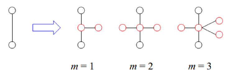
Figure 1: Building blocks of the fractals. The next generation is obtained from current generation through replacing each edge by the stars on the right-hand side of the arrow.

The fractal graphs in question are constructed in an iterative manner [24]. For integers $n\geq 0$ and $m\geq 1$, let $G_{n}(m)$ represent the graph after $n$ iterations (generations). When $n=0$, $G_{0}(m)$ is an edge linking two vertices. In each following iteration $n\geq 1$, $G_{n}(m)$ is built from $G_{n-1}(m)$ by conducting such operations on each existing edges as shown in Fig. 1: subdivide the edge into two edges, connecting to a new vertex; then, generate $m$ new vertices and attach each of them to the middle vertex of the length-2 path. In Fig. 2 are illustrated the first several steps of the iterative construction process corresponding to $m=1$. Clearly, it reduces to two classes of chemical graphs [25]: the $T$ fractal (when $m=1$) and the Peano basin fractal (when $m=2$).

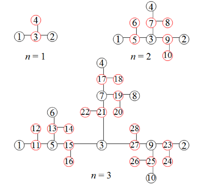
Figure 2: Growth process for a fractal corresponding to $m=1$. The vertex with index 3 is called the inmost vertex since it is in the center of the graph, and those vertices farthest from the inmost vertex are called the outmost vertices (e.g. vertices with indices 1, 2, and 4).

Another intuitive generation approach of the fractal $G_{n}(m)$, which will be used later, highlights the self-similarity. Taking $G_{n}(m)$ with $n=3$ and $m=1$ as an example (see Fig. 2), $G_{n}(m)$ can be obtained by coalescing $m+2$ replicas of $G_{n-1}(m)$ (denoted by $G_{n-1}^{(i)}(m)$, $i=1,\cdots,m+2$) with the $m+2$ outmost vertices in separate duplicates being merged into one single new vertex — the inmost vertex of $G_{n}(m)$ (e.g. the vertex with index 3 in Fig. 2).

Since our results will be stated for any fixed $m$, we often suppress the index $m$ in notations. Some basic properties of $G_{n}=G_{n}(m)$ are easy to derive. For example, the number of vertices and edges are given by $N_{n}=(m+2)^{n}+1$ and $E_{n}=(m+2)^{n}$, respectively. We write $\mathcal{L}_{n}=\mathcal{L}(G_{n})$ as the normalized Laplacian matrix of $G_{n}$. Its eigenvalues are denoted by $\lambda_{1}(n)\geq\lambda_{2}(n)\geq\cdots\geq\lambda_{N_{n}}(n)$. Therefore, the normalized Laplacian Estrada index

$$NEE(G_{n})=\sum_{i=1}^{N_{n}}e^{\lambda_{i}(n)-1}$$ (6)

can be easily derived provided we have all the eigenvalues.

Theorem 4.  All the eigenvalues $\{\lambda_{i}(n)\}_{i=1}^{N_{n}}$, $n\geq 1$ can be obtained by the following recursive relations:

• 0 and 2 are both single eigenvalues for every $n\geq 1$.

• 1 is an eigenvalue with multiplicity $m(m+2)^{n-1}+1$ for $n\geq 1$.

• For $n\geq 1$, all eigenvalues $\lambda(n+1)$ (except 0,1, and 2) at generation $n+1$ are exactly those produced via

  $$\lambda(n+1)=1\pm\sqrt{1-\frac{\lambda(n)}{m+2}}$$ (7)

  by using eigenvalues $\lambda(n)$ (except 0 and 2) at generation $n$.

Proof. We start with checking the completeness of the eigenvalues provided by the rules (i), (ii), and (iii). It is direct to check that the eigenvalues for $G_{1}(m)$ (0, 2, and 1 with multiplicity $m+1$) given by (i) and (ii) are complete. Therefore, all eigenvalues (except 0,1, and 2) for $G_{n}(m)$, $n\geq 2$ are descendants of eigenvalue 1 following (7). Each father eigenvalue produces 2 child eigenvalues in the next generation. Thus, the total number of eigenvalues of $G_{n}(m)$ is found to be

$$2+\sum_{i=0}^{n-1}\left(m(m+2)^{n-1-i}+1\right)2^{i}=(m+2)^{n}+1=N_{n},$$

which implies that all eigenvalues are obtained.

Since $G_{n}$ is connected and bipartite, (i) follows by Lemma 1. It suffices to show (ii) and that each eigenvalue $\lambda_{i}(n+1)$ (except 0,1, and 2) can be derived through (7) by some eigenvalue $\lambda_{i}(n)$. Since $\mathcal{L}_{n}$ is similar to $I_{N_{n}}-D^{-1}(G_{n})A(G_{n})$ thus having the same eigenvalues, we will focus on $I_{N_{n}}-D^{-1}(G_{n})A(G_{n})$ in the sequel and write it as $\mathcal{L}_{n}$ for simplicity.

To derive the recursive relation (7), we resort to the so-called decimation method [26]. Let $\alpha$ denote the set of vertices belonging to $G_{n}$ and $\beta$ the set of vertices created at iteration $n+1$. Assume that $\lambda_{i}(n+1)$ is an eigenvalue of $\mathcal{L}_{n+1}$ and $\lambda_{i}(n+1)\not=0,1,2$. Then the eigenvalue equation for $\mathcal{L}_{n+1}$ can be recast in the following block form

$$\mathcal{L}_{n+1}\left[\begin{array}[]{c}u_{\alpha}\\ u_{\beta}\end{array}\right]=\left[\begin{array}[]{cc}I_{N_{n}}&\mathcal{L}_{\alpha,\beta}\\ \mathcal{L}_{\beta,\alpha}&\mathcal{L}_{\beta,\beta}\end{array}\right]\left[\begin{array}[]{c}u_{\alpha}\\ u_{\beta}\end{array}\right]=\lambda_{i}(n+1)\left[\begin{array}[]{c}u_{\alpha}\\ u_{\beta}\end{array}\right],$$ (8)

where $\mathcal{L}_{\beta,\beta}=I_{E_{n}}\otimes B$ with

$$B=\left[\begin{array}[]{ccccc}1&-\frac{1}{m+2}&-\frac{1}{m+2}&\cdots&-\frac{1}{m+2}\\ -1&1&0&\cdots&0\\ -1&0&1&\cdots&0\\ \vdots&\vdots&\vdots&\ddots&\vdots\\ -1&0&0&\cdots&1\end{array}\right]\in\mathbb{R}^{(m+1)\times(m+1)}.$$

By eliminating $u_{\beta}$ from (8) we arrive at

$$\left(I_{N_{n}}+\mathcal{L}_{\alpha,\beta}(\lambda_{i}(n+1)I_{(m+1)E_{n}}-\mathcal{L}_{\beta,\beta})^{-1}\mathcal{L}_{\beta,\alpha}\right)u_{\alpha}=\lambda_{i}(n+1)u_{\alpha},$$ (9)

provided the concerned matrix is invertible. Let $\mathcal{P}_{n}=I_{N_{n}}+\mathcal{L}_{\alpha,\beta}(\lambda_{i}(n+1)I_{(m+1)E_{n}}-\mathcal{L}_{\beta,\beta})^{-1}\mathcal{L}_{\beta,\alpha}$ and $\mathcal{Q}_{n}=(x+y)I_{N_{n}}-y\mathcal{L}_{n}$, with

$$x=\frac{\lambda_{i}(n+1)-1}{(m+2)(\lambda_{i}(n+1)-2)\lambda_{i}(n+1)+2}+1=y+1.$$ (10)

It is not difficult to see that $\mathcal{P}_{n}=\mathcal{Q}_{n}$.

Indeed,

$$(\lambda_{i}(n+1)I_{(m+1)E_{n}}-\mathcal{L}_{\beta,\beta})^{-1} = I_{E_{n}}\otimes(\lambda_{i}(n+1)I_{m+1}-B)^{-1}$$

$$= I_{E_{n}}\otimes\frac{\mathrm{adj}((\lambda_{i}(n+1)I_{m+1}-B))}{\det((\lambda_{i}(n+1)I_{m+1}-B)},$$

where $\mathrm{adj}(\cdot)$ means the adjugate matrix. Let $z$ be the element on the first row and the first column of $(\lambda_{i}(n+1)I_{m+1}-B)^{-1}$. We have

$$z=\frac{(\lambda_{i}(n+1)-1)^{m}}{\det((\lambda_{i}(n+1)I_{m+1}-B)}=\frac{(m+2)(\lambda_{i}(n+1)-1)}{2+(m+2)\lambda_{i}(n+1)(\lambda_{i}(n+1)-2)},$$

which is well-defined since $\lambda_{i}(n+1)\not=0,2$. With these preparations, it is easy to make an entry-wise comparison between $\mathcal{P}_{n}$ and $\mathcal{Q}_{n}$. Clearly, $(\mathcal{Q}_{n})_{i,i}=x=1+d_{i}(-1/d_{i})z(-1/(m+2))=(\mathcal{P}_{n})_{i,i}$; for $i\not=j$, if $i$ and $j$ are not adjacent, $(\mathcal{Q}_{n})_{i,j}=(\mathcal{P}_{n})_{i,j}=0$, while if $i$ and $j$ are adjacent, $(\mathcal{Q}_{n})_{i,j}=-y(-1/d_{i})=(-1/d_{i})z(-1/(m+2))=(\mathcal{P}_{n})_{i,j}$. Hence, we conclude $\mathcal{P}_{n}=\mathcal{Q}_{n}$.

Inserting the equality $\mathcal{P}_{n}=\mathcal{Q}_{n}$ into (9) we get

$$\mathcal{L}_{n}u_{\alpha}=\left(\frac{x+y-\lambda_{i}(n+1)}{y}\right)u_{\alpha},$$

where $y\not=0$ since $\lambda_{i}(n+1)\not=1$. This indicates that $\lambda_{i}(n)=(x+y-\lambda_{i}(n+1))/y$, where $\lambda_{i}(n)$ is an eigenvalue of $\mathcal{L}_{n}$ associated with the eigenvector $u_{\alpha}$. Combining this with (10) yields a quadratic equation, whose solution gives the formula (7) as desired.

It remains to show (ii). Let $M_{n}(\lambda)$ represent the multiplicity of eigenvalue $\lambda$ of $\mathcal{L}_{n}$. We have

$$M_{n}(\lambda=1)=N_{n}-\mathrm{rank}(\mathcal{L}_{n}-I_{N_{n}}).$$

The problem of determining multiplicity is reduced to evaluating $\mathrm{rank}(\mathcal{L}_{n}-I_{N_{n}})$. (ii) follows by showing that

$$\mathrm{rank}(\mathcal{L}_{n}-I_{N_{n}})=2(m+2)^{n-1}$$ (11)

for each $n\geq 1$.

To show (11) we use the method of induction. For $n=1$, we have

$$\mathcal{L}_{1}-I_{N_{1}}=\left[\begin{array}[]{cccc}0&-\frac{1}{m+2}&\cdots&-\frac{1}{m+2}\\ -1&0&\cdots&0\\ \vdots&\vdots&\ddots&\vdots\\ -1&0&\cdots&0\end{array}\right]\in\mathbb{R}^{(m+3)\times(m+3)}.$$

Thus, $\mathrm{rank}(\mathcal{L}_{1}-I_{N_{1}})=2$. For $n=2$, we have

$$\mathcal{L}_{2}-I_{N_{2}}=\left[\vbox{\hbox{\kern-1.15198pt\raise 0.0pt\hbox{\kern 79.42015pt}\kern 0.0pt\vbox{}\kern-1.15198pt}}\right],$$

where $F\in\mathbb{R}^{(m+2)\times(m+2)}$ is the matrix $\mathcal{L}_{1}-I_{N_{1}}$ deleting the last column and the last row. Accordingly, $\mathrm{rank}(\mathcal{L}_{2}-I_{N_{2}})=2(m+2)$. For $n\geq 2$, we have

$$\mathcal{L}_{n+1}-I_{N_{n+1}}=\left[\vbox{\hbox{\kern-1.15198pt\raise 0.0pt\hbox{\kern 82.78146pt}\kern 0.0pt\vbox{}\kern-1.15198pt}}\right],$$

where $F_{n}+I_{(m+2)^{n}}=\mathcal{L}(G_{n}\backslash\{\mathrm{an}\ \mathrm{outmost}\ \mathrm{vertex}\})$. Moreover, $F_{n}$ can be iteratively expressed as

$$F_{n}=\left[\begin{array}[]{ccccc}F_{n-1}&0&\cdots&0&w_{1}\\ 0&F_{n-1}&\cdots&0&w_{2}\\ \vdots&\vdots&\ddots&\vdots&\vdots\\ 0&0&\cdots&F_{n-1}&w_{m+1}\\ w_{1}^{T}&w_{2}^{T}&\cdots&w_{m+1}^{T}&F_{n-1}\end{array}\right],$$

where each $w_{i}\in\mathbb{R}^{(m+2)^{n-1}\times(m+2)^{n-1}}$ is a matrix containing only one non-zero element $-1/(m+2)$ describing the edge linking the inmost vertex in $G_{n}$ to one vertex in the replica $G_{n-1}^{(i)}$. For any vertex $u$ in $G_{n}$ that is adjacent to the inmost vertex of $G_{n}$, it has a neighbor $v$ with degree one. Hence, there is only one non-zero element for row $v$ and for column $v$, respectively, that is, $(F_{n})_{v,u}=-1$ and $(F_{n})_{u,v}=-1/(m+2)$. By using some basic operations for the matrix, we can eliminate all non-zero elements at the last row and the last column of $F_{n}$. Thus, $\mathrm{rank}(\mathcal{L}_{n+1}-I_{N_{n+1}})=(m+2)\cdot\mathrm{rank}(F_{n})=(m+2)\cdot\mathrm{rank}(\mathcal{L}_{n}-I_{N_{n}})$. This yields (11), and finally concludes the proof. $\Box$

Remark 1. We mention that although the eigenvalues of a related matrix of $G_{n}(m)$ have been computed in [27] by a semi-analytical method, the normalized Laplacian eigenvalues cannot be derived directly from results therein.

With Theorem 4 at hand, the normalized Laplacian Estrada index can be easily evaluated through (6). Note that $G_{n}(m)$ is a connected bipartite graph with maximum degree $\Delta=m+2$ and minimum degree $\delta=1$. In Fig. 3, we display $NEE(G_{n}(m))$ for $n=1,\cdots,7$, $m=1,\cdots,5$ together with the obtained bounds in Theorem 2. The results gathered in Fig. 3 allow us to draw several interesting comments. First, as expected from Theorem 2, all values of $NEE(G_{n}(m))$ lie between the upper and lower bounds. Second, the lower bounds for different values of $\Delta$ are collapsed together and they scale with the order of the graph as $NEE\propto N$, which can be derived from (3). Similarly, the upper bound scales with $N$ as $NEE\propto e^{\sqrt{N}}$. Third, $NEE(G_{n}(m))$ also scales linearly with the order of the fractal, i.e., $NEE(G_{n}(m))\propto N_{n}$, in parallel with the lower bound.

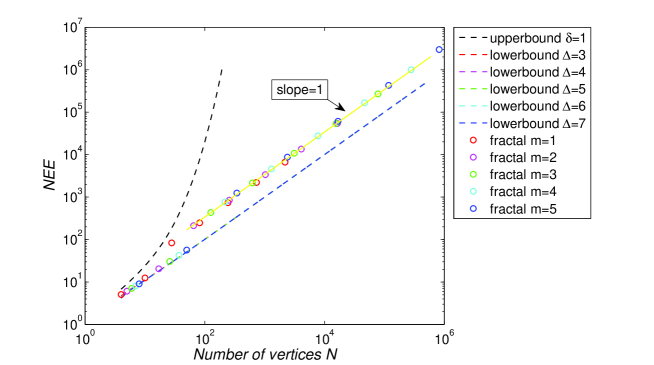
Figure 3: The normalized Laplacian Estrada index $NEE$ versus the number of vertices $N$ in log-log scale. Circles represent $NEE(G_{n}(m))$ for $n=1,\cdots,7$, $m=1,\cdots,5$; dashed lines represent the bounds given by (3).

References

- [1] D. M. Cvetković, M. Doob, H. Sachs, Spectra of Graphs: Theory and Application. Johann Ambrosius Bart Verlag, Heidelberg, 1995
- [2] F. Chung, Spectral Graph Theory. Amer. Math. Soc., Providence, 1997
- [3] J. A. de la Peña, I. Gutman, J. Rada, Estimating the Estrada index. Linear Algebra Appl., 427(2007) 70–76
- [4] E. Estrada, Characterization of 3D molecular structure. Chem. Phys. Lett., 319(2000) 713–718
- [5] E. Estrada, Characterization of the folding degree of proteins. Bioinformatics, 18(2002) 697–704
- [6] J. Li, W. C. Shiu, A. Chang, On the Laplacian Estrada index of a graph. Appl. Anal. Discrete Math., 3(2009) 147–156
- [7] G. H. Fath-Tabar, A. R. Ashrafi, I. Gutman, Note on Estrada and -Estrada indices of graphs. Bull. Acad. Serbe Sci. Arts Cl. Sci. Math., 139(2009) 1–16
- [8] E. Estrada, Characterization of the folding degree of proteins. Bioinformatics, 18(2002) 697–704
- [9] E. Estrada, J. A. Rodríguez-Velázquez, M. Randić, Atomic branching in molecules. Int. J. Quantum Chem., 106(2006) 823–832
- [10] R. Carbó-Dorca, Smooth function topological structure descriptors based on graph-spectra. J. Math. Chem., 44(2008) 373–378
- [11] E. Estrada, J. A. Rodríguez-Velázquez, Subgraph centrality in complex networks. Phys. Rev. E, 71(2005) 056103
- [12] E. Estrada, J. A. Rodríguez-Velázquez, Spectral measures of bipartivity in complex networks. Phys. Rev. E, 72(2005) 046105
- [13] Y. Shang, Perturbation results for the Estrada index in weighted networks. J. Phys. A: Math. Theor., 44(2011) 075003
- [14] Y. Shang, Local natural connectivity in complex networks. Chin. Phys. Lett., 28(2011) 068903
- [15] J. Li, W. C. Shiu, W. H. Chan, Note on the Laplacian Estrada index of a graph. MATCH Commun. Math. Comput. Chem., 66(2011) 777–784
- [16] B. X. Zhu, On the Laplacian Estrada index of graphs. MATCH Commun. Math. Comput. Chem., 66(2011) 769–776
- [17] I. Gutman, Lower bounds for Estrada index. Publ. Inst. Math. Beograd, 83(2008) 1–7
- [18] B. Zhou, On Estrada index. MATCH Commun. Math. Comput. Chem., 60(2008) 485–492
- [19] A. Khosravanirad, A lower bound for Laplacian Estrada index of a graph. MATCH Commun. Math. Comput. Chem., 70(2013) 175–180
- [20] H. Bamdad, F. Ashraf, I. Gutman, Lower bounds for Estrada index and Laplacian Estrada index. Appl. Math. Lett., 23(2010) 739–742
- [21] Y. Shang, Lower bounds for the Estrada index of graphs. Electron. J. Linear Algebra, 23(2012) 664–668
- [22] Y. Shang, Lower bounds for the Estrada index using mixing time and Laplacian spectrum. Rocky Mountain J. Math., 43(2013) in press
- [23] J. Li, J.-M. Guo, W. C. Shiu, The normalized Laplacian Estrada index of a graph. Filomat, in press
- [24] Y. Lin, B. Wu, Z. Zhang, Determining mean first-passage time on a class of treelike regular fractals. Phys. Rev. E, 82(2010) 031140
- [25] N. Trinajstić, Chemical Graph Theory. CRC Press, Boca Raton, 1992
- [26] N. Lal, M. L. Lapidus, The decimation method for Laplacians on fractals: spectra and complex dynamics. in: Fractal Geometry and Dynamical Systems in Pure and Applied Mathematics II: Fractals in Applied Mathematics (D. Carfi, M. L. Lapidus, E. P. J. Pearse, and M. van Frankenhuijsen, eds.), Amer. Math. Soc., Providence, 2013
- [27] Z. Zhang, B. Wu, G. Chen, Complete spectrum of the stochastic master equation for random walks on treelike fractals. EPL, 96(2011) 40009