Coherent control of optical injection of spin and currents in topological insulators

Abstract

Topological insulators have surface states with a remarkable helical spin structure, with promising prospects for applications in spintronics. Strategies for generating spin polarized currents, such as the use of magnetic contacts and photoinjection, have been the focus of extensive research. While several optical methods for injecting currents have been explored, they have all focused on one-photon absorption.

Here we consider the use of both a fundamental optical field and its second harmonic, which allows the injection of spin polarized carriers and current by a nonlinear process involving quantum interference between one- and two-photon absorption. General expressions are derived for the injection rates in a generic two-band system, including those for one- and two-photon absorption processes as well as their interference. Results are given for carrier, spin density and current injection rates on the surface of topological insulators, for both linearly and circularly polarized light. We identify the conditions that would be necessary for experimentally verifying these predictions.

I Introduction

Three-dimensional topological insulators are fascinating materials, with a band gap in the bulk and protected midgap states on their surfaces hasan10 ; qi11 . The surface electronic bands are described by a single Dirac cone with a helical spin structure, which is the equivalent of a dominant Rashba spin-orbit coupling term in the Hamiltonian. This property leads to a number of interesting features, including non-magnetic scattering, the magnetoelectric effect qi08 ; essin09 , and the formation of Majorana fermions in the proximity of superconductors fu08 . Due to the effective spin-orbit coupling, the spin and current of the surface states are closely related raghu10 , providing an exciting opportunity for technological applications using spin polarized currents. There have already been several studies using the proximity of a magnetic metal for injecting spin polarization and current butch12 ; modak12 ; semenov12 ; mahfouzi12 .

Another fruitful approach for manipulating currents in materials involves optical excitation. The optical properties of topological insulator surface states are very interesting themselves, with features such as the injected current depending explicitly on the Berry phase tse10 ; hosur11 . The injection of spin and current by one photon absorption processes has been studied in different circumstances hosur11 ; misawa11 ; mciver12nn . In order to break the rotational symmetry stemming from the Dirac cone - a necessary step for generating a current - the use of an in-plane magnetic field, the application of strain, and an oblique angle of incidence have all been considered. Corrections due to snowflake warping have been included; even a surprisingly relevant contribution from the Zeeman coupling of the light field has been identified refael13 . Nonlinear effects due to the second harmonic have also been considered hsieh11a ; hsieh11b ; mciver12prb ; sobota12 , especially in the treatment of pulses. However the focus of even these studies has been on one photon absorption processes.

One of the most interesting techniques for optical injection is coherent control, an example of which involves tuning the interference of one and two photon absorption processes to achieve a target response. This has been employed for injecting carriers, spin polarization, currents, and spin currents in semiconductors rioux12 ; kiran11 , and currents in graphene norris10 ; rioux11 ; kiran12 . It has even been proposed that it could be used to inject a macroscopic Berry curvature in semiconductor quantum wells virk11 . Here we present predictions of the optical injection of carrier density, spin polarization, charge current, and spin current at the surface of a topological insulator. In order to identify the fundamental properties of coherent control in topological insulators, we use a Hamiltonian with a perfectly symmetric Dirac cone, and restrict the analysis to light at normal incidence. This also helps to contrast the results of coherent control with those obtained by other means. We keep a $\sigma_{z}$ mass term in the Hamiltonian in order to analyze the dependence on the Berry phase, which has interesting effects on the injection rates.

In Sec. II we present the calculation of optical injection rates for an arbitrary quantity using Fermi’s golden rule, considering one and two photons absorption processes as well as their interference. In Sec. III we provide general expressions for the injection rates of a generic two-band system, especially for carrier density, spin density, charge current and spin current operators. Since two-band models can be used, as a first approximation, to compute optical properties of a large number of materials, the expressions derived there should be of use even beyond their application to topological insulators. In Sec. IV we apply the results of Sec. III to topological insulators. In Sec. V we present the results for linearly and circularly polarized light, referring to the Appendices A and B for details. In Sec. VI we end with a discussion of interesting features in our results and the possibilities for their experimental verification, including estimates for the expected experimental results. Since the experimental techniques required to confirm our results are well established, we can expect that such experiments will help advance the understanding and applications of topological insulators.

II Response to light fields

There are several methods for computing the response of a system to external perturbations; one of the simplest and most standard methods is Fermi’s golden rule. It is especially suitable for coherent control calculations because it makes evident all the contributions stemming from one- and two-photon processes and their interference. This is a feature not shared by the Kubo formalism, for instance.

The calculation for the injection rates of operators using Fermi’s golden rule has been already well explained in previous studies rioux12 . However, it has been typically assumed that the fundamental photon energy is below the bandgap, as is the case for most studies of semiconductors. Since we will deal with systems that are gapless, there will be an additional interference term. And in order to make the notation clear we will present the main steps of the full calculation.

The full Hamiltonian in the presence of the external perturbation $V_{ext}\left(t\right)$ is $H\left(t\right)=H_{0}+V_{ext}\left(t\right)$, where $H_{0}$ is the Hamiltonian without the perturbation. The wavefunction in the presence of the external perturbation can have a contribution from an excitation of a valence $v$ band electron to a conduction $c$ band

$$\begin{array}[]{rl}\left|\Psi\left(t\right)\right\rangle=&c_{0}\left|0\right\rangle+c_{cv,\bm{k}}\left(t\right)\left|cv,\bm{k}\right\rangle+\dots,\\ \rho_{cv,\bm{k}}=&\left|c_{cv,\bm{k}}\right|^{2},\end{array}$$ (1)

where $\left|0\right\rangle$ is the groundstate of $H_{0}$ with filled valence bands; $\left|cv,\bm{k}\right\rangle=a_{c,\bm{k}}^{\dagger}a_{v,\bm{k}}\left|0\right\rangle$ is the state with an electron-hole pair, with $a_{c,\bm{k}}^{\dagger}$ denoting the electron creation operator, and

$$\begin{array}[]{rl}c_{cv,\bm{k}}\left(t\right)=&\int_{-\infty}^{t}\frac{dt_{1}}{i\hbar}e^{-i\omega_{cv}t}\vartheta_{cv,\bm{k}}^{\left(1\right)}\left(t_{1}\right)\\ &+\int_{-\infty}^{t}\frac{dt_{1}}{i\hbar}\int_{-\infty}^{t_{1}}\frac{dt_{2}}{i\hbar}e^{-i\omega_{cv}t}\vartheta_{cv,\bm{k}}^{\left(2\right)}\left(t_{1},t_{2}\right),\end{array}$$ (2)

where $\omega_{cv}=\omega_{c}-\omega_{v}$; here $\vartheta_{cv,\bm{k}}^{\left(1\right)}\left(t_{1}\right)=\left\langle cv,\bm{k}\right|V_{ext}\left(t_{1}\right)\left|0\right\rangle$ and $\vartheta_{cv,\bm{k}}^{\left(2\right)}\left(t_{1},t_{2}\right)=\left\langle cv,\bm{k}\right|V_{ext}\left(t_{1}\right)V_{ext}\left(t_{2}\right)\left|0\right\rangle$. This allows us to compute the injection rate for the density $\left\langle M\right\rangle$ of a quantity associated with a single-particle operator ${\cal M}=\sum_{\bm{k}}a_{\alpha,\bm{k}}^{\dagger}M_{\alpha\beta,\bm{k}}a_{\beta,\bm{k}}$, where $\alpha$ and $\beta$ are band indices. The expression for $\left\langle\dot{M}\right\rangle$ is

$$\frac{d}{dt}\left\langle M\right\rangle=\frac{1}{L^{D}}\sum_{cv,c^{\prime}v^{\prime},\bm{k}}\left(M_{c^{\prime}c,\bm{k}}\delta_{v^{\prime}v}-M_{v^{\prime}v,\bm{k}}\delta_{c^{\prime}c}\right)\frac{d}{dt}\left(c_{c^{\prime}v^{\prime},\bm{k}}^{\ast}c_{cv,\bm{k}}\right),$$ (3)

where $L$ is the unidimensional length and $D$ is the spatial dimension of the system.

Specifying the perturbation to be an incident laser field, using the minimal coupling Hamiltonian we have

$$\begin{array}[]{rl}\vartheta_{cv,\bm{k}}\left(t_{1}\right)=&-\frac{e}{c}\bm{v}_{cv,\bm{k}}\cdot\bm{A}\left(t_{1}\right)e^{i\omega_{cv}t_{1}},\\ \vartheta_{cv,\bm{k}}^{\left(2\right)}\left(t_{1},t_{2}\right)=&\frac{e^{2}}{c^{2}}\underset{c^{\prime}}{\sum}\bm{v}_{cc^{\prime}}\cdot\bm{A}\left(t_{1}\right)e^{i\omega_{cc^{\prime}}t_{1}}\bm{v}_{c^{\prime}v}\cdot\bm{A}\left(t_{2}\right)e^{i\omega_{c^{\prime}v}t_{2}}\\ &-\frac{e^{2}}{c^{2}}\underset{v^{\prime}}{\sum}\bm{v}_{v^{\prime}v}\cdot\bm{A}\left(t_{1}\right)e^{i\omega_{v^{\prime}v}t_{1}}\bm{v}_{cv^{\prime}}\cdot\bm{A}\left(t_{2}\right)e^{i\omega_{cv^{\prime}}t_{2}},\end{array}$$ (4)

where $e=-\left|e\right|$ is the charge of the electron, $\bm{v}$ is the velocity operator, and the vector potential is

$$\bm{A}\left(t\right)=\sum_{\omega_{\alpha}}\bm{A}\left(\omega_{\alpha}\right)e^{-i\left(\omega_{\alpha}+i\epsilon\right)t},$$ (5)

with $\omega_{\alpha}=\pm\omega,\pm 2\omega$; here $\epsilon\to 0^{+}$ describes the turning on of the field from $t=-\infty$.

From Eq. (2) we can write $c_{cv,\bm{k}}\left(t\right)$ as

$$c_{cv,\bm{k}}\left(t\right)=\sum_{n=1}^{4}K_{cv,\bm{k}}^{\left(n\right)}\left(\omega\right)\frac{e^{-i\left(n\omega+i\epsilon\right)t}}{n\omega-\omega_{cv}+i\epsilon},$$ (6)

where

$$\begin{array}[]{rl}K_{cv,\bm{k}}^{\left(1\right)}\left(\omega\right)=&-\frac{e}{\hbar c}\bm{v}_{cv,\bm{k}}\cdot\bm{A}\left(\omega\right)+\\ &+\frac{e^{2}}{\hbar^{2}c^{2}}\underset{v^{\prime}c^{\prime}}{\sum}\frac{\bm{v}_{cc^{\prime}}\cdot\bm{A}\left(-\omega\right)\bm{v}_{c^{\prime}v}\cdot\bm{A}\left(2\omega\right)}{2\omega-\omega_{c^{\prime}v}+i\epsilon}-\frac{\bm{v}_{v^{\prime}v}\cdot\bm{A}\left(-\omega\right)\bm{v}_{cv^{\prime}}\cdot\bm{A}\left(2\omega\right)}{2\omega-\omega_{cv^{\prime}}+i\epsilon}\\ &+\frac{e^{2}}{\hbar^{2}c^{2}}\underset{v^{\prime}c^{\prime}}{\sum}\frac{\bm{v}_{cc^{\prime}}\cdot\bm{A}\left(2\omega\right)\bm{v}_{c^{\prime}v}\cdot\bm{A}\left(-\omega\right)}{-\omega-\omega_{c^{\prime}v}+i\epsilon}-\frac{\bm{v}_{v^{\prime}v}\cdot\bm{A}\left(2\omega\right)\bm{v}_{cv^{\prime}}\cdot\bm{A}\left(-\omega\right)}{-\omega-\omega_{cv^{\prime}}+i\epsilon},\end{array}$$ (7)

and

$$\begin{array}[]{rl}K_{cv,\bm{k}}^{\left(2\right)}\left(\omega\right)=&-\frac{e}{\hbar c}\bm{v}_{cv,\bm{k}}\cdot\bm{A}\left(2\omega\right)+\\ &+\frac{e^{2}}{\hbar^{2}c^{2}}\underset{v^{\prime}c^{\prime}}{\sum}\frac{\bm{v}_{cc^{\prime}}\cdot\bm{A}\left(\omega\right)\bm{v}_{c^{\prime}v}\cdot\bm{A}\left(\omega\right)}{\omega-\omega_{c^{\prime}v}+i\epsilon}-\frac{\bm{v}_{v^{\prime}v}\cdot\bm{A}\left(\omega\right)\bm{v}_{cv^{\prime}}\cdot\bm{A}\left(\omega\right)}{\omega-\omega_{cv^{\prime}}+i\epsilon},\end{array}$$ (8)

with similar expressions for $K_{cv,\bm{k}}^{\left(3\right)}$ and $K_{cv,\bm{k}}^{\left(4\right)}$; the first only has terms with products of field amplitudes $A\left(\pm\omega\right)A\left(\pm 2\omega\right)$, and the second only has terms with products $A\left(\pm 2\omega\right)A\left(\pm 2\omega\right)$. Then we have

$$\begin{array}[]{rl}\frac{d}{dt}\left(c_{c^{\prime}v^{\prime},\bm{k}}^{\ast}c_{cv,\bm{k}}\right)_{t=0}=&\pi\underset{n}{\sum}K_{c^{\prime}v^{\prime},\bm{k}}^{\left(n\right)\ast}\left(\omega\right)K_{cv,\bm{k}}^{\left(n\right)}\left(\omega\right)\\ &\cdot\left[\delta\left(n\omega-\omega_{cv,\bm{k}}\right)+\delta\left(n\omega-\omega_{c^{\prime}v^{\prime},\bm{k}}\right)\right].\end{array}$$ (9)

We assume that the amplitude $A\left(\pm 2\omega\right)$ of the second harmonic field is much smaller that the amplitude $A\left(\pm\omega\right)$ of the fundamental field. Since two-photon processes are much weaker than one-photon processes, two-photon processes involving the second harmonic are then neglected, and only $K_{cv,\bm{k}}^{\left(1\right)}\left(\omega\right)$ and $K_{cv,\bm{k}}^{\left(2\right)}\left(\omega\right)$ remain. Since $K_{cv,\bm{k}}^{\left(3\right)}\left(\omega\right)$ and $K_{cv,\bm{k}}^{\left(4\right)}\left(\omega\right)$ do not have linear terms in the field amplitude they do not support any interference process, but only two-photon absorption.

Since all the $K_{cv,\bm{k}}^{\left(n\right)}\left(\omega\right)$ are multiplied by a $\delta$ function in Eq. (9), we can write

$$\begin{array}[]{rl}K_{cv,\bm{k}}^{\left(1\right)}\left(\omega\right)=&\frac{ie}{\hbar\omega}v_{cv,\bm{k}}^{b}E^{b}\left(\omega\right)\\ &-{\cal W}_{cv,\bm{k}}^{bc}\left(2\omega,-\omega\right)E^{b}\left(-\omega\right)E^{c}\left(2\omega\right),\\ K_{cv,\bm{k}}^{\left(2\right)}\left(\omega\right)=&\frac{ie}{2\hbar\omega}v_{cv,\bm{k}}^{b}E^{b}\left(2\omega\right)\\ &+{\cal W}_{cv,\bm{k}}^{bc}\left(\omega,\omega\right)E^{b}\left(\omega\right)E^{c}\left(\omega\right),\end{array}$$ (10)

where

$$\begin{array}[]{rl}\Omega_{cv,\bm{k}}^{bc}\left(\omega_{\alpha}\right)=&\frac{-e^{2}}{\hbar^{2}\omega^{2}}\underset{n}{\sum}\frac{v_{cn}^{b}v_{nv}^{c}}{\omega_{\alpha}-\omega_{nv}},\\ {\cal W}_{cv,\bm{k}}^{bc}\left(\omega_{\alpha},\omega_{\beta}\right)=&\Omega_{cv,\bm{k}}^{bc}\left(\omega_{\alpha}\right)+\Omega_{cv,\bm{k}}^{cb}\left(\omega_{\beta}\right),\end{array}$$ (11)

and $\bm{E}\left(t\right)=-c^{-1}\partial_{t}\bm{A}\left(t\right)$ was used, so $\bm{A}\left(n\omega\right)=-ic\left(n\omega\right)^{-1}\bm{E}\left(n\omega\right)$. The injection rate for an operator ${\cal M}$ can then be decomposed into contributions from one and two photons absorption processes with an additional interference term $\left\langle\dot{M}\right\rangle=\left\langle\dot{M}_{1}\right\rangle+\left\langle\dot{M}_{2}\right\rangle+\left\langle\dot{M}_{i}\right\rangle$ where

$$\begin{array}[]{rl}\left\langle\dot{M}_{1}\right\rangle=&\underset{n=1,2}{\sum}\Lambda_{1}^{bc}\left(n\omega\right)E^{b}\left(-n\omega\right)E^{c}\left(n\omega\right),\\ \left\langle\dot{M}_{2}\right\rangle=&\Lambda_{2}^{bcde}\left(\omega\right)E^{b}\left(-\omega\right)E^{c}\left(-\omega\right)E^{d}\left(\omega\right)E^{e}\left(\omega\right),\\ \left\langle\dot{M}_{i}\right\rangle=&\underset{n=1,2}{\sum}\Lambda_{i\left(n\right)}^{bcd}\left(\omega\right)E^{b}\left(-\omega\right)E^{c}\left(-\omega\right)E^{d}\left(2\omega\right)+cc,\end{array}$$ (12)

with

$$\begin{array}[]{rl}\Lambda_{1}^{bc}\left(n\omega\right)=&\frac{\pi}{L^{D}}\underset{cv,c^{\prime}v^{\prime},\bm{k}}{\sum}\left(M_{c^{\prime}c,\bm{k}}\delta_{v^{\prime}v}-M_{v^{\prime}v,\bm{k}}\delta_{c^{\prime}c}\right)\Gamma_{1,c^{\prime}v^{\prime},cv}^{bc}\left(\bm{k},\omega\right)\left[\delta\left(n\omega-\omega_{cv,\bm{k}}\right)+\delta\left(n\omega-\omega_{c^{\prime}v^{\prime},\bm{k}}\right)\right],\\ \Lambda_{2}^{bcde}\left(\omega\right)=&\frac{\pi}{L^{D}}\underset{cv,c^{\prime}v^{\prime},\bm{k}}{\sum}\left(M_{c^{\prime}c,\bm{k}}\delta_{v^{\prime}v}-M_{v^{\prime}v,\bm{k}}\delta_{c^{\prime}c}\right)\Gamma_{2,c^{\prime}v^{\prime},cv}^{bcde}\left(\bm{k},\omega\right)\left[\delta\left(2\omega-\omega_{cv,\bm{k}}\right)+\delta\left(2\omega-\omega_{c^{\prime}v^{\prime},\bm{k}}\right)\right],\\ \Lambda_{i\left(n\right)}^{bcd}\left(\omega\right)=&\frac{\pi}{L^{D}}\underset{cv,c^{\prime}v^{\prime},\bm{k}}{\sum}\left(M_{c^{\prime}c,\bm{k}}\delta_{v^{\prime}v}-M_{v^{\prime}v,\bm{k}}\delta_{c^{\prime}c}\right)\Gamma_{i\left(n\right),c^{\prime}v^{\prime},cv}^{bcd}\left(\bm{k},\omega\right)\left[\delta\left(n\omega-\omega_{cv,\bm{k}}\right)+\delta\left(n\omega-\omega_{c^{\prime}v^{\prime},\bm{k}}\right)\right],\end{array}$$ (13)

and

$$\begin{array}[]{rl}\Gamma_{1,c^{\prime}v^{\prime},cv}^{bc}\left(\bm{k},\omega\right)=&\frac{e^{2}}{\hbar^{2}\omega^{2}}v_{v^{\prime}c^{\prime}}^{b}v_{cv}^{c},\\ \Gamma_{2,c^{\prime}v^{\prime},cv}^{bcde}\left(\bm{k},\omega\right)=&{\cal W}_{c^{\prime}v^{\prime},\bm{k}}^{bc}\left(\omega,\omega\right)^{\ast}{\cal W}_{cv,\bm{k}}^{de}\left(\omega,\omega\right),\\ \Gamma_{i\left(1\right),c^{\prime}v^{\prime},cv}^{bcd}\left(\bm{k},\omega\right)=&\frac{ie}{\hbar\omega}v_{v^{\prime}c^{\prime}}^{b}{\cal W}_{cv,\bm{k}}^{cd}\left(2\omega,-\omega\right),\\ \Gamma_{i\left(2\right),c^{\prime}v^{\prime},cv}^{bcd}\left(\bm{k},\omega\right)=&\frac{ie}{2\hbar\omega}{\cal W}_{cv,\bm{k}}^{bc}\left(\omega,\omega\right)^{\ast}v_{c^{\prime}v^{\prime}}^{d}.\end{array}$$ (14)

The $\Lambda_{1}^{bc}\left(\omega\right)$ and $\Lambda_{i\left(1\right)}^{bcd}\left(\omega\right)$ terms have usually been ignored in the literature, since they vanish for systems with a gap where the first harmonic falls below the bandgap. The two interference processes are shown in Fig. 1. The quantities for which the injection rates will be computed are the densities associated with the carriers $\left\langle n\right\rangle$, spin $\left\langle\bm{S}\right\rangle$, charge current $\left\langle\bm{J}_{c}\right\rangle$, and spin current $\left\langle\bm{J}_{S}\right\rangle$. We denote the response coefficients associated with the quantities $\left\langle\dot{n}\right\rangle$, $\left\langle\dot{\bm{S}}\right\rangle$, $\left\langle\dot{\bm{J}}_{c}\right\rangle$, $\left\langle\dot{\bm{J}}_{S}\right\rangle$ respectively by $\xi$, $\zeta$, $\eta$, $\mu$.

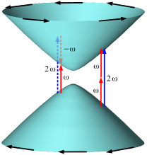
Figure 1: (Color online) One- and two-photon interference processes illustrates on the helical Dirac cone. The one in the left has energy $\hbar\omega$ corresponds to $(i)1$, while the other on the right has energy $2\hbar\omega$ corresponds to $(i)2$.

III Two-band systems

Any Hermitian $2\times 2$ matrix can be written as a linear combination of Pauli matrices $\sigma$ and the identity $\sigma_{0}$. So a generic Hamiltonian for two bands is ${\cal H}=\sum_{\bm{k}}a_{\alpha,\bm{k}}^{\dagger}H_{\alpha\beta,\bm{k}}a_{\beta,\bm{k}}$, where $\alpha,\beta=1,2$ are band indices, and

$$H_{\bm{k}}=\hbar\varpi_{\bm{k}}\sigma_{0}+\hbar\bm{d}_{\bm{k}}\cdot\bm{\sigma}=\hbar\left[\begin{array}[]{cc}\varpi_{\bm{k}}+d_{\bm{k}}^{z}&d_{\bm{k}}^{x}-id_{\bm{k}}^{y}\\ d_{\bm{k}}^{x}+id_{\bm{k}}^{y}&\varpi_{\bm{k}}-d_{\bm{k}}^{z}\end{array}\right]$$ (15)

denotes the Hamiltonian at each lattice momentum $\bm{k}$. The eigenenergies are $E_{\bm{k}\pm}=\hbar\left(\varpi_{\bm{k}}\pm d_{\bm{k}}\right)$ where $d_{\bm{k}}=\left|\bm{d}_{\bm{k}}\right|$, with $\left(+\right)=c$ and $\left(-\right)=v$ representing the conduction and valence bands respectively, so $\omega_{cv,\bm{k}}=2d_{\bm{k}}$. The eigenstates satisfy $\hat{\bm{d}}_{\bm{k}}\cdot\bm{\sigma}\psi_{\bm{k}\pm}=\pm\psi_{\bm{k}\pm}$, so when $\hat{\bm{d}}_{\bm{k}}\cdot\bm{\sigma}$ is diagonalized it is represented by $\sigma_{z}$, and there is a unitary matrix $U_{\bm{k}}$ that performs the change of basis, $\hat{\bm{d}}_{\bm{k}}\cdot\bm{\sigma}=U_{\bm{k}}\sigma_{z}U_{\bm{k}}^{\dagger}$. Because $SU\left(2\right)$ and $SO\left(3\right)$ have the same algebra, we can write $U_{\bm{k}}\sigma_{z}U_{\bm{k}}^{\dagger}=\left({\cal R}_{\bm{k}}\hat{\bm{z}}\right)\cdot\bm{\sigma}$, where ${\cal R}_{\bm{k}}$ represents a rotation around the axis $\hat{\bm{n}}_{\bm{k}}$ by an angle $\phi_{\bm{k}}$, so $U_{\bm{k}}=\exp\left(-i\frac{\phi_{\bm{k}}}{2}\hat{\bm{n}}_{\bm{k}}\cdot\bm{\sigma}\right)$; we put $\hat{\bm{n}}_{\bm{k}}=\hat{\bm{z}}\times\hat{\bm{d}}_{\bm{k}}/\left|\hat{\bm{z}}\times\hat{\bm{d}}_{\bm{k}}\right|$ and $\cos\phi_{\bm{k}}=\hat{z}\cdot\hat{\bm{d}}_{\bm{k}}$. The triad $\left(\hat{\bm{n}}_{\bm{k}},\hat{\bm{d}}_{\bm{k}},\hat{\bm{n}}_{\bm{k}}\times\hat{\bm{d}}_{\bm{k}}\right)$ forms an orthonormal basis, so an arbitrary operator can be written as

$$\begin{array}[]{rl}\hat{\bm{w}}\cdot\bm{\sigma}=&\left(\hat{\bm{n}}_{\bm{k}}\cdot\hat{\bm{w}}\right)\hat{\bm{n}}_{\bm{k}}\cdot\bm{\sigma}+\left(\hat{\bm{d}}_{\bm{k}}\cdot\hat{\bm{w}}\right)\hat{\bm{d}}_{\bm{k}}\cdot\bm{\sigma}\\ &+\left[\left(\hat{\bm{n}}_{\bm{k}}\times\hat{\bm{d}}_{\bm{k}}\right)\cdot\hat{\bm{w}}\right]\left(\hat{\bm{n}}_{\bm{k}}\times\hat{\bm{d}}_{\bm{k}}\right)\cdot\bm{\sigma},\end{array}$$ (16)

and in the basis of eigenvectors

$$\begin{array}[]{rl}U_{\bm{k}}^{\dagger}\left(\hat{\bm{w}}\cdot\bm{\sigma}\right)U_{\bm{k}}=&\left(\hat{\bm{n}}_{\bm{k}}\cdot\hat{\bm{w}}\right)\hat{\bm{n}}_{\bm{k}}\cdot\bm{\sigma}+\left(\hat{\bm{d}}_{\bm{k}}\cdot\hat{\bm{w}}\right)\hat{\bm{z}}\cdot\bm{\sigma}\\ &+\left[\left(\hat{\bm{n}}_{\bm{k}}\times\hat{\bm{d}}_{\bm{k}}\right)\cdot\hat{\bm{w}}\right]\left(\hat{\bm{n}}_{\bm{k}}\times\hat{\bm{z}}\right)\cdot\bm{\sigma},\end{array}$$ (17)

which allows any operator to be expressed simply.

Operators

The quantities of interest are the densities of injected carriers $\left\langle n\right\rangle$, spin $\left\langle\bm{S}\right\rangle$, charge current $\left\langle\bm{J}_{c}\right\rangle$ and spin current $\left\langle\bm{J}_{S}\right\rangle$, which are computed below.

We keep track of the injected carriers by computing the density of electrons injected into the conduction band. The corresponding number operator has matrix elements $n_{cc}=1$ and $n_{vv}=0$.

We suppose that the components of the spin operator are given by $S^{a}=\frac{\hbar}{2}\hat{\bm{a}}\cdot\bm{\sigma}$, and decompose $\hat{\bm{a}}\cdot\bm{\sigma}$ according to Eq. (17), so

$$\begin{array}[]{rl}S_{cc}^{a}=&\frac{\hbar}{2}{\rm Tr}\left[S^{a}\left(I+\sigma_{z}\right)\right]=\frac{\hbar}{2}\hat{\bm{d}}_{\bm{k}}\cdot\hat{\bm{a}},\\ S_{vv}^{a}=&\frac{\hbar}{2}{\rm Tr}\left[S^{a}\left(I-\sigma_{z}\right)\right]=-\frac{\hbar}{2}\hat{\bm{d}}_{\bm{k}}\cdot\hat{\bm{a}}\end{array}$$ (18)

are the matrix elements needed. Note that even though $S_{cc}^{a}$ and $S_{vv}^{a}$ are matrix elements of the spin operator in the basis of eigenstates, they are being expressed in terms of the parameters of the Hamiltonian in its non-diagonal form of Eq. (15).

The matrix associated with the velocity operator is

$$v_{\bm{k}}^{a}=\frac{1}{\hbar}\partial_{k^{a}}H_{\bm{k}}=\partial_{k^{a}}\varpi_{\bm{k}}\sigma_{0}+\partial_{k^{a}}\bm{d}_{\bm{k}}\cdot\bm{\sigma},$$ (19)

and decomposing it according to Eq. (17) gives

$$\begin{array}[]{rl}v_{\bm{k}}^{a}=&\partial_{k^{a}}\varpi_{\bm{k}}\sigma_{0}+\partial_{k^{a}}d_{\bm{k}}\sigma_{z}+d_{\bm{k}}\left(\hat{\bm{n}}_{\bm{k}}\cdot\partial_{k^{a}}\hat{\bm{d}}_{\bm{k}}\right)\hat{\bm{n}}_{\bm{k}}\cdot\sigma\\ &+d_{\bm{k}}\left[\left(\hat{\bm{n}}_{\bm{k}}\times\hat{\bm{d}}_{\bm{k}}\right)\cdot\partial_{k^{a}}\hat{\bm{d}}_{\bm{k}}\right]\left(\hat{\bm{n}}_{\bm{k}}\times\hat{\bm{z}}\right)\cdot\sigma.\end{array}$$ (20)

The velocity matrix elements are

$$\begin{array}[]{rl}v_{cc}^{a}=&\partial_{k^{a}}\varpi_{\bm{k}}+\partial_{k^{a}}d_{\bm{k}},\\ v_{vv}^{a}=&\partial_{k^{a}}\varpi_{\bm{k}}-\partial_{k^{a}}d_{\bm{k}},\\ v_{cv}^{a}=&d_{\bm{k}}\left(\hat{\bm{n}}_{\bm{k}}+i\hat{\bm{n}}_{\bm{k}}\times\hat{\bm{d}}_{\bm{k}}\right)\cdot\left(\partial_{k^{a}}\hat{\bm{d}}_{\bm{k}}\right)\hat{\bm{n}}_{\bm{k}}\cdot\left(\hat{\bm{x}}-i\hat{\bm{y}}\right),\\ v_{vc}^{a}=&d_{\bm{k}}\left(\hat{\bm{n}}_{\bm{k}}-i\hat{\bm{n}}_{\bm{k}}\times\hat{\bm{d}}_{\bm{k}}\right)\cdot\left(\partial_{k^{a}}\hat{\bm{d}}_{\bm{k}}\right)\hat{\bm{n}}_{\bm{k}}\cdot\left(\hat{\bm{x}}+i\hat{\bm{y}}\right).\end{array}$$ (21)

It is also necessary to compute products of two velocity matrix elements,

$$v_{cv}^{a}v_{vc}^{b}=d_{\bm{k}}^{2}\left[\partial_{k^{a}}\hat{\bm{d}}_{\bm{k}}\cdot\partial_{k^{b}}\hat{\bm{d}}_{\bm{k}}+i\hat{\bm{d}}_{\bm{k}}\cdot\left(\partial_{k^{a}}\hat{\bm{d}}_{\bm{k}}\times\partial_{k^{b}}\hat{\bm{d}}_{\bm{k}}\right)\right].$$ (22)

The second term above is the Berry curvature; we can track the contributions to optical properties that depend on it. The charge current is expressed in terms of the velocity operator by $\bm{J}=e\bm{v}$.

We define the spin current operator as $J_{S,\bm{k}}^{ab}=\frac{1}{2}\left(S^{a}v_{\bm{k}}^{b}+v_{\bm{k}}^{b}S^{a}\right)$ so for a system where $S^{a}=\frac{\hbar}{2}\hat{\bm{a}}\cdot\bm{\sigma}$ we have

$$\begin{array}[]{rl}U_{\bm{k}}^{\dagger}J_{S,\bm{k}}^{ab}U_{\bm{k}}=&\frac{\hbar}{2}\left[\hat{\bm{a}}\cdot\hat{\bm{d}}_{\bm{k}}\left(\partial_{k^{b}}d_{\bm{k}}\right)+d_{\bm{k}}\left(\hat{\bm{a}}\cdot\partial_{k^{b}}\hat{\bm{d}}_{\bm{k}}\right)\right]+\\ &+\left(\partial_{k^{b}}\varpi_{\bm{k}}\right)U_{\bm{k}}^{\dagger}S^{a}U_{\bm{k}},\end{array}$$ (23)

and the components are

$$\begin{array}[]{rl}J_{S,cc}^{ab}=&\hbar\frac{\hat{\bm{a}}\cdot\hat{\bm{d}}_{\bm{k}}\left(\partial_{k^{b}}d_{\bm{k}}\right)+d_{\bm{k}}\hat{\bm{a}}\cdot\partial_{k^{b}}\hat{\bm{d}}_{\bm{k}}+\left(\partial_{k^{b}}\varpi_{\bm{k}}\right)\hat{\bm{a}}\cdot\hat{\bm{d}}_{\bm{k}}}{2},\\ J_{S,vv}^{ab}=&\hbar\frac{\hat{\bm{a}}\cdot\hat{\bm{d}}_{\bm{k}}\left(\partial_{k^{b}}d_{\bm{k}}\right)+d_{\bm{k}}\hat{\bm{a}}\cdot\partial_{k^{b}}\hat{\bm{d}}_{\bm{k}}-\left(\partial_{k^{b}}\varpi_{\bm{k}}\right)\hat{\bm{a}}\cdot\hat{\bm{d}}_{\bm{k}}}{2},\end{array}$$ (24)

which completes the list of necessary matrix elements.

Optical injection coefficients

The quantities necessary for computing the injection rates are readily obtained from the equations above, giving

$$\begin{array}[]{rl}\Omega_{cv,\bm{k}}^{bc}\left(\omega_{\alpha}\right)=&\frac{-e^{2}}{\hbar^{2}\omega^{2}}\left(\frac{v_{cc}^{b}v_{cv}^{c}}{\omega_{\alpha}-\omega_{cv}}+\frac{v_{cv}^{b}v_{vv}^{c}}{\omega_{\alpha}}\right),\\ {\cal W}_{cv,\bm{k}}^{bc}\left(\omega_{\alpha},\omega_{\beta}\right)=&\frac{e^{2}}{\hbar^{2}\omega^{2}}\left[\frac{v_{cv}^{b}\partial_{k^{c}}d_{\bm{k}}}{\omega_{\alpha}}+\frac{v_{cv}^{c}\partial_{k^{b}}d_{\bm{k}}}{\omega_{\beta}}\right],\end{array}$$ (25)

where we have used the fact that $\omega_{\alpha}+\omega_{\beta}=\omega_{cv}$. Therefore

$$\begin{array}[]{rl}\Gamma_{1,cv}^{bc}\left(\bm{k},\omega\right)=&\frac{e^{2}d_{\bm{k}}^{2}\left[\partial_{k^{b}}\hat{\bm{d}}_{\bm{k}}\cdot\partial_{k^{c}}\hat{\bm{d}}_{\bm{k}}-i\hat{\bm{d}}_{\bm{k}}\cdot\left(\partial_{k^{b}}\hat{\bm{d}}_{\bm{k}}\times\partial_{k^{c}}\hat{\bm{d}}_{\bm{k}}\right)\right]}{\hbar^{2}\omega^{2}},\\ \Gamma_{2,cv}^{bcde}\left(\bm{k},\omega\right)=&\frac{e^{4}}{\hbar^{4}\omega^{4}}\left[\frac{v_{cv}^{d}\partial_{k^{e}}d_{\bm{k}}+v_{cv}^{e}\partial_{k^{d}}d_{\bm{k}}}{\omega}\right]\left[\frac{v_{vc}^{b}\partial_{k^{c}}d_{\bm{k}}+v_{vc}^{c}\partial_{k^{b}}d_{\bm{k}}}{\omega}\right],\end{array}$$ (26)

and

$$\begin{array}[]{rl}\Gamma_{i\left(1\right),cv}^{bcd}\left(\bm{k},\omega\right)=&\frac{ie^{3}}{\hbar^{3}\omega^{3}}\left[\frac{v_{cv}^{c}v_{vc}^{b}\partial_{k^{d}}d_{\bm{k}}}{2\omega}-\frac{v_{cv}^{d}v_{vc}^{b}\partial_{k^{c}}d_{\bm{k}}}{\omega}\right],\\ \Gamma_{i\left(2\right),cv}^{bcd}\left(\bm{k},\omega\right)=&\frac{ie^{3}}{2\hbar^{3}\omega^{3}}\left[\frac{v_{cv}^{d}v_{vc}^{b}\partial_{k^{c}}d_{\bm{k}}+v_{cv}^{d}v_{vc}^{c}\partial_{k^{b}}d_{\bm{k}}}{\omega}\right].\end{array}$$ (27)

For a two-band system there is only one valence and one conduction band, $c^{\prime}=c$ and $v^{\prime}=v$, so Eqs. (13) and (14) become simpler; in the continuum limit the momentum sums are expressed by

$$\begin{array}[]{rl}\Lambda_{1}^{bc}\left(n\omega\right)=&\underset{\omega_{cv}=n\omega}{\int}\frac{\left(dk\right)^{D-1}}{\left(2\pi\right)^{D-1}}\frac{\left(M_{cc,\bm{k}}-M_{vv,\bm{k}}\right)\Gamma_{1,cv}^{bc}\left(\bm{k},n\omega\right)}{\left|\bm{\nabla}_{\bm{k}}\omega_{cv}\right|},\\ \Lambda_{2}^{bcde}\left(\omega\right)=&\underset{\omega_{cv}=2\omega}{\int}\frac{\left(dk\right)^{D-1}}{\left(2\pi\right)^{D-1}}\frac{\left(M_{cc,\bm{k}}-M_{vv,\bm{k}}\right)\Gamma_{2,cv}^{bcde}\left(\bm{k},\omega\right)}{\left|\bm{\nabla}_{\bm{k}}\omega_{cv}\right|},\\ \Lambda_{i\left(n\right)}^{bcd}\left(\omega\right)=&\underset{\omega_{cv}=n\omega}{\int}\frac{\left(dk\right)^{D-1}}{\left(2\pi\right)^{D-1}}\frac{\left(M_{cc,\bm{k}}-M_{vv,\bm{k}}\right)\Gamma_{i,cv,\left(n\right)}^{bcd}\left(\bm{k},\omega\right)}{\left|\bm{\nabla}_{\bm{k}}\omega_{cv}\right|},\end{array}$$ (28)

where each $D-1$ dimensional integral is over the region specified by the energy matching condition $\omega_{cv}=n\omega$.

IV Topological insulators

When the photon energy is smaller than the bulk band gap of a topological insulators, only the protected states localized on their surfaces will contribute to the optical absorption and injection.

The standard effective model obtained from a $\bm{k}\cdot\bm{p}$ approximation for the materials in the family of BiSeTe results in a four-band Hamiltonian liu10

$$H_{\bm{k}}=\varepsilon_{\bm{k}}^{0}I_{4\times 4}+\hbar\left[\begin{array}[]{cccc}m_{\bm{k}}&A_{1}k_{z}&0&A_{2}k_{-}\\ A_{1}k_{z}&-m_{\bm{k}}&A_{2}k_{-}&0\\ 0&A_{2}k_{+}&m_{\bm{k}}&-A_{1}k_{z}\\ A_{2}k_{+}&0&-A_{1}k_{z}&-m_{\bm{k}}\end{array}\right],$$ (29)

where $k_{\pm}=k_{x}\pm ik_{y}$, $\varepsilon_{k}^{0}=C+D_{1}k_{z}^{2}+D_{2}k_{\perp}^{2}$ and $m_{\bm{k}}=m-B_{1}k_{z}^{2}-B_{2}k_{\perp}^{2}$ with the constants depending on the material.

In order to consider interfaces along the $\hat{\bm{z}}$ direction one can write the Hamiltonian in a separated form $H_{\bm{k}}=H_{\bm{k}}^{\perp}+H_{\bm{k}}^{z}$, and in the limit of $\bm{k}_{\perp}\to 0$ the transverse part $H_{\bm{k}}^{\perp}$ can be neglected. Also, $H_{\bm{k}}^{z}$ is block diagonal and separates into two sectors according to the spin of the electrons. The boundary conditions for surface states then lead to only one solution for each sector, giving two independent states. Next, the $4\times 4$ bulk Hamiltonian with lattice momentum near the $\Gamma$ point is projected on the subspace spanned by the two independent surface states, and an effective Hamiltonian is obtained for the surface states,

$$H_{\bm{k}_{\perp}}=\hbar\left(C_{0}+D_{0}k^{2}\right)\sigma_{0}-\hbar A_{0}\left(\hat{\bm{z}}\times\bm{k}\right)\cdot\bm{\sigma},$$ (30)

which is valid in the limit of large slab thickness lu10 and including terms up to the second order in $\bm{k}$. The parameters $C_{0}$, $D_{0}$ and $A_{0}$ can be determined in terms of the bulk parameters appearing in Eq. (29).

In order to identify the most basic features of coherent control optical injection in topological insulators we will compute the injection rates starting from the Hamiltonian of Eq. (30). However, in order to keep track of how the Berry curvature effects the optical response we keep a $\sigma_{z}$ mass term that would correspond, for instance, to an external magnetic field along the $\hat{\bm{z}}$ direction. The 2D Hamiltonian we consider is then

$$H_{\bm{k}_{\perp}}=\hbar\left(C_{0}+D_{0}k^{2}\right)\sigma_{0}-\hbar A_{0}\left(\hat{\bm{z}}\times\bm{k}\right)\cdot\bm{\sigma}+\hbar\Delta_{m}\sigma_{z},$$ (31)

which corresponds to Eq. (15) with $\varpi_{\bm{k}}=C_{0}-Dk^{2}$ and $\bm{d}_{\bm{k}}=A_{0}\left(\hat{\bm{z}}\times\bm{k}\right)+\Delta_{m}\hat{\bm{z}}$ so $\hat{\bm{n}}_{\bm{k}}=-\hat{\bm{k}}$ and

$$\begin{array}[]{rl}\partial_{k^{b}}d_{\bm{k}}=&\frac{A_{0}^{2}k^{b}}{d_{\bm{k}}},\\ \partial_{k^{b}}\hat{\bm{d}}_{\bm{k}}=&\frac{-A_{0}\left(\hat{\bm{z}}\times\hat{\bm{b}}\right)}{d_{\bm{k}}}-\frac{A_{0}^{2}k^{b}\hat{\bm{d}}_{\bm{k}}}{d_{\bm{k}}^{2}}.\end{array}$$ (32)

This allows us to compute the optical injection coefficients. Since in the basis of Eq. (30) the spin operator is represented by $S^{a}=\frac{\hbar}{2}\hat{\bm{a}}\cdot\bm{\sigma}$, from Eq. (18), Eq. (21) and Eq. (24) we can identify the matrix elements of the operators of interest

$$\begin{array}[]{rl}S_{cc}^{a}-S_{vv}^{a}=&\hbar\hat{\bm{a}}\cdot\hat{\bm{d}}_{\bm{k}}=\frac{\hbar A_{0}k^{z\times a}+\hbar\Delta_{m}\hat{\bm{z}}\cdot\hat{\bm{a}}}{d_{\bm{k}}},\\ v_{cc}^{a}-v_{vv}^{a}=&2\partial_{k^{a}}d_{\bm{k}}=\frac{2A_{0}^{2}k^{a}}{d_{\bm{k}}},\\ J_{S,cc}^{ab}-J_{S,vv}^{ab}=&\hbar\left(\partial_{k^{b}}\varepsilon_{k}\right)\hat{\bm{a}}\cdot\hat{\bm{d}}_{\bm{k}}=\frac{2\hbar D_{0}k^{b}\left[A_{0}k^{z\times a}+\Delta_{m}\hat{\bm{z}}\cdot\hat{\bm{a}}\right]}{d_{\bm{k}}}.\end{array}$$ (33)

They satisfy the relations

$$\begin{array}[]{rl}S_{cc}^{z}-S_{vv}^{z}=&\frac{\hbar\Delta_{m}}{d_{\bm{k}}}=\frac{\hbar\Delta_{m}}{d_{\bm{k}}}\left(n_{cc}-n_{vv}\right),\vspace{2pt}\\ \bm{v}=&-\frac{2A_{0}\hat{\bm{z}}\times\bm{S}}{\hbar},\vspace{2pt}\\ J_{S,cc}^{zb}-J_{S,vv}^{zb}=&\frac{2\hbar D_{0}k^{b}\Delta_{m}}{d_{\bm{k}}}=\frac{\hbar D_{0}\Delta_{m}}{A_{0}^{2}}\left(v_{cc}^{b}-v_{vv}^{b}\right),\end{array}$$ (34)

where the second equation is the identity explored by Raghu et al. [raghu10, ]; the first states that the $\hat{\bm{z}}$ component of the spin density $S^{z}$ merely corresponds to the spin polarization of the injected carriers; and the third identifies the $\hat{\bm{z}}$ component of the spin current $J_{S}^{z}$ as entirely due to the spin polarization of the charge current. Both spin density and current are non-zero only in the presence of the $\sigma_{z}$ mass $\Delta_{m}$. It should be noted that the spin current is typically not a conserved quantity, and indeed it is not conserved at the surface of topological insulators. Nevertheless, we still compute its optical injection rate because depending on the experimental technique, the spin separation to which it leads might be detected (or tunneled to another material) before the spins relax driel06prl ; driel06ssc .

Eq. (22) is then

$$v_{cv}^{b}v_{vc}^{c}=A_{0}^{2}\hat{\bm{b}}\cdot\hat{\bm{c}}-\frac{A_{0}^{4}k^{b}k^{c}}{d_{\bm{k}}^{2}}+i\frac{A_{0}^{2}\Delta_{m}\hat{\bm{z}}\cdot\left(\hat{\bm{b}}\times\hat{\bm{c}}\right)}{d_{\bm{k}}}$$ (35)

which allows us to compute the $\Gamma$ coefficients of Eq. (26) and Eq. (27), giving

$$\begin{array}[]{rl}\Gamma_{1,cv}^{bc}\left(\bm{k},\omega\right)=&\frac{e^{2}}{\hbar^{2}\omega^{2}}v_{cv}^{c}v_{vc}^{b},\\ \Gamma_{2,cv}^{bcde}\left(\bm{k},\omega\right)=&\frac{e^{4}A_{0}^{4}}{\hbar^{4}\omega^{4}}\left[\frac{k^{e}v_{cv}^{d}+k^{d}v_{cv}^{e}}{\omega d_{\bm{k}}}\right]\left[\frac{k^{c}v_{vc}^{b}+k^{b}v_{vc}^{c}}{\omega d_{\bm{k}}}\right],\end{array}$$ (36)

and

$$\begin{array}[]{rl}\Gamma_{i\left(1\right),cv}^{bcd}\left(\bm{k},\omega\right)=&\frac{ie^{3}A_{0}^{2}}{2\hbar^{3}\omega^{3}}\left[\frac{k^{d}v_{cv}^{c}v_{vc}^{b}-2k^{c}v_{cv}^{d}v_{vc}^{b}}{\omega d_{\bm{k}}}\right],\\ \Gamma_{i\left(2\right),cv}^{bcd}\left(\bm{k},\omega\right)=&\frac{ie^{3}A_{0}^{2}}{2\hbar^{3}\omega^{3}}\left[\frac{k^{c}v_{cv}^{d}v_{vc}^{b}+k^{b}v_{cv}^{d}v_{vc}^{c}}{\omega d_{\bm{k}}}\right].\end{array}$$ (37)

The optical injection coefficients can now be computed.

The only relevant states for our calculations are localized on the surface, so the momentum integrals are all two dimensional. Since $\omega_{cv,\bm{k}}$ does not depend on the direction of the momentum, when the integrals are performed in polar coordinates $\left(k,\theta\right)$, the $k$ integral simply deals with the delta function setting $2d_{\bm{k}}=\omega$ or $2d_{\bm{k}}=2\omega$ depending on the term. So Eq. (28) becomes

$$\begin{array}[]{rl}\Lambda_{1}^{bc}\left(n\omega\right)=&\left.\int\frac{d\theta}{2\pi}\frac{d_{\bm{k}}\left(M_{cc,\bm{k}}-M_{vv,\bm{k}}\right)\Gamma_{1,cv}^{bc}\left(\bm{k},n\omega\right)}{2A_{0}^{2}}\right|_{d_{\bm{k}}=\frac{n\omega}{2}},\\ \Lambda_{2}^{bcde}\left(\omega\right)=&\left.\int\frac{d\theta}{2\pi}\frac{d_{\bm{k}}\left(M_{cc,\bm{k}}-M_{vv,\bm{k}}\right)\Gamma_{2,cv}^{bcde}\left(\bm{k},\omega\right)}{2A_{0}^{2}}\right|_{d_{\bm{k}}=\omega},\\ \Lambda_{i\left(n\right)}^{bcd}\left(\omega\right)=&\left.\int\frac{d\theta}{2\pi}\frac{d_{\bm{k}}\left(M_{cc,\bm{k}}-M_{vv,\bm{k}}\right)\Gamma_{i,cv,\left(n\right)}^{bcd}\left(\bm{k},\omega\right)}{2A_{0}^{2}}\right|_{d_{\bm{k}}=\frac{n\omega}{2}}.\end{array}$$ (38)

The expressions for the various coefficients that follow from these expressions are the main results of this paper, and are detailed in Appendix B.

V Results

For the system we are considering, one- and two-photon absorption processes inject scalar quantities while interference processes inject vectorial ones. We confirm within our model that carriers are injected by one- and two-photon absorption processes, but not from the interference between them. Conversely, charge current is injected solely from the interference processes and not from the one- and two-photon absorption processes. However, there are additional peculiarities for the spin density and spin current injection.

Due to the relations (34), the in-plane spin density follows the charge current injection, stemming only from the interference processes; the out-of-plane spin density only has contributions from the one- and two-photon absorption processes. It simply corresponds to the spin polarization of the injected carriers, which is proportional to the $\sigma_{z}$ mass term in the Hamiltonian.

A similar situation holds for the spin current. The spin current of the $\hat{\bm{z}}$ component of spin follows the charge current and simply amounts to the net spin polarization of the carriers of the current; it is obtained from the interference terms. On the other hand, the in-plane spin current is a result of the Dirac cone with chiral spins; it does not require a net spin polarization generated by a $\sigma_{z}$ mass term. It is obtained from one- and two-photon absorption and has no contribution from interference processes.

Below we present the injection rates for the quantities of interest, considering linear and circular polarizations. In Appendix A we show the general expressions for the optical injection coefficients, and in Appendix B we present the explicit form of the coefficients related to linear and circular polarizations of the incident light, which are referred to below.

The values of the parameters $A_{0}$, $D_{0}$ and $\Delta_{m}=\frac{\mu_{B}g}{2\hbar}B$ used for the plots or specific estimates are given in Table 1; they correspond to the parameters of $Bi_{2}Te_{3}$ for an applied magnetic field around $10T$. liu10

$A_{0}$	$D_{0}$	$\hbar\Delta_{m}$	$E_{\omega}$	$E_{2\omega}$
$5\cdot 10^{5}\frac{m}{s}$	$7\cdot 10^{-4}\frac{m^{2}}{s}$	$1.5\cdot 10^{-2}eV$	$10^{4}\frac{V}{m}$	$72\frac{V}{m}$

Table 1: Values of the parameters used for the plots.

We consider field amplitudes of $E_{\omega}=10^{4}\frac{V}{m}$ for the fundamental and $E_{2\omega}=72\frac{V}{m}$ for the second harmonic, which are indicative of the largest field intensities allowed within the perturbative regime. These values depend on the expressions for the injected carrier density, so we explain how they are obtained in Sec. VI.

V.1 Linear polarizations

The one- and two-photon processes do not depend on the relative orientation of the fundamental $\bm{E}\left(\omega\right)=E_{\omega}e^{i\theta_{1}}\hat{\bm{e}}_{\omega}$ and second harmonic $\bm{E}\left(2\omega\right)=E_{2\omega}e^{i\theta_{2}}\hat{\bm{e}}_{2\omega}$ fields, where $E_{\omega}$ and $E_{2\omega}$ are real. Therefore we show here the results for the injection coefficients $\Lambda_{1}$ and $\Lambda_{2}$, while the results for $\Lambda_{i\left(1\right)}$ and $\Lambda_{i\left(2\right)}$ are displayed for the special cases of parallel and perpendicular polarizations.

The carrier density injection rate is given by

$$\begin{array}[]{rl}\left\langle\dot{n}_{1}\right\rangle=&\xi_{1}^{xx}\left(\omega\right)E_{\omega}^{2}+\xi_{1}^{xx}\left(2\omega\right)E_{2\omega}^{2},\\ \left\langle\dot{n}_{2}\right\rangle=&\xi_{2}^{xxxx}\left(\omega\right)E_{\omega}^{4},\end{array}$$ (39)

and the $\hat{\bm{z}}$ component of the spin density injection rate is given by

$$\begin{array}[]{rl}\left\langle\dot{S}_{1}^{z}\right\rangle=&\frac{2\hbar\Delta_{m}}{\omega}\left[\xi_{1}^{xx}\left(\omega\right)E_{\omega}^{2}+\frac{1}{2}\xi_{1}^{xx}\left(2\omega\right)E_{2\omega}^{2}\right],\\ \left\langle\dot{S}_{2}^{z}\right\rangle=&\frac{\hbar\Delta_{m}}{\omega}\xi_{2}^{xxxx}\left(\omega\right)E_{\omega}^{4}.\end{array}$$ (40)

This result simply corresponds to the net polarization of the injected carriers.

The charge current injection rate vanishes; $\left\langle\dot{J}_{1}^{a}\right\rangle=\left\langle\dot{J}_{2}^{a}\right\rangle=0$.

The spin current injection rate is

$$\begin{array}[]{rl}\left\langle\dot{J}_{S,1}^{ab}\right\rangle=&\underset{n=1,2}{\sum}\left(\hat{\bm{z}}\times\hat{\bm{e}}_{n\omega}\right)\cdot\hat{\bm{a}}\left(\hat{\bm{e}}_{n\omega}\cdot\hat{\bm{b}}\right)\mu_{1}^{yxxx}\left(n\omega\right)E_{n\omega}^{2}+\\ &+\underset{n=1,2}{\sum}\hat{\bm{e}}_{n\omega}\cdot\hat{\bm{a}}\left(\hat{\bm{z}}\times\hat{\bm{e}}_{n\omega}\right)\cdot\hat{\bm{b}}\mu_{1}^{xyxx}\left(n\omega\right)E_{n\omega}^{2},\\ \left\langle\dot{J}_{S,2}^{ab}\right\rangle=&\left(\hat{\bm{z}}\times\hat{\bm{e}}_{n\omega}\right)\cdot\hat{\bm{a}}\left(\hat{\bm{e}}_{n\omega}\cdot\hat{\bm{b}}\right)\mu_{2}^{yxxxxx}\left(\omega\right)E_{\omega}^{4}+\\ &+\hat{\bm{e}}_{\omega}\cdot\hat{\bm{a}}\left(\hat{\bm{z}}\times\hat{\bm{e}}_{\omega}\right)\cdot\hat{\bm{b}}\mu_{2}^{xyxxxx}\left(\omega\right)E_{\omega}^{4},\end{array}$$ (41)

the first term in each equation gives a spin current independent of the applied field polarization, and is due the helical spin structure.

Parallel orientations

Only the interference processes depend on the relative orientation of the $\bm{E}\left(\omega\right)$ and $\bm{E}\left(2\omega\right)$. Here the fields are $\bm{E}\left(\omega\right)=E_{\omega}e^{i\theta_{1}}\hat{\bm{e}}_{\omega}$ and $\bm{E}\left(2\omega\right)=E_{2\omega}e^{i\theta_{2}}\hat{\bm{e}}_{\omega}$. The relative phase parameter is $\Delta\theta=\theta_{2}-2\theta_{1}$.

The charge current injection rate is given by

$$\begin{array}[]{rl}\left\langle\dot{\bm{J}}_{i}\right\rangle=&-2\hat{\bm{e}}_{\omega}{\rm Im}\left[\eta_{i\left(1\right)}^{xxxx}\left(\omega\right)+\eta_{i\left(2\right)}^{xxxx}\left(\omega\right)\right]\\ &\cdot\sin\left(\Delta\theta\right)E_{\omega}^{2}E_{2\omega}.\end{array}$$ (42)

Due to Eq. (34), the in plane spin density and the spin $\hat{\bm{z}}$ current injection rates are given in terms of $\left\langle\dot{\bm{J}}_{i}\left(\omega\right)\right\rangle$ by

$$\begin{array}[]{rl}\left\langle\dot{\bm{S}}_{i}\right\rangle=&\frac{\hbar}{2A_{0}e}\hat{\bm{z}}\times\left\langle\dot{\bm{J}}_{i}\right\rangle,\\ \left\langle\dot{\bm{J}}_{S,i}^{z}\right\rangle=&\frac{\hbar D_{0}\Delta_{m}}{A_{0}^{2}e}\left\langle\dot{\bm{J}}_{i}\right\rangle,\end{array}$$ (43)

the spin current merely corresponds to the magnetization of the carriers of the charge current.

The direction of the polarization vector provides control of the angle of the injected vectorial quantities, while the relative phase parameter of the light beams can control only their magnitude and orientation.

Perpendicular orientations

Here we have $\bm{E}\left(\omega\right)=E_{\omega}e^{i\theta_{1}}\hat{\bm{e}}_{\omega}$ and $\bm{E}\left(2\omega\right)=E_{2\omega}e^{i\theta_{2}}\hat{\bm{e}}_{2\omega}$ with $\hat{\bm{e}}_{2\omega}=\hat{\bm{z}}\times\hat{\bm{e}}_{\omega}$. The relative phase parameter is again $\Delta\theta=\theta_{2}-2\theta_{1}$.

The charge current injection rate is given by

$$\begin{array}[]{rl}\left\langle\dot{J}_{i}^{a}\right\rangle=&-2\hat{\bm{e}}_{2\omega}\cdot\hat{\bm{a}}{\rm Im}\left[\eta_{i\left(1\right)}^{yxxy}\left(\omega\right)+\eta_{i\left(2\right)}^{yxxy}\left(\omega\right)\right]\\ &\cdot\sin\left(\Delta\theta\right)E_{\omega}^{2}E_{2\omega}\\ &+2\hat{\bm{e}}_{\omega}\cdot\hat{\bm{a}}{\rm Re}\left[\eta_{i\left(1\right)}^{xxxy}\left(\omega\right)+\eta_{i\left(2\right)}^{xxxy}\left(\omega\right)\right]\\ &\cdot\cos\left(\Delta\theta\right)E_{\omega}^{2}E_{2\omega},\end{array}$$ (44)

and the spin density and current follow Eq. (43).

From Eqs. (65) and (66) in Appendix B we can identify two different contributions to the injection: one that is related to the Berry curvature, and thus depends on $\Delta_{m}$, and another that is independent of $\Delta_{m}$.

Again the direction of the polarization vector provides control of the angle of the injected vectorial quantities. The relative phase can still control their magnitude and orientation, but it can also switch between the two regimes: the first where the photoinjection stems from the Berry curvature, and the second where it does not.

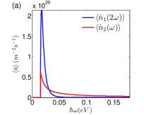
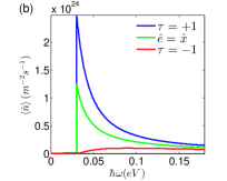
Figure 2: (Color online) (a) Carrier density injection rates from one- and two-photon absorption processes at total energy $2\hbar\omega$. (b) Carrier density injection rates for linear($\hat{\bm{e}}_{\omega}=\hat{\bm{x}}$) and circular($\tau=\pm 1$) polarizations of the incident fields.

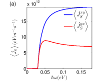
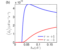
Figure 3: (Color online) Planar spin current density injection rates for (a) linear polarizations along the $\hat{\bm{x}}$ direction and (b) circular polarizations.

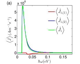
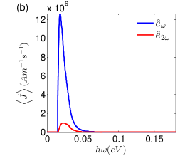
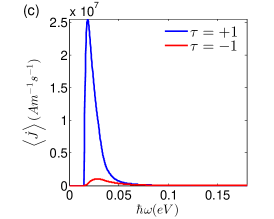
Figure 4: (Color online) Current density injection rates for (a) linear polarizations with parallel orientations (b) linear polarizations with perpendicular orientations, showing the components of the current along the $\hat{\bm{e}}_{\omega}$ and $\hat{\bm{e}}_{2\omega}$ directions, and (c) circular polarizations.

V.2 Circular polarizations

For circular polarizations $\bm{E}\left(\omega\right)=E_{\omega}e^{i\theta_{1}}\hat{\bm{p}}_{\tau_{1}}$ and $\bm{E}\left(2\omega\right)=E_{2\omega}e^{i\theta_{2}}\hat{\bm{p}}_{\tau_{2}}$ where $\tau_{1},\tau_{2}=\pm 1$ and $\hat{\bm{p}}_{\pm}=\left(\hat{\bm{x}}\pm i\hat{\bm{y}}\right)/\sqrt{2}$, so $\hat{\bm{p}}_{\tau}\cdot\hat{\bm{p}}_{\tau}=0$ and $\hat{\bm{p}}_{+}\cdot\hat{\bm{p}}_{-}=1$ as well as $\hat{\bm{p}}_{-}\times\hat{\bm{p}}_{+}=i\hat{\bm{z}}$. The relative phase parameter is still $\Delta\theta=\theta_{2}-2\theta_{1}$. Again the one and two photons processes do not depend on the relative helicity of the $\bm{E}\left(\omega\right)$ and $\bm{E}\left(2\omega\right)$ fields and are presented first.

The carrier density injection rate is now given by

$$\begin{array}[]{rl}\left\langle\dot{n}_{1}\right\rangle=&\xi_{1}^{-+}\left(\omega\right)E_{\omega}^{2}+\xi_{1}^{-+}\left(2\omega\right)E_{2\omega}^{2},\\ \left\langle\dot{n}_{2}\right\rangle=&\xi_{2}^{--++}\left(\omega\right)E_{\omega}^{4}.\end{array}$$ (45)

The spin density injection is still given by Eq. (40), and for the spin current we have

$$\begin{array}[]{rl}\left\langle\dot{J}_{S,1}^{ab}\right\rangle=&2i\left(\hat{\bm{a}}\times\hat{\bm{b}}\right)\cdot\hat{\bm{z}}\underset{n=1,2}{\sum}\mu_{1}^{-+-+}\left(n\omega\right)E_{n\omega}^{2},\\ \left\langle\dot{J}_{S,2}^{ab}\right\rangle=&2i\left(\hat{\bm{a}}\times\hat{\bm{b}}\right)\cdot\hat{\bm{z}}\mu_{2}^{-+--++}\left(\omega\right)E_{\omega}^{4}.\end{array}$$ (46)

Circularly polarized light does not break rotational symmetry, therefore the second term of Eq. (41) is not present.

Equal helicities

The interference processes depend on the relative helicity of the two fields. We first consider the fields with the same helicity, $\bm{E}\left(\omega\right)=E_{\omega}e^{i\theta_{1}}\hat{\bm{p}}_{\tau}$ and $\bm{E}\left(2\omega\right)=E_{2\omega}e^{i\theta_{2}}\hat{\bm{p}}_{\tau}$.

The charge current injection rate is given by

$$\begin{array}[]{rl}\left\langle\dot{J}_{i}^{a}\right\rangle=&2\left[a^{y}\cos\left(\Delta\theta\right)+a^{x}\sin\left(\Delta\theta\right)\right]\\ &\cdot i\left[\eta_{i\left(1\right)}^{+--+}\left(\omega\right)+\eta_{i\left(2\right)}^{+--+}\left(\omega\right)\right]E_{\omega}^{2}E_{2\omega}.\end{array}$$ (47)

The spin density and current follows Eq. (43).

The relative phase displacement between the two light beams can now control the direction of the injected quantities.

Especially for frequencies near the gap, the injection rates for different helicities $\tau$ depend strongly on the chirality of the electronic states, identified by $\Delta_{m}/\left|\Delta_{m}\right|$. The helicity of the incident light has no effect for vanishing $\Delta_{m}$.

Opposite helicities

Here we have $\bm{E}\left(\omega\right)=E_{\omega}e^{i\theta_{1}}\hat{\bm{p}}_{\tau}$ and $\bm{E}\left(2\omega\right)=E_{2\omega}e^{i\theta_{2}}\hat{\bm{p}}_{-\tau}$. The injection rates from interference all vanish for the four operators of interest.

VI Discussion

In order to determine the validity our calculations for the optical injection rates, we have to consider the fraction of the injected carrier population relative to the total number of states in the range of energies covered by the laser pulse. The duration of the pulse $\cal{T}$ sets the frequency broadening of the laser $\Delta\omega=\frac{2\pi}{\cal T}$, which in turn - via the dispersion relation, which we assume $E_{\bm{k}}=\hbar A_{0}k$ here for simplicity - determines the area of the Brillouin zone that can be populated by carriers $a=2\pi k\Delta k$, where $k=\frac{\omega}{A_{0}}$ and $\Delta k=\frac{\Delta\omega}{A_{0}}$. The number of states available in this area of the Brillouin zone is $a/a_{1}$, where $a_{1}=\frac{\left(2\pi\right)^{2}}{L^{2}}$ is the area occupied by one state. The maximum amplitudes of the laser fields are restricted by the condition that the number of injected carriers with additional energy $2\hbar\omega$ is at most $5\%$ of the total number of carrier states in the allowed energy range

$$\left(\xi_{1}^{xx}\left(2\omega\right)E_{2\omega}^{2}+\xi_{2}^{xxxx}\left(\omega\right)E_{\omega}^{4}\right){\cal T}L^{2}<0.05\frac{a}{a_{1}}.$$ (48)

We then estimate the amplitudes by imposing the additional condition $\xi_{1}^{xx}\left(2\omega\right)E_{2\omega}^{2}=\xi_{2}^{xxxx}\left(\omega\right)E_{\omega}^{4}$, which gives optimal interference between the absorption processes rioux12 . Finally, the field amplitudes are limited by

$$\left(eE_{2\omega}\right)^{2}=\frac{4A_{0}^{2}\left(eE_{\omega}\right)^{4}}{\hbar^{2}\omega^{4}}<\frac{1.6\hbar^{2}\omega^{2}}{A_{0}^{2}{\cal T}^{2}}.$$ (49)

For pulses lasting $1ns$ with a frequency of $30meV$, the field amplitudes found are $E_{\omega}=10^{4}\frac{V}{m}$ for the fundamental and $E_{2\omega}=72\frac{V}{m}$ for the second harmonic, which correspond to laser intensities of $9.9\frac{W}{cm^{2}}$ and $0.65\frac{mW}{cm^{2}}$, respectively. We use these values for all $\hbar\omega$ in Figs. 2,3, and 4, although for $\hbar\omega<30meV$ smaller amplitudes would be required to guarantee Eq. (48), and could be found by using Eq. (49).

In the absence of the $\sigma_{z}$ mass term, the carrier and charge current injection rates are very similar to the ones found for graphene rioux11 , except for the adjustments due to having only one Dirac cone and a smaller Fermi velocity. However, even in this case there is also injection of the transverse spin following the same form of the injected current, a signature characteristic of topological insulators. The magnitude of these injected quantities are also of the same order of the values for graphene, which has already been measured norris10 .

Another distinctive trait shared with graphene is the relatively low average velocity of the injected carriers when compared to semiconductors. This is due to the one photon absorption at the fundamental frequency, forbidden in semiconductors because of the bandgap. This gives rise to the extra interference process with total energy $\hbar\omega$, which usually partially cancels the injected current stemming from the interference process with total energy $2\hbar\omega$.

Several particular features are found in the presence of the Berry phase inducing $\Delta_{m}\sigma_{z}$ term, especially for circular polarizations of the optical fields, when an interesting interplay between the helicity $\tau$ of the incident fields and the chirality $\Delta_{m}/\left|\Delta_{m}\right|$ of the Dirac cone can greatly suppress or enhance optical injection. In order to observe these features a combination of high magnetic field and low temperature is necessary. Because the Zeeman coupling $\hbar\Delta_{m}=\frac{\mu_{B}g}{2}B$ needs to be above temperature $k_{B}T$. We estimate that $77K$ and $6T$ should be enough for $Bi_{2}Te_{3}$. For a pronounced effect, the photon energy should not be much larger than the Zeeman gap. Reasonable photon energies for the fundamental field would not be much larger than $\hbar\omega=30meV$, which can be achieved with quantum cascade lasers.

When lasers of similar intensity are considered, the magnitude of the injected currents obtained from coherent control seem to be considerably larger than the values found by other approaches, like applying an in-plane magnetic field or oblique incidence. Therefore it can play a crucial role in the quest for harnessing the exotic properties of topological insulators for spintronic applications.

Appendix A General expressions for the optical injection coefficients

In order to evaluate the coefficients in Eq. (38), the following integrals are helpful

$$\begin{array}[]{rl}\varphi^{ab}=&\int\frac{d\theta}{2\pi}\frac{k^{a}k^{b}}{k^{2}}=\frac{\hat{\bm{a}}\cdot\hat{\bm{b}}}{2},\\ \varphi^{abcd}=&\int\frac{d\theta}{2\pi}\frac{k^{a}k^{b}k^{c}k^{d}}{k^{4}}=\frac{\hat{\bm{a}}\cdot\hat{\bm{b}}\left(\hat{\bm{c}}\cdot\hat{\bm{d}}\right)+\hat{\bm{a}}\cdot\hat{\bm{c}}\left(\hat{\bm{b}}\cdot\hat{\bm{d}}\right)+\hat{\bm{a}}\cdot\hat{\bm{d}}\left(\hat{\bm{b}}\cdot\hat{\bm{c}}\right)}{8},\\ \varphi^{abcdef}=&\int\frac{d\theta}{2\pi}\frac{k^{a}k^{b}k^{c}k^{d}k^{e}k^{f}}{k^{6}}=\underset{pairings}{\sum}\frac{\hat{\bm{a}}\cdot\hat{\bm{b}}\left(\hat{\bm{c}}\cdot\hat{\bm{d}}\right)\hat{\bm{e}}\cdot\hat{\bm{f}}}{48},\end{array}$$ (50)

and

$$\begin{array}[]{rl}\int\frac{d\theta}{2\pi}v_{cv}^{c}v_{vc}^{b}=&\frac{A_{0}^{2}\left(d_{\bm{k}}^{2}+\Delta_{m}^{2}\right)\hat{\bm{c}}\cdot\hat{\bm{b}}}{2d_{\bm{k}}^{2}}+i\frac{A_{0}^{2}\Delta_{m}\hat{\bm{z}}\cdot\left(\hat{\bm{c}}\times\hat{\bm{b}}\right)}{d_{\bm{k}}},\\ \int\frac{d\theta}{2\pi}k^{a}v_{cv}^{c}v_{vc}^{b}=&0,\end{array}$$ (51)

also

$$\begin{array}[]{rl}\int\frac{d\theta}{2\pi}k^{d}k^{b}v_{cv}^{c}v_{vc}^{e}=&\frac{\left(d_{\bm{k}}^{2}-\Delta_{m}^{2}\right)\left[d_{\bm{k}}^{2}\hat{\bm{c}}\cdot\hat{\bm{e}}\left(\hat{\bm{d}}\cdot\hat{\bm{b}}\right)-2\left(d_{\bm{k}}^{2}-\Delta_{m}^{2}\right)\varphi^{bcde}\right]}{2d_{\bm{k}}^{2}}\\ &+i\frac{\left(d_{\bm{k}}^{2}-\Delta_{m}^{2}\right)\Delta_{m}\hat{\bm{d}}\cdot\hat{\bm{b}}\left(\hat{\bm{c}}\times\hat{\bm{e}}\right)\cdot\hat{\bm{z}}}{2d_{\bm{k}}},\end{array}$$ (52)

and

$$\begin{array}[]{rl}\int\frac{d\theta}{2\pi}k^{c}k^{d}k^{e}v_{cv}^{a}v_{vc}^{b}=&0,\\ \int\frac{d\theta}{2\pi}k^{c}k^{d}k^{e}k^{f}v_{cv}^{a}v_{vc}^{b}=&\frac{\left(d_{\bm{k}}^{2}-\Delta_{m}^{2}\right)^{2}\left[d_{\bm{k}}^{2}\hat{\bm{a}}\cdot\hat{\bm{b}}\varphi^{cdef}-\left(d_{\bm{k}}^{2}-\Delta_{m}^{2}\right)\varphi^{abcdef}\right]}{A_{0}^{2}d_{\bm{k}}^{2}}\\ &+i\frac{\left(d_{\bm{k}}^{2}-\Delta_{m}^{2}\right)^{2}\Delta_{m}\left(\hat{\bm{a}}\times\hat{\bm{b}}\right)\cdot\hat{\bm{z}}\varphi^{cdef}}{A_{0}^{2}d_{\bm{k}}}.\end{array}$$ (53)

The above equations combined with Eq. (33), Eq. (35), Eq. (36) and Eq. (37) gives the following results.

One and two photon absorption

The carrier density coefficients are

$$\begin{array}[]{rl}\xi_{1}^{bc}\left(\omega\right)=&\frac{\Theta\left(\omega-2\Delta_{m}\right)e^{2}}{2\hbar^{2}\omega}\left[\frac{\hat{\bm{b}}\cdot\hat{\bm{c}}}{4}\left(1+\frac{4\Delta_{m}^{2}}{\omega^{2}}\right)-i\frac{\Delta_{m}\hat{\bm{z}}\cdot\left(\hat{\bm{b}}\times\hat{\bm{c}}\right)}{\omega}\right],\\ \xi_{2}^{bcde}\left(\omega\right)=&\frac{\Theta\left(\omega-\Delta_{m}\right)e^{4}A_{0}^{2}}{\hbar^{4}\omega^{5}}\left(1-\frac{\Delta_{m}^{2}}{\omega^{2}}\right)\left(\left[\frac{\left(\hat{\bm{b}}\cdot\hat{\bm{d}}\right)\hat{\bm{c}}\cdot\hat{\bm{e}}+\left(\hat{\bm{b}}\cdot\hat{\bm{e}}\right)\hat{\bm{c}}\cdot\hat{\bm{d}}}{2}-2\varphi^{bcde}\left(1-\frac{\Delta_{m}^{2}}{\omega^{2}}\right)\right]+i\frac{\Delta_{m}}{\omega}\left[\frac{\hat{\bm{c}}\cdot\hat{\bm{e}}\left(\hat{\bm{d}}\times\hat{\bm{b}}\right)\cdot\hat{\bm{z}}+\hat{\bm{b}}\cdot\hat{\bm{e}}\left(\hat{\bm{d}}\times\hat{\bm{c}}\right)\cdot\hat{\bm{z}}+\hat{\bm{c}}\cdot\hat{\bm{d}}\left(\hat{\bm{e}}\times\hat{\bm{b}}\right)\cdot\hat{\bm{z}}+\hat{\bm{d}}\cdot\hat{\bm{b}}\left(\hat{\bm{e}}\times\hat{\bm{c}}\right)\cdot\hat{\bm{z}}}{4}\right]\right).\end{array}$$ (54)

The charge current coefficients vanish, $\eta_{1}^{abc}\left(\omega\right)=\eta_{2}^{abcde}\left(\omega\right)=0$.

The spin density coefficients can be written in terms of the carrier density ones as

$$\begin{array}[]{rl}\zeta_{1}^{abc}\left(\omega\right)=&\frac{2\hbar\Delta_{m}\left(\hat{\bm{z}}\cdot\hat{\bm{a}}\right)}{\omega}\xi_{1}^{bc}\left(\omega\right),\\ \zeta_{2}^{abcde}\left(\omega\right)=&\frac{\hbar\Delta_{m}\left(\hat{\bm{z}}\cdot\hat{\bm{a}}\right)}{\omega}\xi_{2}^{bcde}\left(\omega\right),\end{array}$$ (55)

which is a consequence of Eq. (34).

And the spin current coefficients are

$$\begin{array}[]{rl}\mu_{1}^{abcd}\left(\omega\right)=&\frac{\Theta\left(\omega-2\Delta_{m}\right)e^{2}D_{0}}{4A_{0}\hbar}\left(1-\frac{4\Delta_{m}^{2}}{\omega^{2}}\right)\left[\frac{\left(\hat{\bm{z}}\times\hat{\bm{a}}\right)\cdot\hat{\bm{b}}\left(\hat{\bm{c}}\cdot\hat{\bm{d}}\right)}{2}-\varphi^{\left(z\times a\right)bcd}\left(1-\frac{4\Delta_{m}^{2}}{\omega^{2}}\right)+i\frac{\Delta_{m}\left(\hat{\bm{z}}\times\hat{\bm{a}}\right)\cdot\hat{\bm{b}}\left(\hat{\bm{d}}\times\hat{\bm{c}}\right)\cdot\hat{\bm{z}}}{\omega}\right],\\ \mu_{2}^{abcdef}\left(\omega\right)=&\frac{4\Theta\left(\omega-\Delta_{m}\right)e^{4}D_{0}A_{0}}{\hbar^{3}\omega^{4}}\left(1-\frac{\Delta_{m}^{2}}{\omega^{2}}\right)^{2}\left[\frac{\varphi^{\left(z\times a\right)bdf}\hat{\bm{c}}\cdot\hat{\bm{e}}+\varphi^{\left(z\times a\right)bcf}\hat{\bm{d}}\cdot\hat{\bm{e}}+\varphi^{\left(z\times a\right)bde}\hat{\bm{c}}\cdot\hat{\bm{f}}+\varphi^{\left(z\times a\right)bce}\hat{\bm{d}}\cdot\hat{\bm{f}}}{4}-\varphi^{\left(z\times a\right)bcdef}\left(1-\frac{\Delta_{m}^{2}}{\omega^{2}}\right)\right]\\ &+i\frac{4\Theta\left(\omega-\Delta_{m}\right)e^{4}D_{0}A_{0}}{\hbar^{3}\omega^{4}}\frac{\Delta_{m}}{\omega}\left(1-\frac{\Delta_{m}^{2}}{\omega^{2}}\right)^{2}\left[\frac{\varphi^{\left(z\times a\right)bdf}\left(\hat{\bm{e}}\times\hat{\bm{c}}\right)\cdot\hat{\bm{z}}+\varphi^{\left(z\times a\right)bcf}\left(\hat{\bm{e}}\times\hat{\bm{d}}\right)\cdot\hat{\bm{z}}+\varphi^{\left(z\times a\right)bde}\left(\hat{\bm{f}}\times\hat{\bm{c}}\right)\cdot\hat{\bm{z}}+\varphi^{\left(z\times a\right)bce}\left(\hat{\bm{f}}\times\hat{\bm{d}}\right)\cdot\hat{\bm{z}}}{4}\right],\end{array}$$ (56)

giving spin currents with only in-plane components of spin, which is independent of the $\Delta_{m}\sigma_{z}$ mass term.

Interference processes

The carrier density coefficients vanish $\xi_{i\left(n\right)}^{bcd}\left(\omega\right)=0$. The charge current coefficients are

$$\begin{array}[]{rl}\eta_{i\left(1\right)}^{abcd}\left(\omega\right)=&\frac{i\Theta\left(\omega-2\Delta_{m}\right)e^{4}A_{0}^{2}}{4\hbar^{3}\omega^{3}}\left(1-\frac{4\Delta_{m}^{2}}{\omega^{2}}\right)\left(\left[\frac{\left(\hat{\bm{a}}\cdot\hat{\bm{d}}\right)\hat{\bm{b}}\cdot\hat{\bm{c}}-2\left(\hat{\bm{a}}\cdot\hat{\bm{c}}\right)\hat{\bm{b}}\cdot\hat{\bm{d}}}{2}+\varphi^{abcd}\left(1-\frac{4\Delta_{m}^{2}}{\omega^{2}}\right)\right]+i\frac{2\Delta_{m}}{\omega}\left[\frac{\hat{\bm{a}}\cdot\hat{\bm{d}}\left(\hat{\bm{c}}\times\hat{\bm{b}}\right)\cdot\hat{\bm{z}}-2\hat{\bm{a}}\cdot\hat{\bm{c}}\left(\hat{\bm{d}}\times\hat{\bm{b}}\right)\cdot\hat{\bm{z}}}{2}\right]\right),\\ \eta_{i\left(2\right)}^{abcd}\left(\omega\right)=&\frac{i\Theta\left(\omega-\Delta_{m}\right)e^{4}A_{0}^{2}}{2\hbar^{3}\omega^{3}}\left(1-\frac{\Delta_{m}^{2}}{\omega^{2}}\right)\left(\left[\frac{\left(\hat{\bm{a}}\cdot\hat{\bm{c}}\right)\hat{\bm{b}}\cdot\hat{\bm{d}}+\left(\hat{\bm{a}}\cdot\hat{\bm{b}}\right)\hat{\bm{c}}\cdot\hat{\bm{d}}}{2}-2\varphi^{abcd}\left(1-\frac{\Delta_{m}^{2}}{\omega^{2}}\right)\right]+i\frac{\Delta_{m}}{\omega}\left[\frac{\hat{\bm{a}}\cdot\hat{\bm{c}}\left(\hat{\bm{d}}\times\hat{\bm{b}}\right)\cdot\hat{\bm{z}}+\hat{\bm{a}}\cdot\hat{\bm{b}}\left(\hat{\bm{d}}\times\hat{\bm{c}}\right)\cdot\hat{\bm{z}}}{2}\right]\right),\end{array}$$ (57)

due to Eq. (34), the spin density coefficients can be written in terms of the ones for the charge current as

$$\zeta_{i\left(n\right)}^{abcd}\left(\omega\right)=\frac{\hbar}{2eA_{0}}\eta_{i\left(n\right)}^{\left(z\times a\right)bcd}\left(\omega\right),$$ (58)

and the spin current coefficients can also be written in terms of the ones for the charge current as

$$\mu_{i\left(n\right)}^{abcde}\left(\omega\right)=\frac{\hbar D_{0}\Delta_{m}\hat{\bm{z}}\cdot\hat{\bm{a}}}{eA_{0}^{2}}\eta_{i\left(n\right)}^{bcde}\left(\omega\right),$$ (59)

which finishes the list of optical injection coefficients.

Appendix B Optical injection coefficients for linear and circular polarizations

The coefficients used for one and two photons absorption processes are

$$\begin{array}[]{rl}\xi_{1}^{xx}\left(\omega\right)=&\frac{\Theta\left(\omega-2\Delta_{m}\right)e^{2}}{8\hbar^{2}\omega}\left(1+\frac{4\Delta_{m}^{2}}{\omega^{2}}\right),\\ \xi_{2}^{xxxx}\left(\omega\right)=&\frac{\Theta\left(\omega-\Delta_{m}\right)e^{4}A_{0}^{2}}{4\hbar^{4}\omega^{5}}\left(1-\frac{\Delta_{m}^{2}}{\omega^{2}}\right)\left(1+\frac{3\Delta_{m}^{2}}{\omega^{2}}\right),\end{array}$$ (60)

and

$$\begin{array}[]{rl}\mu_{1}^{xyxx}\left(\omega\right)=&\frac{\Theta\left(\omega-2\Delta_{m}\right)e^{2}D_{0}}{8\hbar A_{0}}\left(1-\frac{4\Delta_{m}^{2}}{\omega^{2}}\right)\left(\frac{3}{4}+\frac{\Delta_{m}^{2}}{\omega^{2}}\right),\\ \mu_{1}^{yxxx}\left(\omega\right)=&-\frac{\Theta\left(\omega-2\Delta_{m}\right)e^{2}D_{0}}{8\hbar A_{0}}\left(1-\frac{4\Delta_{m}^{2}}{\omega^{2}}\right)\left(\frac{1}{4}+\frac{3\Delta_{m}^{2}}{\omega^{2}}\right),\\ \mu_{2}^{xyxxxx}\left(\omega\right)=&\frac{\Theta\left(\omega-\Delta_{m}\right)e^{4}D_{0}A_{0}}{4\hbar^{3}\omega^{4}}\left(1-\frac{\Delta_{m}^{2}}{\omega^{2}}\right)^{2}\left(1+\frac{\Delta_{m}^{2}}{\omega^{2}}\right),\\ \mu_{2}^{yxxxxx}\left(\omega\right)=&-\frac{\Theta\left(\omega-\Delta_{m}\right)e^{4}D_{0}A_{0}}{4\hbar^{3}\omega^{4}}\left(1-\frac{\Delta_{m}^{2}}{\omega^{2}}\right)^{2}\left(1+\frac{5\Delta_{m}^{2}}{\omega^{2}}\right),\end{array}$$ (61)

for linear polarization.

For circular polarization we have

$$\begin{array}[]{rl}\xi_{1}^{-\tau,+\tau}\left(\omega\right)=&\frac{\Theta\left(\omega-2\Delta_{m}\right)e^{2}}{8\hbar^{2}\omega}\left(1+\tau\frac{2\Delta_{m}}{\omega^{2}}\right)^{2},\\ \xi_{2}^{--++}\left(\omega\right)=&\frac{\Theta\left(\omega-\Delta_{m}\right)e^{4}A_{0}^{2}}{2\hbar^{4}\omega^{5}}\left(1-\frac{\Delta_{m}^{2}}{\omega^{2}}\right)\left(1+\tau\frac{\Delta_{m}}{\omega}\right)^{2},\end{array}$$ (62)

and

$$\begin{array}[]{rl}\mu_{1}^{-+-+}\left(\omega\right)=&\frac{i\Theta\left(\omega-2\Delta_{m}\right)e^{2}D_{0}}{16\hbar A_{0}}\left(1-\frac{4\Delta_{m}^{2}}{\omega^{2}}\right)\left(1+\tau\frac{2\Delta_{m}}{\omega}\right)^{2},\\ \mu_{2}^{-+--++}\left(\omega\right)=&\frac{i\Theta\left(\omega-\Delta_{m}\right)e^{4}D_{0}A_{0}}{2\hbar^{3}\omega^{4}}\left(1-\frac{\Delta_{m}^{2}}{\omega^{2}}\right)^{2}\left(1+\tau\frac{\Delta_{m}}{\omega}\right)^{2},\end{array}$$ (63)

also $\mu_{1}^{+--+}\left(\omega\right)=-\mu_{1}^{-+-+}\left(\omega\right)$ and $\mu_{2}^{-+--++}\left(\omega\right)=-\mu_{2}^{-+--++}\left(\omega\right)$.

The interference coefficients are

$$\begin{array}[]{rl}\eta_{i\left(1\right)}^{xxxx}\left(\omega\right)=&\frac{-i\Theta\left(\omega-2\Delta_{m}\right)e^{4}A_{0}^{2}}{32\hbar^{3}\omega^{3}}\left(1-\frac{4\Delta_{m}^{2}}{\omega^{2}}\right)\left(1+\frac{12\Delta_{m}^{2}}{\omega^{2}}\right),\\ \eta_{i\left(2\right)}^{xxxx}\left(\omega\right)=&\frac{i\Theta\left(\omega-\Delta_{m}\right)e^{4}A_{0}^{2}}{8\hbar^{3}\omega^{3}}\left(1-\frac{\Delta_{m}^{2}}{\omega^{2}}\right)\left(1+\frac{3\Delta_{m}^{2}}{\omega^{2}}\right),\end{array}$$ (64)

and

$$\begin{array}[]{rl}\eta_{i\left(1\right)}^{xxxy}\left(\omega\right)=&-\frac{\Theta\left(\omega-2\Delta_{m}\right)e^{4}A_{0}^{2}}{2\hbar^{3}\omega^{3}}\left(1-\frac{4\Delta_{m}^{2}}{\omega^{2}}\right)\frac{\Delta_{m}}{\omega},\\ \eta_{i\left(2\right)}^{xxxy}\left(\omega\right)=&\frac{\Theta\left(\omega-\Delta_{m}\right)e^{4}A_{0}^{2}}{2\hbar^{3}\omega^{3}}\left(1-\frac{\Delta_{m}^{2}}{\omega^{2}}\right)\frac{\Delta_{m}}{\omega},\end{array}$$ (65)

also

$$\begin{array}[]{rl}\eta_{i\left(1\right)}^{yxxy}\left(\omega\right)=&\frac{i\Theta\left(\omega-2\Delta_{m}\right)e^{4}A_{0}^{2}}{32\hbar^{3}\omega^{3}}\left(1-\frac{4\Delta_{m}^{2}}{\omega^{2}}\right)\left(5-\frac{4\Delta_{m}^{2}}{\omega^{2}}\right),\\ \eta_{i\left(2\right)}^{yxxy}\left(\omega\right)=&\frac{-i\Theta\left(\omega-\Delta_{m}\right)e^{4}A_{0}^{2}}{8\hbar^{3}\omega^{3}}\left(1-\frac{\Delta_{m}^{2}}{\omega^{2}}\right)^{2},\end{array}$$ (66)

and

$$\begin{array}[]{rl}\eta_{i\left(1\right)}^{+--+}\left(\omega\right)=&\frac{i\Theta\left(\omega-2\Delta_{m}\right)e^{4}A_{0}^{2}}{4\hbar^{3}\omega^{3}}\left(1-\frac{4\Delta_{m}^{2}}{\omega^{2}}\right)\left[\frac{1}{4}-\left(1+\tau\frac{\Delta_{m}}{\omega}\right)^{2}\right],\\ \eta_{i\left(2\right)}^{+--+}\left(\omega\right)=&\frac{i\Theta\left(\omega-\Delta_{m}\right)e^{4}A_{0}^{2}}{4\hbar^{3}\omega^{3}}\left(1-\frac{\Delta_{m}^{2}}{\omega^{2}}\right)\left(1+\tau\frac{\Delta_{m}}{\omega}\right)^{2},\end{array}$$ (67)

from which the other injection coefficients are obtained.

References

• (1) M. Z. Hasan, and C. L. Kane, Rev. Mod. Phys. 82, 3045 (2010).
• (2) X.-L. Qi, and S.-C. Zhang, Rev. Mod. Phys. 83, 1057 (2011).
• (3) X.-L. Qi, T. L. Hughes, and S.-C. Zhang, Phys. Rev. B 78, 195424 (2008).
• (4) A. M. Essin, J. E. Moore, and D. Vanderbilt, Phys. Rev. Lett. 102, 146805 (2009).
• (5) L. Fu, and C. L. Kane, Phys. Rev. Lett. 100, 096407 (2008).
• (6) S. Raghu, S. B. Chung, X.-L. Qi, and S.-C. Zhang, Phys. Rev. Lett. 104, 116401 (2010).
• (7) C. Ojeda-Aristizabal, M. S. Fuhrer, N. P. Butch, J. Paglione, and I. Appelbaum, Appl. Phys. Lett. 101, 023102 (2012).
• (8) S. Modak, K. Sengupta, and D. Sen, Phys. Rev. B 86, 205114 (2012).
• (9) Y. G. Semenov, X. Li, and K. W. Kim, Phys. Rev. B 86, 201401(R) (2012).
• (10) F. Mahfouzi, N. Nagaosa, and B. K. NikoliΔ‡, Phys. Rev. Lett. 109, 166602 (2012).
• (11) W.-K. Tse and A. H. MacDonald, Phys. Rev. Lett. 105, 057401 (2010).
• (12) P. Hosur, Phys. Rev. B 83, 035309 (2011).
• (13) T. Misawa, T. Yokoyama, and S. Murakami, Phys. Rev. B 84, 165407 (2011).
• (14) J. W. McIver, D. Hsieh, H. Steinberg, P. Jarillo-Herrero, and N. Gedik, Nature Nano. 7, 96 (2012).
• (15) A. Junck, G. Refael, and F. von Oppen, Phys. Rev. B 88, 075144 (2013).
• (16) D. Hsieh, J. W. McIver, D. H. Torchinsky, D. R. Gardner, Y. S. Lee, and N. Gedik, Phys. Rev. Lett. 106, 057401 (2011).
• (17) D. Hsieh, F. Mahmood, J.W. McIver, D. R. Gardner, Y. S. Lee, and N. Gedik, Phys. Rev. Lett. 107, 077401 (2011).
• (18) J. W. McIver, D. Hsieh, S. G. Drapcho, D. H. Torchinsky, D. R. Gardner, Y. S. Lee, and N. Gedik, Phys. Rev. B 86, 035327 (2012).
• (19) J. A. Sobota, S. Yang, J. G. Analytis, Y. L. Chen, I. R. Fisher, P. S. Kirchmann, and Z.-X. Shen, Phys. Rev. Lett. 108, 117403 (2012).
• (20) J. Rioux, and J. E. Sipe, Physica E 45, 1-15 (2012).
• (21) K. M. Rao, and J. E. Sipe, Phys. Rev. B 84, 205313 (2011).
• (22) D. Sun, C. Divin, J. Rioux, J. E. Sipe, C. Berger, W. A. de Heer, P. N. First, and T. B. Norris, Nano Lett. 10, 1293-1296 (2010).
• (23) J. Rioux, G. Burkard, and J. E. Sipe, Phys. Rev. B 83, 195406 (2011).
• (24) K. M. Rao, and J. E. Sipe, Phys. Rev. B 86, 115427 (2012).
• (25) K. S. Virk, and J. E. Sipe, Phys. Rev. Lett. 107, 120403 (2011).
• (26) C.-X. Liu, X.-L. Qi, H. Zhang, X. Dai, Z. Fang, and S.-C. Zhang, Phys. Rev. B 82, 045122 (2010).
• (27) H.-Z. Lu, W.-Y. Shan, W. Yao, Q. Niu, and S.-Q. Shen, Phys. Rev. B 81, 115407 (2010).
• (28) H. Zhao, E. J. Loren, H. M. van Driel, and A. L. Smirl, Phys. Rev. Lett. 96, 246601 (2006).
• (29) E. Ya. Sherman, A. Najmaie, H. M. van Driel, A. L. Smirl, J.E. Sipe, Solid State Comm. 139, 439-446 (2006).