DASS: Distributed Adaptive Sparse Sensing
Abstract
Wireless sensor networks are often designed to perform two tasks: sensing a physical field and transmitting the data to end-users. A crucial aspect of the design of a WSN is the minimization of the overall energy consumption. Previous researchers aim at optimizing the energy spent for the communication, while mostly ignoring the energy cost due to sensing.
Recently, it has been shown that considering the sensing energy cost can be beneficial for further improving the overall energy efficiency. More precisely, sparse sensing techniques were proposed to reduce the amount of collected samples and recover the missing data by using data statistics. While the majority of these techniques use fixed or random sampling patterns, we propose to adaptively learn the signal model from the measurements and use the model to schedule when and where to sample the physical field.
The proposed method requires minimal on-board computation, no inter-node communications and still achieves appealing reconstruction performance. With experiments on real-world datasets, we demonstrate significant improvements over both traditional sensing schemes and the state-of-the-art sparse sensing schemes, particularly when the measured data is characterized by a strong intra-sensor (temporal) or inter-sensors (spatial) correlation.
Index Terms:
Wireless sensor networks, sparse sensing, adaptive sampling scheduling, compressive sensing, energy efficiencyI Introduction
In a wireless sensor network (WSN), sensor nodes are deployed to take periodical measurements of a certain physical field at different locations. Consider a continuous-time spatio-temporal field that we would like to monitor with the WSN and a vector containing a discretization of such field with a sufficiently high resolution for our purposes. The target of the WSN is to recover with the maximum precision.

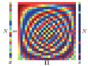
One of the primary goals in designing a WSN is the reduction of the energy consumption, to extend its lifetime without replacing or recharging the batteries of sensor nodes. The energy consumption of a sensor node mainly comes from three activities: sensing, data-processing and communication. Traditionally, the costs for processing and communication are assumed to dominate the overall energy consumption, while the cost for sensing is considered negligible. Therefore, a traditional WSN collects as much data as possible, that is subsequently compressed and transmitted with the lowest possible rate. In other words, it collects a vector of samples that is equal to the discretized physical field with some additive noise,
| (1) |
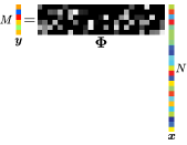
where is the identity matrix of size and represents the noise; see Figure 1a for an example.
If the energy consumed for sensing is comparable to that for communication and data processing, ignoring the energy cost of the former is sub-optimal. In fact, new sampling paradigms optimizing the overall energy consumption emerge and show that further reductions of the energy consumption are possible. The basic idea involves a reduction of the number of collected samples and a reconstruction of the missing data using algorithms exploiting the structure available in the measured data. The reduction of the collected samples is done by designing a sampling operator with , that it is used instead of the identity matrix as,
Note that is significantly shorter than and the reconstruction algorithm must estimate a significant amount of information from a limited amount of data. Therefore, regularization and constraints are added to the problem so that a stable solution can be obtained. Moreover, the reconstruction algorithm must be jointly designed with the sampling matrix to obtain a precise estimate of .
Pioneering work on sparse sampling considered compressive sensing (CS) as a reconstruction scheme. CS attempts to recover by solving a convex optimization problem, under the assumption that is sparse in a known dictionary . However, the solution is only approximate and it is exact if and satisfy certain requirements that are generally hard to check [4]. Initially, [8, 20, 13] proposed the use of a sampling matrix composed of random i.i.d. Gaussian entries. Note from Figure 1b that such has very few zero elements. Therefore, the number of sensing operations is not actually reduced because we need to know all the values of to compute . Moreover, if we adopt a distributed algorithm, a dense requires the sensor nodes to transmit their local samples to the other nodes, causing an excessive energy consumption for communications.
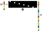
To overcome such limitations, [23, 14] proposed to use a sparse matrix which contains very few non-zero elements. More precisely, has generally only one non-zero element per row and the locations of such elements determine the spatio-temporal sampling pattern, see Figure 1c. However, the sampling patterns in these schemes are either fixed or randomly generated and thus not well adapted to the measured signal. Moreover, it is generally hard to guarantee the recovery of a faithful representation of , because the sparsity of dictionary usually changes over time and it may not satisfy the theoretical requirements of CS [5].
Since the statistics of are often unknown and varying over time, it may be advantageous to consider the decomposition
| (2) |
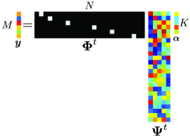
where is the time-varying model and is a low dimensional representation of with . While the ignorance and the non-stationarity of the model forces us to learn it from the samples collected in the past, it may give us the advantage of optimizing the sampling pattern according to . Note that is also time-varying as compared to the fixed pattern in Figure 1.
This new problem statement raises new challenges. While the model can be learnt from the incomplete measurements with some effort using an online version of the principal component analysis (PCA), the sampling scheduling problem is generally combinatorial and hard to optimize. In this paper, we propose to generalize FrameSense, an algorithm that generates a near-optimal sensor placement for inverse problems [16]. Instead of optimizing the sensor placement, we optimize the spatio-temporal sampling pattern of the WSN. The obtained sampling pattern is generally irregular, time-varying and optimized to gather the maximum amount of information. In particular, it simultaneously exploits the intra-node (temporal) and inter-node (spatial) correlation potentially present in the data. See Figure 2 for a graphical illustration of the low-dimensional model and of the irregular sampling patterns. Note that the proposed method deviates from the recent sparse sensing schemes [14, 23] because the sampling pattern is neither fixed nor random but dynamically adapted to the signal’s low-dimensional model.
It is worth mentioning that the proposed method imposes no on-sensor computation nor inter-node communication. Each sensor node simply collects measurements according to a designated sampling pattern and transmits the data to a common server. The server receives all the data from one or multiple sensor nodes and performs signal reconstruction. This is actually in accordance to the setup of distributed source coding [19], where no inter-node communication is used. Hence, the proposed algorithm provides an alternative solution to the distributed coding problem: the communication rate is reduced and the reconstruction error is bounded without using any inter-node communication.
The proposed algorithm is tested on different sets of real-word data, outperforming both the traditional sensing schemes and the state-of-the-art sparse sensing schemes, in terms of reconstruction quality of given a fixed amount of measurements. Given the aforementioned characteristics, we call the proposed method “Distributed Adaptive Sparse Sensing”, or DASS.
II Problem Formulation
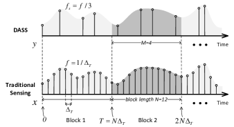
In this section, we first state the sampling scheduling problem for a WSN having just one sensor. At the end of the section, we generalize the problem statement to a WSN with multiple nodes. We consider a block-based sensing strategy, meaning that the WSN samples the field for a certain time and at the end we reconstruct the vector from the collected samples. Note that the block length is known and defined a-priori.
For each temporal block, the discrete physical field is composed of samples of ,
| (3) |
where indicates the sensor node location and is the sampling period. Note that determines the desired temporal resolution and its inverse is the sampling frequency, . The temporal duration of a block is , that is also the maximum delay this sensing scheme occurs—the larger , the longer the delay. See Figure 3 for a graphical representation of the physical field and its discrete version .
We denote the reconstructed physical field obtained from the WSN samples as . In a sparse sampling scenario, we aim at reconstructing from just a subset of elements of . More precisely, we measure elements out of , where . The set of indices denotes the indices of these samples and it is chosen adaptively according to the previous measurements. Note that the sampling pattern uniquely determines the sampling matrix :
It is important to underline that is time-varying and potentially changes at every block to adapt to the signal model . Figure 3 shows an example of sampling patterns where changes for each block.
We define to be the average sampling frequency of the sensor node111Note that it is an average frequency given the irregular and time-varying sampling pattern.. The subsampling rate is an important figure of merit for a sparse sampling algorithm—the lower the , the lower the energy consumed for sensing.
The measured signal is defined as
| (4) |
where represents the measurement noise, that is modeled as an additive white Gaussian noise (AWGN) with variance . Note that it is reasonable to model the noise phenomena as AWGN since the thermal effects [12] or/and quantization [22] are often the dominating terms222Other noise model may be of interest for specific sensors; for example the noise term of a Geiger counter is usually modeled as a Poisson process..
The target of DASS is to optimize the sampling pattern at the -th block according to such that we collect the minimum number of samples while still being able to recover precisely the original signal. Since we modeled the noise as a AWGN, we assess the quality of the recovered signal by using root-mean-square error (RMSE):
| desired number of samples in a block | number of measurements in a block, equals | ||
| temporal resolution of original signal | sampling frequency of original signal, equals | ||
| average sampling frequency of the sensor | subsampling rate | ||
| reconstructed signal | original signal | ||
| measured signal | measurement noise | ||
| sampling pattern of the -th block | sampling matrix of the -th block | ||
| mean of the signal | signal model of the -th block | ||
| low dimensional representation of | rows of selected by |
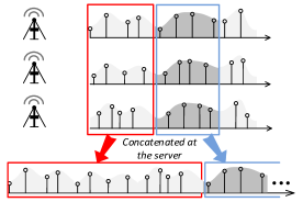
Multiple-node scenario: while the above problem statement focuses on a single-sensor scenario for simplicity of notation, it is simple to generalize the statement to a WSN with more than one sensor node. More precisely, we assume that the nodes are synchronized, so that we can concatenate all the measured blocks at different locations in a unique signal block , see Figure 4 for an example. The sparse sampling problem is generalized to a spatio-temporal domain meaning that we have to choose when and where we want to sample to collect the maximum amount of information.
III Building Blocks
The proposed method is graphically represented in Figure 5 and is based on the three building blocks described in this section:
-
1)
The desired signal is reconstructed using the collected measurements , the signal model and the estimated mean (Section III-A).
-
2)
The measurements are used to update the approximation model (Section III-B).
-
3)
The sampling pattern for the next temporal block is optimized according to and is transmitted back to the sensor node(s) (Section III-C).
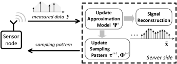
The overhead of DASS on the sensor node is minimal in practice. First, the sampling pattern has a sparse structure and hence it can be encoded efficiently with a few bytes per block. Therefore, the extra communication cost for receiving is minimal. Second, all the algorithmic complexity of DASS is at the server side, while the sensor nodes only need to sample and transmit the signal according to the sampling pattern received from the server. Therefore, the CPU and memory requirements of the sensor node are minimal.
In what follows, we analyze each block explaining the challenges and the proposed solution.
III-A Signal Approximation and Reconstruction
Due to the nature of most physical fields, a signal block is partially predictable by analyzing past data. In many cases, this predictability can be expressed by assuming that the signal belongs to a -dimensional linear subspace . Such a subspace approximates as
| (5) |
where is the approximated field, is the vector of the projection coefficients and is the mean of .
If the modeling subspace is well designed and is sufficiently large compared to the complexity of , the signal realization can be accurately expressed with just coefficients contained in . To find such a subspace, we analyze all the past signal realizations and estimate at the -th block the -dimensional subspace that minimizes the expected approximation error
This is a dimensionality reduction problem that can be solved by the well known technique of principal component analysis (PCA). It has an analytic solution but it requires the covariance matrix .
Unfortunately, in our scenario it is hard to estimate since we have access only to out of elements of . However, if the sampled elements are varying at each temporal block , we may collect enough information to have a sufficiently precise estimate of . We present a set of methods to estimate in Section III-B.
Note that the approximation through exploits the correlation among the elements of . The higher the correlation available in , the lower the dimensionality of the subspace , the number of parameters and the necessary measurements . Hence, one of the key aspects is the choice of the signal block length . In fact, it should be chosen such that the delay of the WSN respects the design specification while maximizing the correlation among the blocks. For example, if we consider a sensor measuring the outdoor light intensity, the signal itself naturally has diurnal patterns. If we choose a block length of one hour, the correlation between the signal block is usually weak. On the other hand, if we choose a block length of one day, the correlation is stronger due to the aforementioned patterns.
Once the approximation model is estimated, the task of recovering the signal amounts to estimating from the measurements when considering the approximated signal model
| (6) |
In general, we can recover by solving an Ordinary Least Square (OLS) problem:
| (7) |
which has the following analytic solution
| (8) |
Here is the Moore-Penrose pseudoinverse of that is defined for a generic matrix as .
The reconstruction algorithm is straightforward and is described in Algorithm 1. The following theorem states the necessary conditions to find a unique solution and provides an upper bound for the reconstruction error, that is going to be fundamental when optimizing the sampling pattern.
Theorem 1.
Consider a sensor network measuring a physical field as in (6) where the measurements are corrupted by an i.i.d. Gaussian noise with variance . If , is formed by orthonormal columns and , then can be uniquely determined using Algorithm 1. The reconstruction error is bounded by
| (9) |
where is the approximation error due to the signal model and are the eigenvalues of sorted in decreasing order.
Proof:
Since the Gaussian noise is independent from the approximation error, we can treat them independently. Moreover, it is sufficient to compute the error on the estimation of given the orthonormality of the columns of .
For the approximation error , we look at the worst case scenario with the following optimization problem
whose solution is proportional to the largest eigenvalue of . More precisely, it is possible to show that approximation noise is equal to the , where is the norm of the approximation error.
For the white noise, we consider a previous result given in [9] to conclude the proof. ∎
The upper-bound of the total error is a function of both the approximation error and measurement noise. The former term depends on the number of parameters : when , we have and it grows when we decrease . However, the rate at which the error increases depends on the spectrum of . In fact, if has elements that are highly correlated, a small could be sufficient to model with a small approximation error. The latter term can be controlled directly by optimizing the sampling pattern. More precisely, we cannot reduce but we can reduce the amplification due to the spectrum through an optimization of the sampling matrix .
Note that the part involving depends only on the smallest eigenvalue because we are not guaranteed that the approximation error spreads over all the eigenvectors of . In fact, the worst case scenario is represented by the approximation error being in the same direction of the eigenvector with the smallest eigenvalue and is consequently maximally amplified.
Compared to the methods based on CS, our approach based on a low-dimensional model and OLS has the following advantages: i) the solution is easy to compute and it requires a single matrix inversion, ii) it enables an analysis of the reconstruction error and a consequent optimization of the sampling pattern such that is minimized.
III-B Learning from Incomplete Data Over Time
In Section III-A, we have highlighted some challenges regarding the estimation of the covariance matrix — a fundamental step to determine the approximation model . Most of the challenges derive from the lack of a sufficiently large set of realizations of , that are needed to estimate . First, there is virtually no past data for a newly installed WSN. Second, is likely to vary over time. Third, a high ratio of data points () are not available for the estimation since we collect sparse measurements. Therefore, we need an on-line algorithm that estimates and adaptively updates the covariance matrix from incomplete data.
The main difficulty is the lack of complete realizations of . Two strategies are generally considered to overcome such a problem. The first one proposes to estimate from an interpolation using classic interpolation methods such as linear, polynomial or spline interpolation. The second strategy skips the estimation of and attempts to perform directly the principal component analysis with the data having missing entries, see [15].
In our experience, the second class of algorithms is less performant for our purposes. Therefore, we focus our attention on the interpolation methods. More precisely, we analyze two different methods that implement an adaptive learning and updating of the approximation model from the interpolated signal : Algorithm 2 and Algorithm 3.
Algorithm 2 uses a FIFO buffer to store the most recent blocks. Whenever a new block is added into the buffer, the oldest block in the buffer is excluded. As the approximation model is estimated according to the signal realizations in the buffer, this scheme is able to capture the variation of signal statistics over time.
Algorithm 3 adaptively updates the approximation model via a technique called incremental PCA [10]. It does not keep signal realizations in memory, instead, it stores the largest eigenvalues of , , for . This method requires significantly less memory ( versus ), and shows better performance when compared to Algorithm 2. Note that in both algorithms, the choice of depends on the variability of the signal statistics for each specific application. In practice, we can cross-validate this parameter to find a suitable value (e.g., ). We discuss and compare the performance of these two algorithms in the experimental results.
III-C Sampling Scheduling Algorithm
According to Theorem 1, minimizing the overall error is equivalent to finding the optimal sampling pattern that minimizes (9). In this paper, we assume that the model is sufficiently precise and the dimensions is large enough so that the term due to the white noise is dominant.
Therefore, we would like to find the sampling pattern that minimizes the following cost function,
| (10) |
where are the eigenvalues of , and Note that this optimization is equivalent to finding the rows of that forms the submatrix with the smallest . However, it has been already shown that such optimization is NP-hard [7] and has a complexity , which is prohibitively high in practice.
In this section, we investigate approximate solutions to the scheduling problem that can be implemented efficiently. These approximate solutions are usually hard to find because the cost function has many local minima that are arbitrarily far away from the global minimum. Therefore, proxies of are usually chosen as a cost function for the approximated algorithm with a twofold aim: (i) inducing an indirect minimization of and (ii) being efficiently optimized by standard techniques, as convex optimization or greedy algorithms.
In this paper, we extend our recent work [16] about optimal sensor placement to solve the sampling scheduling problem. In fact, if we define the linear inverse problem to be the estimation of from , then the sensor scheduling problem is equivalent to sensor placement. The algorithm [16] optimizes the sensor placement by a greedy minimization of the frame potential [6], that is defined as
| (11) |
where is the -th row of and contains the set of candidate locations for sensing. Under some mild solutions, we proved that such an algorithm is near-optimal w.r.t. the RMSE of the solution.
In this work, we propose a sampling scheduling algorithm based on an equivalent greedy “worst-out” procedure: as input we have the signal model and we initially consider the identity matrix of size as the sampling matrix . At each iteration, we remove the row of that maximizes (11). After iterations we are left with an optimized that has only elements different from zero and has near-optimal performance when reconstructing from the measurements . Note that if satisfies the conditions given in [16], the obtained sampling matrix stably recovers from the measurements .
Furthermore, since a uniform sampling schedule is a commonly-used strategy that yields good performance in real applications [23], we compare it with the result returned by the greedy algorithm and opt for the one with smaller reconstruction error. Note that this error is approximated by the bound provided by Theorem 1. A detailed description of the overall algorithm is given in Algorithm 4.
IV Comparisons with Baseline Methods
In this section, we briefly summarize the state-of-the-art methods for the sparse sensing problem. They will serve as the baseline for comparisons in Section V.
The first category of methods [14, 23] are based on compressive sensing (CS). With the notations introduced in Section II, is the unknown signal, contains the incomplete measurements, and is a sparse sampling matrix with only elements different from zero. We assume to be sparse w.r.t. a dictionary . More precisely, we have and has just a few coefficients different from zero, that is (see [3] for more details). By approximating the norm with the norm [4], the reconstruction method for the noiseless case is:
| (12) |
while the one for the noisy case is
| (13) |
where measures the energy of the noise. Problem (12) and (13) are both convex and can be solved [4] in polynomial time using various solvers, in general iterative or based on convex optimization. In both methods, we use uniform sampling as the sampling scheduler — .
The second category of baseline methods [14] are based on learning the -dimensional time-varying model and a reconstruction via OLS as in Algorithm 1. We use two sampling schedulers, namely, a uniform sampling, and a random sampling where is randomly selected with a uniform distribution.
Table II lists all the methods (including DASS) that are evaluated in the experiments. To have a fair comparison, in CS-based methods and in OLS-based methods are both learnt333The experimental results show that is the best choice for CS-based methods, while is a parameter which needs to be optimized for OLS-based methods, see Section V-A. by the incremental PCA described in Algorithm 3.
V Evaluations of DASS and Sparse Sensing Methods
In this section we evaluate the performance of DASS and compare it with the state-of-the-art sparse sensing methods. Besides the experiments on the single-node case, we also verify DASS in the multi-node case where nearby sensor nodes measure spatially correlated signals. We use two real-world meteorological datasets as the ground truth, namely Payerne and Valais:
-
•
Payerne is provided by MeteoSwiss [1]. This dataset contains 1500 days of continuous measurements for two physical quantities (temperature and solar radiation)444We denote by Payerne-temperature the dataset of temperature measurements. The notation is similar for solar radiation., which are suitable for studying long-term performance of DASS. As MeteoSwiss only deployed a few observation stations across the whole nation, we use Payerne for evaluating the single-node case.
-
•
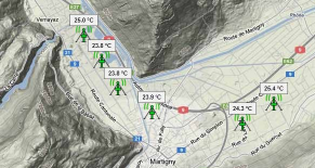
Valais is provided by a microclimate monitoring service provider [11]. A total of six stations are deployed in a mountain valley (Figure 6), covering an area of around . The deployments were started in March 2012 and collected 125 days of continuous temperature measurements. We use Valais for evaluating the multi-node case.
The two datasets are summarized in Table III. For both datasets, there are 144 uniformly sampled data points for each day. We choose the day as the length of each block, that is, .
One of the targets of this section is to evaluate DASS and compare it with other algorithms for different SNR regimes of the measurement. Since we cannot measure directly the real value of the physical field, we assume that Payerne and Valais represent the real value of the field . Then, we add white gaussian noise to simulate the effect of noisy measurements.
Note that the main merit figure considered in this section is the final reconstruction error under a fixed subsampling rate . Since all sparse sensing schemes directly transmit the sensing samples without further data compression, two schemes with the same have the same amount of energy consumed for sensing and communication555The processing costs of the considered sparse sensing methods are negligible., regardless of which sensing platform is used.
| Dataset name | Physical quantity | Number of nodes | Number of days |
|---|---|---|---|
| Payerne | temperature, solar radiation | 1 | 1500 |
| Valais | temperature | 6 | 125 |
V-A Components of DASS
In this section, we evaluate the key components of DASS, including the optimal choice of , the cost function in the sampling scheduling algorithm, and the performance of adaptive learning algorithms.
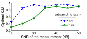
Optimal Choice of Dimension : As stated in Theorem 1, the overall reconstruction error is a function of both the approximation error and the cost function . Generally, decreases with and increases with , hence there is an optimal choice of for minimizing the overall error. The optimal depends on the data statistics, the subsampling rate, and the SNR of the measurement. By cross-validation, Figure 7 shows the optimal ratio for Payerne-temperature. We can see that DASS generally opts for a larger when the SNR of measurement increases.
Sampling Scheduling: The greedy algorithm proposed in Section III-C (Algorithm 4) finds an approximate solution of the sampling scheduling problem. By Theorem 1, determines the reconstruction error. Table IV shows the value of achieved by different sampling scheduling methods for different datasets. Note that a higher value indicates worse stability w.r.t. noise. We can see that the greedy algorithm achieves the best result for the two datasets. In particular, it is substantially better than uniform sampling for solar radiation data. For temperature data, since of the uniform sampling strategy is already near the lower bound666The lower bound of is if and only if is a basis., the greedy algorithm provides little improvement. In the next section, we demonstrate how these improvements translates into better reconstruction performance for DASS.
| uniform | random | Alg. 4 | |
|---|---|---|---|
| Temperature | 0.56 | 4.9 | 0.54 |
| Solar radiation | 4.5 | 1.8 | 0.97 |
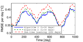
Learning Over Time: DASS is designed to learn the signal statistics from past data. In practical scenarios, a long backlog of data is usually infeasible and thus DASS should be designed to learn the model from scratch. We proposed Algorithm 2 and Algorithm 3 for this task. Figure 8 shows the learning curves of these two algorithms over three years of data. As a benchmark, we considered an offline method that learns the model from 600 days of past data and is represented by the red-dotted curve.
Note how Algorithm 2 and Algorithm 3 capture the signal statistics precisely. In particular, it is interesting to note that even if they use less data—the last 30 days—they are generally better than the offline method that considers 600 days of data. This phenomenon is due to the non-stationarity of the signal model that is captured only by adaptive on-line algorithms. Moreover, it is also clear that Algorithm 3 with incremental PCA performs better than the buffer-based Algorithm 2.
In the following experiments, we will only consider Algorithm 3 due to its better performance and lower memory requirements.
V-B DASS versus Baseline Methods
Here, we compare DASS with the baseline methods introduced in Table II, namely, CS, CSN, OLS-random, and OLS-uniform.
Known Noise Level: For DASS, we need to choose the optimal according to the cross-validation studied in Figure 7. Hence, we need to know the SNR of the measurement. A similar parameter tuning is necessary for CSN, where in Problem (13) represents the noise level. Therefore, whenever we consider the case of noisy measurements, an estimate of the SNR of the measurement is necessary to avoid degradations of the reconstruction quality.
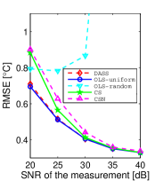
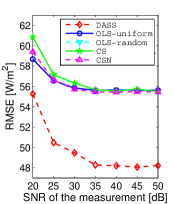
In the first experiment, we assume that the estimation of the SNR is exact. Figure 9 shows the comparison results of DASS, OLS-uniform, OLS-random, CS and CSN, for both temperature and solar radiation data. First, note that OLS-uniform generally performs better than the two CS-based schemes, especially in low SNR regime. In high SNR regime (dB), OLS-uniform, CS and CSN tend to perform the same. Second, the bad performance of OLS-random indicates that random sampling is not a valid sampling strategy for neither temperature nor solar radiation signals. Third, while DASS and OLS-uniform performs almost equivalently for temperature data, we can note that DASS is substantially better for solar radiation data. This fact is in accordance with the analysis of given in Table IV: if due to uniform sampling is large, then the sampling scheduling algorithm of DASS (Algorithm 4) significantly improves the effectiveness of sensing while preserving the average sampling rate.
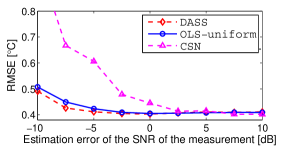
Error in Noise Estimation: In practice, the estimation of the noise level might be not exact. Here, we study the performance deviation of the considered algorithms when there is an error in such estimates. More precisely, we fix all the parameters and we vary the estimation error of the SNR and then measure the performance of the algorithms in terms of RMSE.
Figure 10 shows the reconstruction error with respect to the estimation error of SNR, whereas the true SNR is 30dB. We can see that DASS performs the best, and generally DASS and OLS-uniform are both stable w.r.t. errors in the SNR estimation. However, the performance of CSN degrades severely when the SNR is underestimated.
According to results given in Figure 9 and Figure 10, DASS is both more accurate and robust when compared to the state-of-the-art sparse sensing methods.
V-C DASS on Multiple Sensor Nodes
As discussed in Section II, the concept of DASS can be extended to multiple sensor nodes by concatenating the collected samples in a single vector and using the same strategy as for the single-node case.
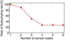
Merging the data of all the spatial nodes possibly augments the correlation; DASS may exploits such correlation to reduce the sampling rate. In fact, if all the measurements collected by the sensors are linearly independent then DASS generates the same sampling scheduling that would have been optimized for each sensor individually. However, if there exists some correlation between the different sensor nodes, then DASS jointly optimizes the sensor scheduling so that the total average sampling rate is reduced.
We denote by Joint DASS the scheme that jointly reconstructs the signals of the WSN (Figure 4), and Independent DASS the scheme that independently reconstructs the signals of each node. Note that in both schemes, sensor nodes are operating in a purely distributed manner; the difference is that Joint DASS aggregates the sensed data of all nodes and jointly processes them.
Figure 11 shows the ratio between the subsampling rates of Joint DASS and Independent DASS, using the data-set Valais. We can see that as the number of sensor nodes increases, the required sampling rate of Joint DASS also gradually decreases. In particular, with 4 nodes we can reduce the number of samples by 70% with Joint DASS. Therefore, exploiting the spatial correlation further enhances the energy reduction of DASS. On the other hand, the benefit flatten out when we consider 5 or more sensor nodes. The intuition behind this phenomenon is that the last two sensor nodes are far apart from the others and there is no more correlation to exploit, see the rightmost two nodes in Figure 6.
V-D Blocks with Weaker Correlation
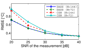
In real applications, the block length must be chosen such that the delay of the WSN respects the design specification while the correlation between blocks is maximized. In all experiments above, is chosen so that one block represents one day, which intuitively fits signals with strong diurnal cycles, such as temperature signals. In practice, it is essential to evaluate how DASS performs with a sub-optimal . In this section, we use the same dataset Payerne-temperature, but splitting one day into two blocks. This means that we transmit and reconstruct signals two times per day and hence the correlation between the different temporal blocks is smaller. Figure 12 compares DASS and CSN with two possible block length: a full day—— and half a day—. We can note that the performance of DASS is only slightly affected by the smaller block length, while CSN is considerably affected in the low SNR regime.
VI Energy Saving over Traditional Data Collection Schemes
In Section V, we have shown that DASS achieves better performance w.r.t. the state-of-the-art sparse sensing schemes. In this section, we study the overall energy saving of DASS w.r.t. the traditional data collection schemes [17, 24]. The energy saving is particularly significant on platforms where the energy consumed for sensing is more pronounced. This is intuitive since DASS can substantially reduce the number of sensing samples. Nevertheless, our analysis shows that this saving is also noticeable on platforms with small sensing cost, e.g. a Tmote-sky node [21].
The traditional data collection schemes typically sample the physical field at a high frequency as in (1) and then compress the samples to reduce the communication rate, see Figure 13a. In contrast, DASS collects measurements using an optimized sampling pattern and a reduced average sensing frequency , where . Then, each sensor node transmits the raw data points without any compression, see Figure 13b. In both traditional schemes and DASS, we aim at precisely reconstructing the signal .
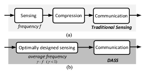
It is clear that DASS reduces the energy consumption for the sensing operations over the traditional scheme. However, DASS may not necessarily consume less communication energy, since the compression ratio 777 equals uncompressed size / compressed size. used in traditional sensing is generally better than . In fact, existing data compression schemes can achieve a compression ratio of for lossless coding [17], and for lossy coding [24], while a typical value of used in DASS is . Hence, there is a tradeoff between the energy saved on sensing and communications.
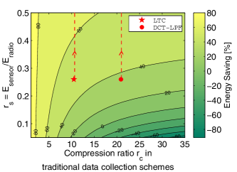
Such tradeoff between the different energy consumption depends on platform-specific parameters. In particular, we denote the energy consumption for collecting and transmitting one sample as and , respectively. An interesting figure is the ratio between the two energy values, that we denote as . Intuitively, the larger , the larger the energy savings obtained by DASS. For the traditional data collection schemes, we assume that the compression step has a negligible energy cost. For DASS we use a subsampling rate of , which means that 10% of the original signal is sampled and transmitted.
Under these assumptions, we can quantitatively analyze the relative energy savings of DASS w.r.t. the traditional sensing as a 2-D function of the platform parameter and the compression ratio achieved by the compression stage of the traditional scheme. Such function representing the energy saving is plotted in Figure 14. We see that there is a line, indicated by the zero value, that defines where DASS is more energy-efficient than the traditional schemes. Above the line, a WSN consumes less energy if it uses DASS and vice versa. Note that DASS is only less efficient in the scenarios where the compression ratio is very high and the platform parameter is very low.
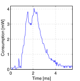
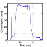
We also looked at the energy savings for a plausible real world scenario. More precisely, we consider Tmote-sky, a low-power sensing platform widely used in WSNs [21]; it has a photodiode sensor that measures the light intensity of the surroundings and can communication with others through short-range radio. We measured the two energy consumptions and of Tmote-sky in a set of experiments, and an example of the results is given in Figure 15. In particular, the experiments indicate that . To evaluate the energy consumption of a traditional scheme, we need to choose a specific compression algorithm and measure the achieved . Zordan et al. [24] have recently compared various lossy compression algorithms and showed that DCT-LPF [24] achieves the best performance in terms of compression ratio. However, it is also a complex algorithm and may have a significant energy consumption on a resource-limited platform such as Tmote-sky. Therefore, we also consider a lightweight algorithm, LTC [18], that achieves the lowest energy consumption on WSN nodes if the energy cost for compression is considered.
Here, we ignore the energy cost of compression and we compare both algorithms with DASS. Note that, if we consider computational energy cost, the benefit of DASS will be even larger since it requires minimal on-board computation. We implement and evaluate the two algorithms on the dataset Payerne-temperature, and record the corresponding compression ratio when their reconstruction errors are the same as those achieved by DASS.
The “star” and “circle” markers in Figure 14 show the energy savings of DASS over a Tmote-sky that compresses the data with LTC and DCT-LPF, respectively. The energy savings for the two cases are equal to 50% and 35% and go up to 60% if increases due to a higher energy cost for sensing, as denoted by the dashed lines in Figure 14. This scenario could be realistic for many WSNs, in particular those using sensor belonging to the following two classes:
-
•
Sensors with high energy consumption: for example an air pollution sensors consume mW instead of the 3 mW of a Tmote-sky’s light sensor.
-
•
Sensors with long sampling time: for example the anemometer, a sensor that measures wind’s direction and strength, requires seconds of continuous measurement per sample instead of the 4 ms of the Tmote-sky’s light sensor.
VII Conclusions
In this paper, we proposed DASS, a novel approach for sparse sampling that optimizes sparse sampling patterns for precisely recovering spatio-temporal physical fields. DASS is based on three main blocks. First, it adaptively learns the signal statistics from past data. Second, it dynamically adjusts the sampling pattern according to the time–varying signal statistics. Third, it recovers the signal from the limited amount of collected samples and according to the learnt signal statistics.
We demonstrated the effectiveness of DASS through extensive experiments using two real-world meteorological datasets. The results show significant improvements over the state-of-the-art methods. These improvements are more pronounced in the presence of significant spatial and/or temporal correlation in the sampled data by WSN.
We evaluated DASS on static WSNs; however, DASS is flexible and can be applied to other sensing scenarios such as mobile WSNs. For instance, sensors are installed on top of buses for collecting various environmental data along their trajectories [2]. The collected samples show strong correlation due to the fixed route periodically taken by the buses. In future work, we will analyze the advantages of an optimized sensing schedule in such cases, where the constraint is not the energy consumption but the relatively slow speed of sampling of certain pollution sensors.
References
- [1] MeteoSwiss: the Federal Office of Meteorology and Climatology of Switzerland. http://www.meteoswiss.admin.ch.
- [2] K. Aberer, S. Sathe, D. Chakraborty, A. Martinoli, G. Barrenetxea, B. Faltings, and L. Thiele. Opensense: open community driven sensing of environment. In Proc. IWGS, pages 39–42. ACM, 2010.
- [3] E. Candès. Compressive sampling. In Proceedings of the International Congress of Mathematicians: invited lectures, pages 1433–1452, 2006.
- [4] E. Candes, J. Romberg, and T. Tao. Stable signal recovery from incomplete and inaccurate measurements. Communications on pure and applied mathematics, 59(8):1207–1223, 2006.
- [5] E. J. Candès, E. J. Candès, M. B. Wakin, and M. B. Wakin. An Introduction To Compressive Sampling. IEEE Signal Process. Mag., 25(2):21–30, 2008.
- [6] P. G. Casazza, M. Fickus, J. Kovačević, M. Leon, and J. Tremain. A physical interpretation of tight frames. Harmonic analysis and applications, pages 51–76, 2006.
- [7] A. Das and D. Kempe. Algorithms for Subset Selection in Linear Regression. In Proceedings of the 40th annual ACM symposium on Theory of computing, pages 45–54. ACM, 2008.
- [8] M. F. Duarte, M. B. Wakin, D. Baron, and R. G. Baraniuk. Universal distributed sensing via random projections. In Proc. IPSN, pages 177–185, Nashville, TN, Apr. 2006.
- [9] M. Fickus, M. Fickus, D. G. Mixon, D. G. Mixon, M. J. Poteet, and M. J. Poteet. Frame completions for optimally robust reconstruction. arXiv, July 2011.
- [10] P. M. Hall, D. Marshall, and R. R. Martin. Incremental eigenanalysis for classification. In Proc. BMVC, pages 286–295, 1998.
- [11] F. Ingelrest, G. Barrenetxea, G. Schaefer, M. Vetterli, O. Couach, and M. Parlange. Sensorscope: Application-specific sensor network for environmental monitoring. ToSN, 6, March 2010.
- [12] J. Johnson. Thermal agitation of electricity in conductors. Physical Review, 32(1):97, 1928.
- [13] C. Luo, F. Wu, J. Sun, and C. W. Chen. Compressive data gathering for large-scale wireless sensor networks. In Proc. Mobicom, pages 145–156. ACM, 2009.
- [14] G. Quer, R. Masiero, G. Pillonetto, M. Rossi, and M. Zorzi. Sensing, compression, and recovery for wsns: Sparse signal modeling and monitoring framework. IEEE Trans. Wireless Commun., 2012.
- [15] T. Raiko, A. Ilin, and J. Karhunen. Principal component analysis for sparse high-dimensional data. In Proc. ICONIP, pages 566–575. Springer, 2008.
- [16] J. Ranieri, A. Chebira, and M. Vetterli. Near-Optimal Sensor Placement for Linear Inverse Problems. submitted, IEEE Trans. Signal Process., pages 1–11, June 2013.
- [17] C. M. Sadler and M. Martonosi. Data compression algorithms for energy-constrained devices in delay tolerant networks. In Proc. SenSys. ACM, 2006.
- [18] T. Schoellhammer, B. Greenstein, E. Osterweil, M. Wimbrow, and D. Estrin. Lightweight temporal compression of microclimate datasets. In Proc. 29th Annual IEEE International Conference on Local Computer Networks, pages 516–524, 2004.
- [19] K. Viswanatha, S. Ramaswamy, A. Saxena, and K. Rose. Error-resilient and complexity-constrained distributed coding for large scale sensor networks. In Proc. IPSN, pages 293–304. ACM, 2012.
- [20] W. Wang, M. Garofalakis, and K. Ramchandran. Distributed sparse random projections for refinable approximation. In Proc. IPSN, pages 331–339. IEEE, 2007.
- [21] G. Werner-Allen, K. Lorincz, M. Ruiz, O. Marcillo, J. Johnson, J. Lees, and M. Welsh. Deploying a wireless sensor network on an active volcano. IEEE Internet Comput., 10, 2006.
- [22] B. Widrow and I. Kollár. Quantization noise. Cambridge University Press, 2008.
- [23] X. Wu and M. Liu. In-situ soil moisture sensing: measurement scheduling and estimation using compressive sensing. In Proc. IPSN. ACM, 2012.
- [24] D. Zordan, B. Martinez, I. Vilajosana, and M. Rossi. To compress or not to compress: Processing vs transmission tradeoffs for energy constrained sensor networking. arXiv preprint arXiv:1206.2129, 2012.