Nuclear constraints on the equation of state and rotating neutron stars

Abstract

In this contribution nuclear constraints on the equation of state for a neutron star are discussed. A combined fit to nuclear masses and charge radii leads to improved values for the symmetry energy and its derivative at nuclear saturation density, $S_{\rm{v}}=31$ MeV and $L=68\pm 8$ MeV. As an application the sensitivity of some properties of rotating supramassive neutron stars on the EoS is discussed.

1 Nuclear Constraints on the Equation of State

Despite numerous efforts to tighten the nuclear constraints on the EoS there remains considerable uncertainty. The spreading in the pressure at nuclear saturation density as summarized by Lattimer [1] a decade ago was roughly a factor six; results of present day mean field calculations vary by about a factor four [2]. Therefore it remains a challenge to try to improve the situation.
The pressure as a function of density is given by $P(\rho)=\rho d\epsilon/d\rho-\epsilon(\rho).$
In neighborhood of saturation density $\rho_{s}$, with $u=\rho/\rho_{s}$ and $x$ proton fraction one has

$$\epsilon(u,x)=B+K/18(u-1)^{2}+S_{A}(u)(1-2x)^{2}+..,$$ (1)

where $K$ the compressibility and $S_{A}$ the symmetry energy (SE). Hence the pressure near $\rho_{s}$ is

$$P(\rho\sim\rho_{\rm{s}})\sim u^{2}\rho_{\rm{s}}[\frac{K}{9}(u-1)+\frac{dS_{A}}{du}(1-2x)^{2}+..].$$ (2)

In practice the leading contribution comes from the last term, the derivative of the SE; the latter is usually parameterized in the liquid drop model (LDM) as

$$S_{A}=\frac{(N-Z)^{2}}{A}\frac{S_{\rm{v}}}{1+yA^{-1/3}},$$ (3)

where $S_{\rm{v}},\ S_{\rm{s}}$ denote the volume and surface SE, and $y=S_{\rm{v}}/S_{\rm{s}}$.
The quantity of interest for the EoS, the derivative $L=3\rho_{s}dS/d\rho|_{s}$, can in good approximation [1] be related to $S_{\rm{v}}$ and $y$: ${{y}}\sim 0.646+S_{\rm{v}}/98$MeV$+0.436L/S_{\rm{v}}+0.087(L/S_{\rm{v}})^{2}$.
In practice the values of $S_{\rm{v}},y$ when fitted to masses using the LDM appear to be strongly correlated [3], and the same is true for $L$, $S_{\rm{v}}$ (see the 1-$\sigma$ confidence ellips in fig. 1), and a similar correlation is found in microscopic (mean field) models.

Figure 1: Constraints on $L\ vs\ S_{\rm{v}}$, the filled ellipsoid corresponds to the constraint from fitting nuclear masses, from [1].

However, one can improve the situation sketched above in several ways. As a first step one may consider differentials of masses with respect to $N-Z$ (rather than a global fit), which allows one to fit the parameters in $\frac{S_{\rm{v}}}{1+yA^{-1/3}}$ in isolation of other terms [4, 5].
By plotting $1/S$ vs $A^{-1/3}$ (see fig. 2) one obtains the value of $1/S_{\rm{v}}$ from the crossing of the fit line with y-axis ($A=\infty$) and the slope $y=2.6\pm 0.8$. From the figure the correlation between slope and $S_{\rm{v}}$ is evident.
As a second step an appreciable increase in the accuracy can be achieved by including shell corrections [4] shown in the right part of the figure.

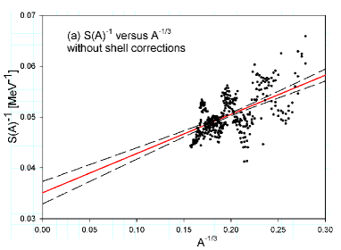
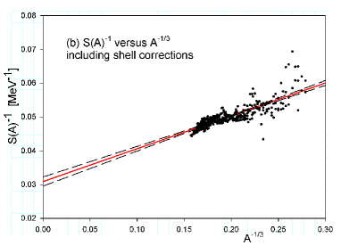
Figure 2: SE vs $A^{-1/3}$ without (left) and with (right) shell corrections, from [4].

In passing we note that in ref. [6] a quite accurate result for $S_{\rm{v}},\ S_{\rm{s}}$ is reported by using double differences of masses. However, their results are obtained for a parametrization of the SE different from eq. (3), and moreover depend on the choice of the Wigner energy.
As a final step one can improve the situation further by using information from charge radii, which mainly depends only on the ratio $y$. (In fig. 1 this is indicated by the band labeled “skins of Sn”, but we consider the result of this particular analysis rather model dependent).
In the spirit of the LDM and distinguishing proton and neutron radii we decompose [4]

$$R_{\rm{p}}(N,Z)=R_{0}(N,Z)+\frac{N}{A}R_{\rm{np}}(N,Z)+\delta R_{\rm C}(N,Z),$$ (4)

where the isoscalar term $R_{0}=(NR_{\rm n}+ZR_{\rm p})/A\sim r_{0}A^{1/3},$ and the isovector term (essentially the neutron skin)

$$R_{\rm{np}}=R_{\rm n}-R_{\rm p}=\frac{2r_{0}}{3}\frac{N-Z}{A}\frac{1}{1+A^{1/3}/y},$$ (5)

and $R_{C}$ the Coulomb contribution [3]. The point is that $R_{\rm{np}}$ depends only on $y=S_{\rm{v}}/S_{\rm{s}}$ (apart from the Coulomb contribution).
To determine $y$ from data one can envision the following options
(i) measure the neutron skin using parity violating electron scattering (PREX). However, the first experiment [7] on ²⁰⁸Pb yielded a rather large error $R_{\rm{np}}\sim 0.33\pm 0.17$ fm.
(as a side remark: atomic parity violation, in progress, appears a promising alternative tool, with a possible precision of about 1% in the skin in Ra isotopes),
(ii) fit to observed charge radii using the expression (4). (As an alternative one may consider fitting differences like isobar shifts, $R_{\rm p}(N,Z)-R_{\rm p}(N-i,Z+i)$; the latter are independent of $R_{0}$, but in general have larger experimental uncertainties.)
The values for $S_{\rm{v}}$ and $y$ from a combined fit of masses and radii are given in table 1, which are compared to some other results from fits and microscopic approaches.

Table 1: Results for the parameters $S_{\rm{v}},\ y$ and $L$ obtained from fits and microscopic approaches

$S_{\rm{v}}$(MeV)	$y$	$L$(MeV)	$R_{\rm{np}}$(208Pb) (fm)	ref	model
		fit to masses
$32.5\pm 0.5$	1.98	$70\pm 15$		[8]	FRLDM
$32.1\pm 0.3$	1.9			[6]	double diff
31.1	$2.31\pm 0.38$	$66\pm 13$		[10]	LDM
32	3.0	94		[5]	analysis IAS
31	$2.5\pm 0.4$	$80\pm 15$		[4]	LDM+shell corr
30.5	$2.35\pm 0.20$	$68\pm 8$	$0.185\pm 0.015$	present	masses+ charge radii
		Microscopic	approaches
30		$58\pm 15$		[9]	Skyrme+skin Sn isotopes
$32\pm 1.5$		$45\pm 15$		[11]	QMC
$31\pm 1$	$1.85\pm 0.25$	$46\pm 10$		[13]	EFT
$31\pm 1$		$64\pm 8$	$0.195\pm 0.02$	[12]	EDF

Note that phenomenology seems to favor larger $L$ values than most microscopic models; this trend is not understood yet.

2 Rotating supramassive neutron stars and the EoS

Several energetic observations can be associated with formation of neutron stars (NS) or black holes (BH), supernovae, gamma ray bursts (GRB). Some short GRB’s ($\sim$1s) have been attributed to NS mergers.
Recently the observation [14] of bright radio pulses was reported, with radio flux $\sim$ Jy at GHz frequencies and $\Delta T\leq 1$ms, which do not repeat, while no $\gamma$- or x-rays were observed.
Falcke and Rezzolla [15] proposed the following interpretation: a supramassive rotating NS (i.e., a NS with a mass larger than the maximum mass of a static NS, e.g. created by accretion in binary system) slows down due to magnetic braking, and at critical point collapses into Kerr BH (see fig. 3).

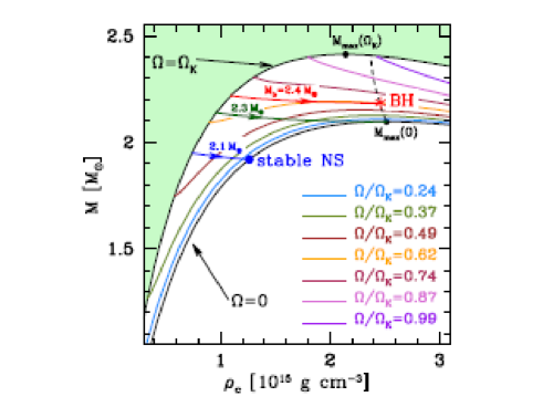
Figure 3: Gravitational mass vs central density for various ratios $f=\Omega/\Omega_{K}$, where $\Omega_{K}$ is taken as the critical $\Omega$ belonging to star with maximum mass; arrows represent tracks of NS’s slowing down due to magnetic braking, from [15].

The created event horizon will hide star’s surface, hence only emission from the detached magnetosphere can be observed; the estimated timescale (freefall) $\tau\sim 0.04R_{10}^{3/2}M_{2}^{-1/2}$ ms appears to be consistent with the observation.
For a non-rotating star the mass vs radius relation (given the EoS) is obtained by solving the TOV equation; a rotating star requires a more general approach to general relativity.

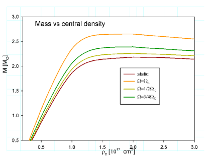
Figure 4: Gravitional mass vs radius (left) and vs central density (right) for various $\Omega$. In the left panel the broken line denotes the lower limit on the mass of a static star from eq. (7).

The scenario proposed in ref. [15] seems not unrealistic but some questions remain. For example the authors took a very simple representation for the EoS: a single polytrope $P={{K}}\rho^{\gamma}$ with $\gamma=2$ and $K$ adjusted such that $M(0)_{\rm{max}}=2.1M_{\odot}$.
Naturally one may ask how large is the sensitivity to EoS? To investigate this we took a 3-polytrope EoS , $P(\epsilon)=K_{i}\epsilon^{\Gamma_{i}}$. It fits $P(\rho_{s})$ and has the proper low-density behavior; specifically, $\Gamma_{1}=1.5$ for $\epsilon<67$ MeV/fm³, $\Gamma_{2}=2.68,$ for $67<\epsilon<650$, and $\Gamma_{3}=1.41$ for $\epsilon>650$. The $K_{i}$ values are fixed by continuity of the pressure $P$ and the normalization $P(\epsilon=650)=180$ MeV/fm³. It yields $M_{\rm{max}}=2.2M_{\odot}$.
Using the rns code [17] the mass as a function of the equatorial radius or the central density, and the critical frequency (the Keppler or mass shedding limit) have been computed, see fig. 4.
Qualitatively the main features of fig. 3 are confirmed, i.e., $M(\Omega_{K})$ increases by 20$\%,$   $R(\Omega_{K})$ increases by 50%. However, $\Omega_{K}$ itself turns out to be more sensitive to the EoS [18, 16].
Finally we point out that an observation of a high rotation frequency of a pulsar can lead to a constraint on the mass-radius diagram. Namely for a Newtonian uniformly rotating rigid star with mass $M$ and radius $R$ one has

$$\tau_{\rm{min}}=2\pi\sqrt{\frac{R^{3}}{GM}}=0.545\left(\frac{M_{\odot}}{M}\right)^{1/2}\left(\frac{R}{\rm{10km}}\right)^{3/2}\rm{ms}.$$ (6)

Using general relativity a similar empirical relation (valid for $M<0.9M_{\rm{max}}(0)$ with a weak dependence on the EoS) has been derived [18] ($M,R$ refer to the static star)

$$\tau_{\rm{min}}=C\ (M_{\odot}/M)^{1/2}(R/{\rm{10km}})^{3/2}\rm{ms},$$ (7)

where $C\sim 0.92\pm 0.04$; with our EoS we find $C=0.90$. At present, the fastest rotating pulsar has $\nu_{obs}$ = 716 Hz. Obviously, the Keplerian frequency of any neutron star must satisfy $\nu_{K}\geq\nu_{\rm{obs}}.$ This inequality constraints a region on the $M\ vs\ R$ diagram as shown in the left panel of fig. 4.

References

References

- [1] Lattimer J M (2012) Ann. Rev. Nucl. Part. Sci. 62 485
- [2] Steiner A and Gandolfi S (2012) Phys. Rev. Lett. 108 081102
- [3] Danielewicz P (2003) Nucl. Phys. A727 203
- [4] Dieperink A and van Isacker P (2009) Eur. J. Phys. A32 11
- [5] Danielewicz P and Lee J (2009) Int. J. Mod. Phys. E18 892
- [6] Jiang H et al. (2012) Phys. Rev. C85 024301
- [7] Abrahamyan S et al. (2012) Phys. Rev. Lett. 108 112502
- [8] Möller P et al. (2012) Phys. Rev. Lett. 108 052501
- [9] Chen L W et al. (2010) Phys. Rev. C82 024321
- [10] Liu M et al. (2010) Phys. Rev. 82 064306
- [11] Gandolfi S et al. (2012) Phys. Rev. C85 032801(R)
- [12] Agrawal B K et al. (2013) arXiv: nucl-th/1305.5336
- [13] Hebeler K et al. (2010) Phys. Rev. Lett. 105 160102
- [14] Thornton D et al. (2013) Science 341 53
- [15] Falcke H and Rezzolla L (2013) arXiv: astro-ph/1307.1409
- [16] Lo K-W and Lin L-M (2011) Astrophys. J. 728 12
- [17] Stergioulas N and Friedman J L (1995) Astrophys. J. 444 306
- [18] Haensel P et al. (2009) A.&A. 502 605