A Principled Infotheoretic $\phi$-like Measure

Abstract

Integrated information theory [1, 2, 3] is a mathematical, quantifiable theory of conscious experience. The linchpin of this theory, the $\phi$ measure, quantifies a system’s irreducibility to disjoint parts. Purely as a measure of irreducibility, we pinpoint three concerns about $\phi$ and propose a revised measure, $\psi$, which addresses them. Our measure $\psi$ is rigorously grounded in Partial Information Decomposition and is faster to compute than $\phi$.

1 Introduction

The measure of integrated information, $\phi$, is an attempt to a quantify a neural network’s magnitude of conscious experience. It has a long history [4, 1, 5], and at least three different measures have been called $\phi$. Conceptually, the $\phi$ measure aims to quantify a system’s “functional irreducibility to disjoint parts”. Although innovative, the $\phi$ measure from [1] has some peculiarities. Using Partial Information Decomposition (PID), we derive a principled info-theoretic measure of irreducibility to disjoint parts[6]; our PID-derived measure, $\psi$, has numerous desirable properties over the $\phi$ from [1].

We aim for $\psi$ to be a principled, well-behaved $\phi$-like measure that resides purely within Shannon information theory. We compare $\psi$ to the older $\phi$ measure from [1] because it is the most recent purely information-theoretic $\phi$. We recognize that the most recent version of $\phi$[5] knowingly and purposely sits outside standard information theory.^,

2 Preliminaries

We use the following notation throughout.

$n$:

the number of indivisible elements in network $X$. $n\geq 2$.

$\mathbf{P}$:

a partition of the $n$ indivisible nodes clustered into $m$ parts. Each part has at least one node and each partition has at least two parts, so $2\leq m\leq n$.

$X^{\mathbf{P}}_{i}$:

a random variable representing a part $i$ at time=$0$. $1\leq i\leq m$.

$Y^{\mathbf{P}}_{i}$:

a random variable representing part $i$ after $t$ updates. $1\leq i\leq m$.

$X$:

a random variable representing the entire network at time=$0$. $X\equiv X^{\mathbf{P}}_{1}\cdots X^{\mathbf{P}}_{m}$.

$Y$:

a random variable representing the entire network after $t$ applications of the neural network’s update rule. $Y\equiv Y^{\mathbf{P}}_{1}\cdots Y^{\mathbf{P}}_{m}$.

$y$:

a single state of the random variable $Y$.

$\mathbf{X}$:

The set of the $n$ indivisible elements at time=$0$.

For readers accustom to the notation in [1] the translation is: $X\equiv X_{0}$, $\ Y\equiv X_{1}$, $\ X^{\mathbf{P}}_{i}\equiv M_{0}^{i}$, and $Y^{\mathbf{P}}_{i}\equiv M_{1}^{i}$.

For pedagogical purposes we confine this paper to deterministic neural networks. Therefore all remaining entropy at time $t$ conveys information about the past, i.e., $\operatornamewithlimits{I}\!\left(X\!\mathrel{\mathop{\mathchar 58\relax}}\!Y\right)=\operatornamewithlimits{H}\!\left(Y\right)$ and $\operatornamewithlimits{I}\!\left(X\!\mathrel{\mathop{\mathchar 58\relax}}\!Y^{\mathbf{P}}_{i}\right)=\operatornamewithlimits{H}\!\left(Y^{\mathbf{P}}_{i}\right)$ where $\operatornamewithlimits{I}\!\left(\bullet\!\mathrel{\mathop{\mathchar 58\relax}}\!\bullet\right)$ is the mutual information and $\operatornamewithlimits{H}\!\left(\bullet\right)$ is the Shannon entropy[7]. Our model generalizes to probabilistic units with any finite number of discrete—but not continuous—states[8]. All calculations are in bits.

2.1 Model Assumptions

1. The $\phi$ measure is a state-dependent measure. Meaning that every output state $y\in Y$ has its own $\phi$ value. To simplify cross-system comparisons, some researchers[8] prefer to consider only the averaged $\phi$, denoted $\langle\phi\rangle$. Here we adhere to the original theoretical state-dependent formulation. However, when comparing large numbers of networks we use $\langle\phi\rangle$ for convenience.

2. The $\phi$ measure aims to quantify “information intrinsic to the system”. This is often thought to be synonymous with causation, but it’s not entirely clear. But for this reason, in [1] all random variables at time=$0$, i.e., $X$ and $X^{\mathbf{P}}_{1},\ldots,X^{\mathbf{P}}_{m}$ are forced to follow an independent discrete uniform distribution. There are actually several plausible choices for the distribution on $X$ (see Appendix E). But for easier comparison to [1], here we also take $X$ to be an independent discrete uniform distribution. This means that $\forall i\not=j\ \ \operatornamewithlimits{I}\!\left(X^{\mathbf{P}}_{i}\!\mathrel{\mathop{\mathchar 58\relax}}\!X^{\mathbf{P}}_{j}\right)=0$ and $\operatornamewithlimits{H}\!\left(X\right)=\log_{2}\left|X\right|$, $\operatornamewithlimits{H}\!\left(X^{\mathbf{P}}_{i}\right)=\log_{2}\left|X^{\mathbf{P}}_{i}\right|$ where $|\bullet|$ is the number of states in the random variable.

3. We set $t=1$, meaning we compute these informational measures for a system undergoing a single update from time=$0$ to time=$1$. This has no impact on generality (see Appendix D). To analyze real biological networks one would sweep $t$ over all reasonable timescales choosing the $t$ that maximizes the complexity metric.

3 How $\phi$ Works

The $\phi$ measure has four steps and proceeds as follows.

1. For a given state $y\in Y$, [1] first defines the state’s effective information quantifying the total magnitude of information the state $y$ conveys about $X$, the r.v. representing a maximally ignorant past. This turns out to be identical to [9]’s “specific-surprise”, $\operatornamewithlimits{I}\!\left(X\!\mathrel{\mathop{\mathchar 58\relax}}\!y\right)$,

   $${\tt ei}(X\rightarrow y)=\operatornamewithlimits{I}\!\left(X\!\mathrel{\mathop{\mathchar 58\relax}}\!y\right)=\operatorname{D_{KL}}\!\left[\Pr\!\left(X|y\right)\middle\|\,\Pr\!\left(X\right)\right]\;.$$ (1)

   Given $X$ follows a discrete uniform distribution (assumption (B)), ${\tt ei}(X\rightarrow y)$ simplifies to,

   $$\begin{split}{\tt ei}(X\rightarrow y)&=\operatornamewithlimits{H}\!\left(X\right)-\operatornamewithlimits{H}\!\left(X|y\right)\\ &=\operatornamewithlimits{H}\!\left(X\right)-\sum_{x\in X}\Pr\!\left(x|y\right)\log_{2}\frac{1}{\Pr\!\left(x|y\right)}\;;\end{split}$$ (2)

   in the nomenclature of [10], ${\tt ei}(X\rightarrow y)$ can be understood as the “total causal power” the system exerts when transitioning into state $y$.

2. The second step is to quantify how much of the total causal power isn’t accounted for by the disjoint parts (partition) $\mathbf{P}$. To do this, they define the effective information beyond partition $\bm{\mathit{P}}$,

   $${\tt ei}\left(X\rightarrow y\middle/\mathbf{P}\right)\equiv\operatorname{D_{KL}}\!\left[\Pr\!\left(X\middle|y\right)\middle\|\,\prod_{i=1}^{m}\Pr\!\left(X^{\mathbf{P}}_{i}\middle|y^{\mathbf{P}}_{i}\right)\right]\;.$$ (3)

   The intuition behind ${\tt ei}(X\rightarrow y/\mathbf{P})$ is to quantify the amount of causal power in ${\tt ei}(X~{}\rightarrow~{}y)$ that is irreducible to the parts $\mathbf{P}$ operating independently.

3. After defining the causal power beyond an arbitrary partition $\mathbf{P}$, the third step is to find the partition that accounts for as much causal power as possible. This partition is called the Minimum Information Partition, or MIP. They define the MIP for a given state $y$ as,

   $$\textnormal{MIP}(y)\equiv\underset{\mathbf{P}}{\operatornamewithlimits{argmin}}\ \frac{{\tt ei}(X\rightarrow y/\mathbf{P})}{(m-1)\cdot\min_{i}\operatornamewithlimits{H}\!\left(X^{\mathbf{P}}_{i}\right)}\;.$$ (4)

   Finding the MIP of a system by brute force is incredibly computationally expensive—enumerating all partitions of $n$ nodes scales $O(n!)$ and even for supercomputers becomes intractable for $n>32$ nodes.

4. Fourth and finally, the system’s causal irreducibility (to disjoint parts) when transitioning into state $y\in Y$, $\phi(y)$, is the effective information beyond $y$’s MIP,

   $$\phi(y)\equiv{\tt ei}\left(X\rightarrow y\middle/\mathbf{P}=\textnormal{MIP}(y)\right)\;.$$ (5)

3.1 Stateless $\phi$ is $\langle\phi\rangle$

Per eq. (5) $\phi$ is defined for every state $y\in Y$, and a single system can have wide range of $\phi$-values. In [8], they found this medley of state-dependent $\phi$-values unwieldy, and wanted a single number for each system. They achieved this by averaging the effective information over all states $y$. This results in the four corresponding stateless measures:

$$\begin{split}\left\langle{\tt ei}(Y)\right\rangle&\equiv\mathbb{E}_{y}{\tt ei}(X\rightarrow y)=\operatornamewithlimits{I}\!\left(X\!\mathrel{\mathop{\mathchar 58\relax}}\!Y\right)\\ \left\langle{\tt ei}(X\rightarrow Y/\mathbf{P})\right\rangle&\equiv\mathbb{E}_{y}{\tt ei}\left(X\rightarrow y\middle/\mathbf{P}\right)=\operatornamewithlimits{I}\!\left(X\!\mathrel{\mathop{\mathchar 58\relax}}\!Y\right)-\sum_{i=1}^{m}\operatornamewithlimits{I}\!\left(X^{\mathbf{P}}_{i}\!\mathrel{\mathop{\mathchar 58\relax}}\!Y^{\mathbf{P}}_{i}\right)\\ \left\langle\textnormal{MIP}\right\rangle&\equiv\underset{\mathbf{P}}{\operatornamewithlimits{argmin}}\frac{\left\langle{\tt ei}(Y/\mathbf{P})\right\rangle}{(m-1)\cdot\min_{i}\operatornamewithlimits{H}\!\left(X^{\mathbf{P}}_{i}\right)}\\ \langle\phi\rangle&\equiv\left\langle{\tt ei}\left(Y\middle/\mathbf{P}=\langle\textnormal{MIP}\rangle\right)\right\rangle\;.\end{split}$$ (6)

Although the distinction has yet to affect qualitative results, researchers should note that $\langle\phi\rangle\not=\mathbb{E}_{y}\phi(y)$. This is because whereas each $y$ state can have a different MIP, for $\langle\phi\rangle$ there’s only one MIP for all states.

4 Three Concerns about $\phi$

$\phi(y)$ can exceed $\operatornamewithlimits{H}\!\left(X\right)$. Figure 2 shows examples OR-GET and OR-XOR. On average, each looks fine—they each have $\operatornamewithlimits{H}\!\left(X\right)=2$, $\operatornamewithlimits{I}\!\left(X\!\mathrel{\mathop{\mathchar 58\relax}}\!Y\right)=1.5$, and $\langle\phi\rangle=1.189$ bits—nothing peculiar. This changes when examining the individual states $y\in Y$.

For OR-GET, the $\phi(y=\texttt{10})\approx 2.58$ bits. Here $\phi(y)$ exceeds the entropy of the entire system, $\operatornamewithlimits{H}\!\left(XY\right)=\operatornamewithlimits{H}\!\left(X\right)=2$ bits. This means that for $y=\texttt{10}$, the “irreducible causal power” exceeds not just the total causal power, ${\tt ei}(X\rightarrow y)$, but ${\tt ei}$’s upperbound of $\operatornamewithlimits{H}\!\left(X\right)$! This is concerning.

For OR-XOR, $\phi(y=\texttt{11})\approx 1.08$ bits. This does not exceed $\operatornamewithlimits{H}\!\left(X\right)$, but it does exceed the specific surprise, $\operatornamewithlimits{I}\!\left(X\!\mathrel{\mathop{\mathchar 58\relax}}\!y=\texttt{11}\right)=1$ bit. Per eq. (6), in expectation $\left\langle{\tt ei}(X\rightarrow Y/\mathbf{P})\right\rangle\leq\operatornamewithlimits{I}\!\left(X\!\mathrel{\mathop{\mathchar 58\relax}}\!Y\right)$ for any partition $\mathbf{P}$. The analogous information-theoretic interpretation for a single state would be more natural if likewise ${\tt ei}(X\!\rightarrow\!y/\mathbf{P})\leq\operatornamewithlimits{I}\!\left(X\!\mathrel{\mathop{\mathchar 58\relax}}\!y\right)$ for any partition $\mathbf{P}$.

It’s important to note neither issue is due to normalizing in eq. (4). For OR-GET and OR-XOR there’s only one possible partition, and thus the normalization has no effect. These oddities arise from the expression for the effective information beyond a partition, eq. (3).

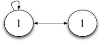
(a) OR-GET network

(b) OR-XOR network

$X$		OR-	OR-
		GET	XOR
00	$\rightarrow$	00	00
01	$\rightarrow$	10	11
10	$\rightarrow$	11	11
11	$\rightarrow$	11	10

Figure 1: *

Transition table for (a), (b)

	c				c
	00	01	10	11	00	01	10	11
$\Pr\!\left(y\right)$	$\nicefrac{{1}}{{4}}$	-	$\nicefrac{{1}}{{4}}$	$\nicefrac{{1}}{{2}}$	$\nicefrac{{1}}{{4}}$	-	$\nicefrac{{1}}{{4}}$	$\nicefrac{{1}}{{2}}$
${\tt ei}(y)$	2.00	-	2.00	1.00	2.00	-	2.00	1.00
$\phi(y)$	1.00	-	2.58	0.58	1.00	-	1.58	1.08

Figure 2: Example OR-GET shows that $\phi(y)$ can exceed not only ${\tt ei}(X~{}\rightarrow~{}y)$, but $\operatornamewithlimits{H}\!\left(X\right)$! A dash means that particular $y$ is unreachable for the network. The concerning $\phi$ values are bolded.

$\phi$ sometimes decreases with duplicate computation. In Figure 4 we take a simple system, AND-ZERO, and duplicate the AND node yielding AND-AND. We see the two systems remain exceedingly similar. Both have $\operatornamewithlimits{H}\!\left(X\right)=2$ and $\operatornamewithlimits{I}\!\left(X\!\mathrel{\mathop{\mathchar 58\relax}}\!Y\right)=0.811$ bits. Likewise, both have two $Y$ states occurring with probability $\nicefrac{{3}}{{4}}$ and $\nicefrac{{1}}{{4}}$ giving ${\tt ei}(X\rightarrow y)$ equal to $0.42$ and $2.00$ bits respectively. However, their $\phi$ values are quite different.

Only knowing that the $\phi$’s for AND-AND and AND-ZERO are different, we’d expect AND-AND to be higher because an AND node “does more” than a ZERO node (simply shutting off). But instead we get the opposite—AND-AND’s highest $\phi$ is less than AND-ZERO’s lowest $\phi$! The ideal measure of integrated information might be invariant or increase under duplicate computation, but it certainly wouldn’t decrease.

(a) AND-ZERO network

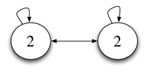
(b) AND-AND network

$X$		AND-	AND-
		ZERO	AND
00	$\rightarrow$	00	00
01	$\rightarrow$	00	00
10	$\rightarrow$	00	00
11	$\rightarrow$	10	11

Figure 3: *

Transition table for (a), (b)

	c				c
	00	01	10	11	00	01	10	11
$\Pr\!\left(y\right)$	$\nicefrac{{3}}{{4}}$	-	$\nicefrac{{1}}{{4}}$	-	$\nicefrac{{3}}{{4}}$	-	-	$\nicefrac{{1}}{{4}}$
${\tt ei}(y)$	0.42	-	2.00	-	0.42	-	-	2.00
$\phi(y)$	0.33	-	1.00	-	0.25	-	-	0.00

Figure 4: Examples AND-ZERO and AND-AND show that $\phi(y)$ sometimes decreases with duplicate computation. Here, the highest $\phi$ of AND-AND is less than the lowest $\phi$ of AND-ZERO. This carries into the average case with AND-ZERO’s $\langle\phi\rangle=0.5$ and AND-AND’s $\langle\phi\rangle=0.189$ bits. A dash means that particular $y$ is unreachable for the network.

$\phi$ does not increase with cooperation among diverse parts. The $\phi$ measure is sometimes described as corresponding to the juxtaposition of “functional segregation” and “functional integration”. In a similar vein, $\phi$ is intuited as corresponding to “interdependence/cooperation among diverse parts”. Figure 5 presents four examples showing that neither intuition is well-captured by the existing $\phi$ measure.

In the first example, SHIFT (Figure 5a), the state of every node is shifted one-step clockwise—nothing more. The nodes are homogeneous and each node is wholly determined by its preceding node. In the three remaining networks (Figures 5b–LABEL:sub@fig:4321), every node is a function of all nodes in the network (including itself). This is to maximize the interdependence/cooperation among the nodes for high “functional integratation”. Having established high cooperation, we increase the diversity or “functional segregation” from Figure 5b to 5d.

By the former intuitions, we’d expect SHIFT (Figure 5a) to have the lowest $\phi$ and 4321 (Figure 5d) to have the highest. But this is not the case. Instead, SHIFT, the network with the least cooperation (every node is a function of one other) and the least diverse mechanisms (all nodes have threshold 1) has a $\phi$ far exceeding the others—SHIFT’s lowest $\phi$ value at two bits dwarfs even the highest $\phi$ values in Figures 5b–LABEL:sub@fig:4321.

SHIFT having the highest integrated information is unexpected, but it’s not outright absurd. SHIFT does have the highest mutual information $\operatornamewithlimits{I}\!\left(X\!\mathrel{\mathop{\mathchar 58\relax}}\!Y\right)$—so the information part is solid. Is SHIFT integrated? Well, in SHIFT each node is wholly determined by an external force (the preceding node); so SHIFT is “integrated” for a sense of the term. Whether it makes sense for SHIFT to have the highest integrated information ultimately comes down to precisely what is meant by the term “integration”. But even accepting that SHIFT is in some sense integrated, example 4321 is integrated for a palpably stronger sense of the term. Therefore, until there’s an argument that the form of integration present in SHIFT is sufficient for awareness, from a purely theoretical perspective it makes sense to prefer 4321 over SHIFT.

(a) SHIFT

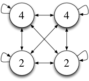
(b) 4422

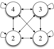
(c) 4322

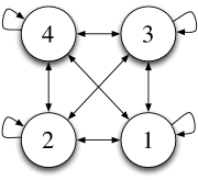
(d) 4321

Network	$\operatornamewithlimits{I}\!\left(X\!\mathrel{\mathop{\mathchar 58\relax}}\!Y\right)$	$\displaystyle\min_{y}\phi(y)$	$\displaystyle\max_{y}\phi(y)$	$\langle\phi\rangle$
SHIFT	4.000	2.000	2.000	2.000
4422	1.198	0.000	0.673	0.424
4322	1.805	0.322	1.586	1.367
4321	2.031	0.322	1.682	1.651

Figure 5: State-dependent $\phi$ and $\langle\phi\rangle$ tell the same story—the $\phi$ value of SHIFT trounces the $\phi$ of the other three networks. A more intuitive complexity measure would instead increase left from to right.

5 A Novel Measure of Irreducibility to a Partition

Our proposed measure $\psi$ quantifies the magnitude of information in $\operatornamewithlimits{I}\!\left(X\!\mathrel{\mathop{\mathchar 58\relax}}\!y\right)$ (eq. (1)) that is irreducible to a partition of the system at time=$0$. We define our measure as,

$$\psi(\mathbf{X}\mathrel{\mathop{\mathchar 58\relax}}y)\equiv\operatornamewithlimits{I}\!\left(X\!\mathrel{\mathop{\mathchar 58\relax}}\!y\right)-\max_{\mathbf{P}}\operatorname{I}_{\cup}\!\left(X^{\mathbf{P}}_{1},\ldots,X^{\mathbf{P}}_{m}\!\mathrel{\mathop{\mathchar 58\relax}}\!y\right)\;,$$ (7)

where $\mathbf{P}$ enumerates over all partitions of set $\mathbf{X}$, and $\operatorname{I}_{\cup}$ is the information about state $y$ conveyed by the “union” across the $m$ parts at time=$0$. To compute the union information $\operatorname{I}_{\cup}$ we use the Partial Information Decomposition (PID) framework. In PID, $\operatorname{I}_{\cup}$ is the inclusion–exclusion dual of $\operatorname{I}_{\cap}$. Thus we can express $\operatorname{I}_{\cup}$ solely in terms of $\operatorname{I}_{\cap}$ by,

$$\operatorname{I}_{\cup}\!\left(X^{\mathbf{P}}_{1},\ldots,X^{\mathbf{P}}_{m}\!\mathrel{\mathop{\mathchar 58\relax}}\!y\right)=\sum_{\mathbf{S}\subseteq\left\{X^{\mathbf{P}}_{1},\ldots,X^{\mathbf{P}}_{m}\right\}}(-1)^{\left|\mathbf{S}\right|+1}\operatorname{I}_{\cap}\!\left(S_{1},\ldots,S_{|\mathbf{S}|}\!\mathrel{\mathop{\mathchar 58\relax}}\!y\right)\;.$$

Conceptually, the intersection information $\operatorname{I}_{\cap}\!\left(S_{1},\ldots,S_{|\mathbf{S}|}\!\mathrel{\mathop{\mathchar 58\relax}}\!y\right)$ quantifies the magnitude of the “same information” about state $y$ conveyed by each $S_{1},\ldots,S_{|\mathbf{S}|}$. Although there’s currently some debate[11, 12] about what is the best $\operatorname{I}_{\cap}$ measure, there’s consensus that the intersection information $n$ arbitrary random variables $Z_{1},\ldots,Z_{n}$ carry about state $y$ must satisfy the following properties:

• Global Positivity: $\operatorname{I}_{\cap}\!\left(Z_{1},\ldots,Z_{n}\!\mathrel{\mathop{\mathchar 58\relax}}\!y\right)\geq 0$.

• Weak Symmetry: $\operatorname{I}_{\cap}\!\left(Z_{1},\ldots,Z_{n}\!\mathrel{\mathop{\mathchar 58\relax}}\!y\right)$ is invariant under reordering $Z_{1},\ldots,Z_{n}$.

• Self-Redundancy: $\operatorname{I}_{\cap}\!\left(Z_{1}\!\mathrel{\mathop{\mathchar 58\relax}}\!y\right)=\operatornamewithlimits{I}\!\left(Z_{1}\!\mathrel{\mathop{\mathchar 58\relax}}\!y\right)=\operatorname{D_{KL}}\!\left[\Pr\!\left(Z_{1}|y\right)\middle\|\,\Pr\!\left(Z_{1}\right)\right]$. The intersection information a single predictor $Z_{1}$ conveys about the target state $y$ is equal to the “specific surprise”[9].

• Strong Monotonicity: $\operatorname{I}_{\cap}\!\left(Z_{1},\ldots,Z_{n},W\!\mathrel{\mathop{\mathchar 58\relax}}\!y\right)\leq\operatorname{I}_{\cap}\!\left(Z_{1},\ldots,Z_{n}\!\mathrel{\mathop{\mathchar 58\relax}}\!y\right)$ with equality if there exists $Z_{i}\in\{Z_{1},\ldots,Z_{n}\}$ such that $\operatornamewithlimits{I}\!\left(WZ_{i}\!\mathrel{\mathop{\mathchar 58\relax}}\!y\right)=\operatornamewithlimits{I}\!\left(W\!\mathrel{\mathop{\mathchar 58\relax}}\!y\right)$ where $WZ_{i}$ is the joint random variable (cartesian product) of $W$ and $Z_{i}$.

• Equivalence-Class Invariance: $\operatorname{I}_{\cap}\!\left(Z_{1},\ldots,Z_{n}\!\mathrel{\mathop{\mathchar 58\relax}}\!y\right)$ is invariant under substituting $Z_{i}$ (for any $i=1,\ldots,n$) by an informationally equivalent random variable[12]. Similarly, $\operatorname{I}_{\cap}\!\left(Z_{1},\ldots,Z_{n}\!\mathrel{\mathop{\mathchar 58\relax}}\!y\right)$ is invariant under substituting state $y$ for state $w$ if $\Pr\!\left(w|y\right)=\Pr\!\left(y|w\right)=1$.

Now we take a less common course—instead of choosing a particular $\operatorname{I}_{\cap}$ that satisfies the above properties, we will simply use the properties above directly to bound the range of possible $\psi$ values. Leveraging $\mathbf{\left(M_{1}\right)}$, $\mathbf{\left(S_{0}\right)}$, and $\mathbf{(SR)}$, eq. (7) simplifies to,

$$\begin{split}\psi(\mathbf{X}\mathrel{\mathop{\mathchar 58\relax}}y)&=\operatornamewithlimits{I}\!\left(X\!\mathrel{\mathop{\mathchar 58\relax}}\!y\right)-\max_{A\subset\mathbf{X}}\operatorname{I}_{\cup}\!\left(A,B\!\mathrel{\mathop{\mathchar 58\relax}}\!y\right)\\ &=\operatornamewithlimits{I}\!\left(X\!\mathrel{\mathop{\mathchar 58\relax}}\!y\right)-\max_{A\subset\mathbf{X}}\left[\operatornamewithlimits{I}\!\left(A\!\mathrel{\mathop{\mathchar 58\relax}}\!y\right)+\operatornamewithlimits{I}\!\left(B\!\mathrel{\mathop{\mathchar 58\relax}}\!y\right)-\operatorname{I}_{\cap}\!\left(A,B\!\mathrel{\mathop{\mathchar 58\relax}}\!y\right)\right]\;,\end{split}$$ (8)

where $A\not=\emptyset$ and $B\equiv\mathbf{X}\setminus A$.

From eq. (8), the only undefined term is $\operatorname{I}_{\cap}\!\left(A,B\!\mathrel{\mathop{\mathchar 58\relax}}\!y\right)$. Leveraging $\mathbf{(GP)}$, $\mathbf{\left(M_{1}\right)}$, and $\mathbf{(SR)}$, we can bound it by,

$$0\leq\operatorname{I}_{\cap}\!\left(A,B\!\mathrel{\mathop{\mathchar 58\relax}}\!y\right)\leq\min\left[\operatornamewithlimits{I}\!\left(A\!\mathrel{\mathop{\mathchar 58\relax}}\!y\right),\operatornamewithlimits{I}\!\left(B\!\mathrel{\mathop{\mathchar 58\relax}}\!y\right)\right]\;.$$ (9)

Finally, we bound $\psi$ by plugging in the above bounds on $\operatorname{I}_{\cap}\!\left(A,B\!\mathrel{\mathop{\mathchar 58\relax}}\!y\right)$ into eq. (8). With some algebra and leveraging assumption (B), this yields the following bounds for $\psi$,

$$\begin{split}\psi_{\min}\!\left(\mathbf{X}\mathrel{\mathop{\mathchar 58\relax}}y\right)&=\min_{A\subset\mathbf{X}}\operatorname{D_{KL}}\!\left[\Pr\!\left(X\middle|y\right)\middle\|\,\Pr\!\left(A|y\right)\Pr\!\left(B|y\right)\right]\\ \psi_{\max}\!\left(\mathbf{X}\mathrel{\mathop{\mathchar 58\relax}}y\right)&=\min_{i\in\{1,\ldots,n\}}\operatorname{D_{KL}}\!\left[\Pr\!\left(X\middle|y\right)\middle\|\,\Pr\!\left(X_{i}\right)\Pr\!\left(X_{\sim i}\middle|y\right)\right]\;,\end{split}$$ (10)

where $X_{\sim i}$ is the random variable of all nodes in $X$ excluding node $i$. Then,
$\psi_{\min}(\mathbf{X}\mathrel{\mathop{\mathchar 58\relax}}y)\leq\psi(\mathbf{X}\mathrel{\mathop{\mathchar 58\relax}}y)\leq\psi_{\max}(\mathbf{X}\mathrel{\mathop{\mathchar 58\relax}}y)$.

5.1 Stateless $\psi$ is $\langle\psi\rangle$

We define $\langle\psi\rangle$ analogous to $\phi$ per Section 3.1. To compute $\langle\psi\rangle$ we weaken the properties in Section 5 so that they only apply to the average case, i.e., the properties $\mathbf{(GP)}$, $\mathbf{\left(M_{1}\right)}$, $\mathbf{\left(S_{0}\right)}$, $\mathbf{(SR)}$, and $\mathbf{(Eq)}$ don’t have to apply for each $\operatorname{I}_{\cap}\!\left(Z_{1},\ldots,Z_{n}\!\mathrel{\mathop{\mathchar 58\relax}}\!y\right)$, but merely for the average case $\operatorname{I}_{\cap}\!\left(Z_{1},\ldots,Z_{n}\!\mathrel{\mathop{\mathchar 58\relax}}\!Y\right)$.

Via the same algebra from eq. (8), $\langle\psi\rangle$ simplifies to,

$$\begin{split}\langle\psi\rangle(X_{1},\ldots,X_{n}\mathrel{\mathop{\mathchar 58\relax}}Y)&\equiv\operatornamewithlimits{I}\!\left(X\!\mathrel{\mathop{\mathchar 58\relax}}\!Y\right)-\max_{\mathbf{P}}\operatorname{I}_{\cup}\!\left(X^{\mathbf{P}}_{1},\ldots,X^{\mathbf{P}}_{m}\!\mathrel{\mathop{\mathchar 58\relax}}\!Y\right)\\ &=\operatornamewithlimits{I}\!\left(X\!\mathrel{\mathop{\mathchar 58\relax}}\!Y\right)-\max_{A\subset\mathbf{X}}\operatorname{I}_{\cup}\!\left(A,B\!\mathrel{\mathop{\mathchar 58\relax}}\!Y\right)\\ &=\operatornamewithlimits{I}\!\left(X\!\mathrel{\mathop{\mathchar 58\relax}}\!Y\right)-\max_{A\subset\mathbf{X}}\left[\operatornamewithlimits{I}\!\left(A\!\mathrel{\mathop{\mathchar 58\relax}}\!Y\right)+\operatornamewithlimits{I}\!\left(B\!\mathrel{\mathop{\mathchar 58\relax}}\!Y\right)-\operatorname{I}_{\cap}\!\left(A,B\!\mathrel{\mathop{\mathchar 58\relax}}\!Y\right)\right]\;,\end{split}$$ (11)

where $A\not=\emptyset$ and $B\equiv\mathbf{X}\setminus A$. Using the weakened properties, we likewise have $0\leq\operatorname{I}_{\cap}\!\left(A,B\!\mathrel{\mathop{\mathchar 58\relax}}\!Y\right)\leq\min\left[\operatornamewithlimits{I}\!\left(A\!\mathrel{\mathop{\mathchar 58\relax}}\!Y\right),\operatornamewithlimits{I}\!\left(B\!\mathrel{\mathop{\mathchar 58\relax}}\!Y\right)\right]$. Plugging in these $\operatorname{I}_{\cap}$ bounds yields the following bounds $\langle\psi\rangle$,

$$\begin{split}\langle\psi\rangle_{\min}\!\left(\mathbf{X}\mathrel{\mathop{\mathchar 58\relax}}Y\right)&=\min_{A\subset\mathbf{X}}\operatornamewithlimits{I}\!\left(A\!\mathrel{\mathop{\mathchar 58\relax}}\!B\middle|Y\right)\\ \langle\psi\rangle_{\max}\!\left(\mathbf{X}\mathrel{\mathop{\mathchar 58\relax}}Y\right)&=\min_{i\in\{1,\ldots,n\}}\operatorname{D_{KL}}\!\left[\Pr\!\left(X,Y\right)\middle\|\,\Pr\!\left(X_{\sim i},Y\right)\Pr\!\left(X_{i}\right)\right]\;,\end{split}$$ (12)

where $X_{\sim i}$ is the random variable of all nodes in $X$ excluding node $i$. Then,
$\langle\psi\rangle_{\min}(\mathbf{X}\mathrel{\mathop{\mathchar 58\relax}}Y)\leq\langle\psi\rangle(\mathbf{X}\mathrel{\mathop{\mathchar 58\relax}}Y)\leq\langle\psi\rangle_{\max}(\mathbf{X}\mathrel{\mathop{\mathchar 58\relax}}Y)$.

6 Contrasting $\psi$ versus $\phi$

Theoretical benefits of $\psi$. The overarching theoretical benefit is that $\psi$ is entrenched within the rigorous Partial Information Decomposition framework[13]. PID builds a principled irreducibility measure from a redundancy measure $\operatorname{I}_{\cap}$. Here we only take the most accepted properties of $\operatorname{I}_{\cap}$ to bound $\psi$ from above and below. As the complexity community converges on the additional properties $\operatorname{I}_{\cap}$ must satisfy[11, 12], the derived bounds on $\psi$ will tighten.

There are four benefits of $\psi$’s principled underpinning. First, whereas $\phi(y)$ can exceed the entropy of the whole system, i.e., $\phi(y)\not\leq\operatornamewithlimits{H}\!\left(X\right)$, $\psi(y)$ is bounded by specific-surprise, i.e., $\psi(y)~{}\leq~{}\operatornamewithlimits{I}\!\left(X\!\mathrel{\mathop{\mathchar 58\relax}}\!y\right)=\operatorname{D_{KL}}\!\left[\Pr\!\left(X|y\right)\middle\|\,\Pr\!\left(X\right)\right]$. This gives $\psi$ the natural info-theoretic interpretation for the state-dependent case which $\phi$ lacks. Second, PID provides justification for $\psi$ not needing a MIP normalization and thus eliminates a longstanding ambiguity about $\phi$[14]. Third, PID is a flexible framework that enables quantifying irreducibility to overlapping parts should we decide to explore it.

One final perk is that $\psi$ is already substantially faster to compute. Whereas computing $\phi$ scales $O(n!)$, computing $\psi$ scales $O(2^{n})$—a substantial improvement that may improve even further as the complexity community converges on additional properties of $\operatorname{I}_{\cap}$.

Behavioral differences between $\psi$ and $\phi$. The first row in Figure 6 shows two ways a network can be irreducible to atomic elements (the nodes) yet still reducible to disjoint parts. Compare AND-ZERO (Figure 6g) to AND-ZERO+KEEP (Figure 6a). Although AND-ZERO is irreducible, AND-ZERO+KEEP reduces to the bipartition separating the AND-ZERO component and the KEEP node. This reveals how fragile measures like $\psi$ and $\phi$ are—add a single disconnected node and they plummet to zero. Example 2x AND-ZERO (Figure 6b) shows that a wholly reducible network can be composed entirely of irreducible parts.

Example KEEP-KEEP (Figure 6c) highlights the only known relative drawback of $\psi$—$\psi$’s current upperbound is painfully loose. The desired irreducibility for KEEP-KEEP is zero bits, and indeed, $\psi_{\min}$ is $0$ bits—but $\psi_{\max}$ is a monstrous $1$ bit! We rightly expect tighter bounds for such easy examples like KEEP-KEEP. Tighter bounds on $\operatorname{I}_{\cap}$ (and thus $\psi$) is an area of active research but as-is the bounds are loose.

Example GET-GET (Figure 6d) epitomizes the most striking difference between $\psi$ and $\phi$. By property $\mathbf{(Eq)}$, the $\psi$ values for KEEP-KEEP and GET-GET are provably equal (making the desired $\psi$ for GET-GET zero bits), yet their $\phi$ values couldn’t be more different. Although the $\phi$ for KEEP-KEEP is zero, the $\phi$ for GET-GET is the maximal (!) two bits of irreducibility. Whereas $\psi$ views GET nodes as non-integrative, $\phi$ views GET nodes as maximally integrative.

This begs the question—should GETs be integrative? It’s sensible for GETs to be mildly integrative, but the logic of partitioning the system forces us to choose between GETs being non-integrative (akin to a KEEP) or maximally integrative. To resolve this dilemma this we return to Figure 5. The primary benefit of $\psi$ making KEEPs and GETs equivalent is that $\psi$ is zero for chains of GETs such as the SHIFT network (Figure 5a). This enables $\psi$ to better match our intuition for “cooperation among diverse parts”. For example, in Figure 5 the network with the highest $\phi$ is the counter-intuitive SHIFT, but the network with the highest $\psi$ is the more sensible 4321 (see table in Figure 6). With these examples in mind, we personally believe GETs being non-integrative is the better choice.

The third row in Figure 6 shows how $\psi$ and $\phi$ respectively treat self-connections. In ANDtriplet (Figure 6e) and iso-ANDtriplet (Figure 6f) each node integrates information about two nodes. The only difference is that in ANDtriplet each node integrates information about two other nodes, while in iso-ANDtriplet each node integrates information is about itself and one other.

Just as $\psi$ views KEEP and GET nodes equivalently, $\psi$ views self and cross connections equivalently. In fact, by property $\mathbf{(Eq)}$ the $\psi$ values for ANDtriplet and iso-ANDtriplet are provably equal. Alternatively, $\phi$ considers self and cross connections differently in that $\phi$ can only decrease when adding a self-connection. As such, the $\phi$ for iso-ANDtriplet is less than ANDtriplet.

The fourth row in Figure 6 shows this same self-connections business carrying over to duplicate computations. Although AND-AND (Figure 6h) and AND-ZERO (Figure 6g) perform the same computation, AND-AND has an additional self-connection that pushes AND-AND’s $\phi$ below that of AND-ZERO. By $\mathbf{(Eq)}$, the $\psi$ values of AND-ZERO and AND-AND are provably equal.

7 Conclusion

Regardless of any connection to consciousness, purely as a measure of functional irreducibility we have three concerns about $\phi$: (1) state-dependent $\phi$ can exceed the entropy of the entire system; (2) $\phi$ often decreases with duplicate computation; (3) $\phi$ doesn’t match the intuition of “cooperation among diverse parts”.

We introduced a new irreducibility measure, $\psi$, that solves all three concerns but otherwise stays close to the original spirit of $\phi$—i.e., the quantification of a system’s irreducibility to disjoint parts. Based in Partial Information Decomposition, $\psi$ has other desirable properties such as not needing a MIP normalization and being substantially faster to compute. We then contrasted $\psi$ versus $\phi$ in binary networks.

Although we endorse $\psi$ over $\phi$, the $\psi$ measure remains imperfect. The most notable areas for improvement are:

1. The current $\psi$ bounds are too loose. We need to tighten the $\operatorname{I}_{\cap}$ bounds (eq. (9)), which will tighten the derived bounds on $\psi$ and $\langle\psi\rangle$.

2. Justify why a measure of conscious experience should prefer irreducibility to disjoint parts over irreducibility to overlapping parts.

3. Reformalize the work on qualia in [2] using $\psi$ or comparable measure.

4. Although not specific to $\psi$, there needs to be a stronger justification for the chosen distribution on $X$ (see Appendix E).

Our introduced $\psi$ measure effortlessly generalizes to the quantum case simply by replacing all instances of Shannon mutual information in eq. (8) with von Neumann (quantum) information. This “quantum $\psi$” is a quantum infotheoretic measure that remains much more faithful to its parents [1, 3] than Tegmark’s innovative perceptronium implementation[15].

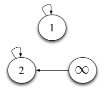
(a) AND-ZERO+KEEP

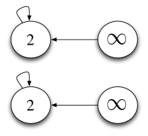
(b) 2x AND-ZERO

(c) KEEP-KEEP

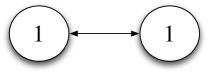
(d) GET-GET

(e) ANDtriplet

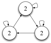
(f) iso-ANDtriplet

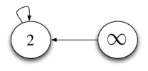
(g) AND-ZERO

(h) AND-AND

Network	$\operatornamewithlimits{I}\!\left(X\!\mathrel{\mathop{\mathchar 58\relax}}\!Y\right)$	$\langle\phi\rangle$	$\langle\psi\rangle_{\min}$	$\langle\psi\rangle_{\max}$
AND-ZERO+KEEP LABEL:sub@fig:AZK	1.81	0	0	0.50
2x AND-ZERO LABEL:sub@fig:AZ_AZ	1.62	0	0	0.50
KEEP-KEEP LABEL:sub@fig:KK_one	2.00	0	0	1.00
GET-GET LABEL:sub@fig:GG_one	2.00	2.00	0	1.00
ANDtriplet LABEL:sub@fig:AAA_one	2.00	2.00	0.16	0.75
iso-ANDtriplet LABEL:sub@fig:rArArA_one	2.00	1.07	0.16	0.75
AND-ZERO LABEL:sub@fig:AZ_one	0.81	0.50	0.19	0.50
AND-AND LABEL:sub@fig:AA_one	0.81	0.19	0.19	0.50
SHIFT (Fig. 5a)	4.00	2.00	0	1.00
4422 (Fig. 5b)	1.20	0.42	0.33	0.50
4322 (Fig. 5c)	1.81	1.37	0.68	0.88
4321 (Fig. 5d)	2.03	1.65	0.78	1.00

Figure 6: Contrasting $\langle\phi\rangle$ versus $\langle\psi\rangle$ for exemplary networks.

Appendix

Appendix A Reading the Network Diagrams

We present eight doublet networks and their transition tables so you can see how the network diagram specifies the transition table. Figure 7 shows eight network diagrams to build your intuition. The number inside each node is that node’s activation threshold. A node updates to 1 (conceptually an “ON”) if there at least as many of inputs ON as its activation threshold; e.g. a node with an inscribed 2 updates to a 1 if two or more incoming wires are ON. An activation threshold of $\infty$ means the node always updates to 0 (conceptually an “OFF”). A binary string denotes the state of the network, read left to right.

We take the AND-ZERO network (Figure 7g) as an example. Although the AND-ZERO network can never output 01 or 11 (Figure 1b), we still consider states 01, 11 as equally possible states at time=0. This is because $X$ is uniformly distributed per assumption (B).

(a) ZERO-ZERO

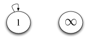
(b) KEEP-ZERO

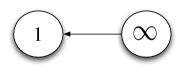
(c) GET-ZERO

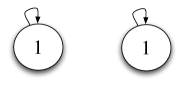
(d) KEEP-KEEP

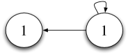
(e) GET-KEEP

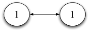
(f) GET-GET

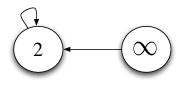
(g) AND-ZERO

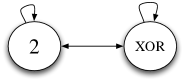
(h) AND-XOR

$X$		ZERO-	KEEP-	GET-	KEEP-	GET-	GET-	AND-	AND-
		ZERO	ZERO	ZERO	KEEP	KEEP	GET	ZERO	XOR
00	$\rightarrow$	00	00	00	00	00	00	00	00
01	$\rightarrow$	00	00	10	01	11	10	00	01
10	$\rightarrow$	00	10	00	10	00	01	00	01
11	$\rightarrow$	00	10	10	11	11	11	10	10

Figure 7: Eight doublet networks with transition tables.

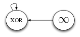
(a) XOR-ZERO

(b) XOR-KEEP

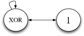
(c) XOR-GET

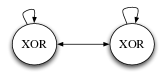
(d) XOR-XOR

(e) XOR-AND

$X$		XOR-	XOR-	XOR-	XOR-	XOR-
		ZERO	KEEP	GET	XOR	AND
00	$\rightarrow$	00	00	00	00	00
01	$\rightarrow$	10	11	10	11	10
10	$\rightarrow$	10	10	11	11	10
11	$\rightarrow$	00	01	01	00	01

Network	$\operatornamewithlimits{I}\!\left(X\!\mathrel{\mathop{\mathchar 58\relax}}\!Y\right)$	$\langle\phi\rangle$	$\langle\psi\rangle_{\min}$	$\langle\psi\rangle_{\max}$
ZERO-ZERO (Fig. 7a)	0	0	0	0
KEEP-ZERO (Fig. 7b)	1.0	0	0	0
KEEP-KEEP (Fig. 7d)	2.0	0	0	1.0
GET-ZERO (Fig. 7c)	1.0	1.0	0	0
GET-KEEP (Fig. 7e)	1.0	0	0	0
GET-GET (Fig. 7f)	2.0	2.0	0	1.0
AND-ZERO (Fig. 3a)	0.811	0.5	0.189	0.5
AND-KEEP	1.5	0.189	0	0.5
AND-GET	1.5	1.189	0	0.5
AND-AND (Fig. 3b)	0.811	0.189	0.189	0.5
AND-XOR (Fig. 7h)	1.5	1.189	0.5	1.0
XOR-ZERO LABEL:sub@fig:XZ	1.0	1.0	1.0	1.0
XOR-KEEP LABEL:sub@fig:XK	2.0	1.0	0	1.0
XOR-GET LABEL:sub@fig:XG	2.0	2.0	0	1.0
XOR-AND LABEL:sub@fig:XA	1.5	1.189	0.5	1.0
XOR-XOR LABEL:sub@fig:XX	1.0	1.0	1.0	1.0

Figure 8: Networks, transition tables, and measures for the diagnostic doublets.

Appendix B Necessary Proofs

B.1 Proof that Max Union of Bipartitions Covers All Partitions

Lemma 1.

Given properties $\mathbf{\left(S_{0}\right)}$ and $\mathbf{\left(M_{1}\right)}$, the maximum union information conveyed by a partition of predictors $\mathbf{X}=\{X_{1},\ldots,X_{n}\}$ about state $y$ equals the maximum union information conveyed by a bipartition of $\mathbf{X}$ about state $y$.

Proof.

We prove that the maximum information conveyed by a Partition, $\textnormal{IcP}(\mathbf{X}\mathrel{\mathop{\mathchar 58\relax}}y)$, equals the maximum information conveyed by a Bipartition, $\textnormal{IcB}(\mathbf{X}\mathrel{\mathop{\mathchar 58\relax}}y)$ by showing,

$$\textnormal{IcP}(\mathbf{X}\mathrel{\mathop{\mathchar 58\relax}}y)\leq\textnormal{IcB}(\mathbf{X}\mathrel{\mathop{\mathchar 58\relax}}y)\leq\textnormal{IcP}(\mathbf{X}\mathrel{\mathop{\mathchar 58\relax}}y)\;.$$ (13)

First we show that $\textnormal{IcB}(\mathbf{X}\mathrel{\mathop{\mathchar 58\relax}}y)\leq\textnormal{IcP}(\mathbf{X}\mathrel{\mathop{\mathchar 58\relax}}y)$. By their definitions.

$$\textnormal{IcP}(\mathbf{X}\mathrel{\mathop{\mathchar 58\relax}}y) \equiv\max_{\mathbf{P}}\operatorname{I}_{\cup}\!\left(\mathbf{P}\!\mathrel{\mathop{\mathchar 58\relax}}\!y\right)$$

$$\textnormal{IcB}(\mathbf{X}\mathrel{\mathop{\mathchar 58\relax}}y) \equiv\max_{\begin{subarray}{c}\mathbf{P}\\ |\mathbf{P}|=2\end{subarray}}\operatorname{I}_{\cup}\!\left(\mathbf{P}\!\mathrel{\mathop{\mathchar 58\relax}}\!y\right)\;,$$

where $\mathbf{P}$ enumerates over all partitions of set $\mathbf{X}$.

By removing the restriction that $|\mathbf{P}|=2$ from the maximization in IcB we arrive at IcP. As removing a restriction can only increase the maximum, thus $\textnormal{IcB}(\mathbf{X}\mathrel{\mathop{\mathchar 58\relax}}y)~{}\leq~{}\textnormal{IcP}(\mathbf{X}\mathrel{\mathop{\mathchar 58\relax}}y)$.

Next we show that $\textnormal{IcP}(\mathbf{X}\mathrel{\mathop{\mathchar 58\relax}}y)\leq\textnormal{IcB}\left(\mathbf{X}\mathrel{\mathop{\mathchar 58\relax}}y\right)$. Meaning we must show that,

$$\max_{\mathbf{P}}\;\operatorname{I}_{\cup}\!\left(\mathbf{P}\!\mathrel{\mathop{\mathchar 58\relax}}\!y\right)\leq\max_{\begin{subarray}{c}\mathbf{P}\\ |\mathbf{P}|=2\end{subarray}}\operatorname{I}_{\cup}\!\left(\mathbf{P}\!\mathrel{\mathop{\mathchar 58\relax}}\!y\right)\;.$$ (14)

Without loss of generality, we choose an arbitrary subset/part $S\subset\mathbf{X}$. This yields the bipartition of parts $\{S,\mathbf{X}\setminus S\}$. We then further partition the second part, $\mathbf{X}\setminus S$, into $k$ (disjoint) subparts denoted $T_{1},\ldots,T_{k}$ where $2\leq k\leq n-\left|S\right|$ creating an arbitrary partition $\mathbf{P}=\{S,T_{1},\ldots,T_{k}\}$. We now need to show that,

$$\operatorname{I}_{\cup}\!\left(S,T_{1},\ldots,T_{k}\!\mathrel{\mathop{\mathchar 58\relax}}\!y\right)\leq\operatorname{I}_{\cup}\!\left(S,\mathbf{X}\setminus S\!\mathrel{\mathop{\mathchar 58\relax}}\!y\right)\;.$$

By $\mathbf{\left(M_{1}\right)}$ equality condition, we can append each subcomponent $T_{1},\ldots,T_{k}$ to $\{S,\mathbf{X}\setminus S\}$ without changing the union-information because for each $T_{i}$, $\operatornamewithlimits{H}\!\left(T_{i}|\mathbf{X}\setminus S\right)=0$. Then applying $\mathbf{\left(S_{0}\right)}$ we re-order the parts so that $S,T_{1},\ldots,T_{k}$ come first. This yields,

$$\operatorname{I}_{\cup}\!\left(S,T_{1},\ldots,T_{k}\!\mathrel{\mathop{\mathchar 58\relax}}\!y\right)\leq\operatorname{I}_{\cup}\!\left(S,T_{1},\ldots,T_{k},\mathbf{X}\setminus S\!\mathrel{\mathop{\mathchar 58\relax}}\!y\right)\;.$$

Applying $\mathbf{\left(M_{1}\right)}$ inequality condition, adding the predictor $\mathbf{X}\setminus S$ can only increase the union information. Therefore we prove eq. (14), which proves eq. (13), that $\textnormal{IcP}(\mathbf{X}~{}\mathrel{\mathop{\mathchar 58\relax}}~{}y)~{}=~{}\textnormal{IcB}(\mathbf{X}~{}\mathrel{\mathop{\mathchar 58\relax}}~{}y)$. ∎

B.2 Bounds on $\psi(X_{1},\ldots,X_{n}\mathrel{\mathop{\mathchar 58\relax}}y)$

Lemma 2.

Given $\mathbf{\left(M_{1}\right)}$, $\mathbf{(SR)}$ and the predictors $X_{1},\ldots,X_{n}$ are independent, i.e., $\operatornamewithlimits{H}\!\left(X\right)=\sum_{i=1}^{n}\operatornamewithlimits{H}\!\left(X_{i}\right)$, then,

$$\psi(X_{1},\ldots,X_{n}\mathrel{\mathop{\mathchar 58\relax}}y)\leq\min_{i\in\{1,\ldots,n\}}\operatorname{D_{KL}}\!\left[\Pr\!\left(X\middle|y\right)\middle\|\,\Pr\!\left(X_{i}\right)\Pr\!\left(X_{\sim i}\middle|y\right)\right]\;.$$

Proof.

Applying $\mathbf{\left(M_{1}\right)}$ inequality condition, we have $\operatorname{I}_{\cap}\!\left(A,B\!\mathrel{\mathop{\mathchar 58\relax}}\!y\right)\leq\min\left[\operatornamewithlimits{I}\!\left(A\!\mathrel{\mathop{\mathchar 58\relax}}\!y\right),\operatornamewithlimits{I}\!\left(B\!\mathrel{\mathop{\mathchar 58\relax}}\!y\right)\right]$. Via the inclusion-exclusion rule, this entails $\operatorname{I}_{\cup}\!\left(A,B\!\mathrel{\mathop{\mathchar 58\relax}}\!y\right)\geq\max\left[\operatornamewithlimits{I}\!\left(A\!\mathrel{\mathop{\mathchar 58\relax}}\!y\right),\operatornamewithlimits{I}\!\left(B\!\mathrel{\mathop{\mathchar 58\relax}}\!y\right)\right]$, and we use this to upperbound $\psi(X_{1},\ldots,X_{n}\mathrel{\mathop{\mathchar 58\relax}}y)$. The random variable $A\not=\emptyset$, $B\equiv\mathbf{X}\setminus A$, and $AB\equiv X$.

$$\psi(X_{1},\ldots,X_{n}\mathrel{\mathop{\mathchar 58\relax}}y) =\operatornamewithlimits{I}\!\left(X\!\mathrel{\mathop{\mathchar 58\relax}}\!y\right)-\max_{A\subset\mathbf{X}}\operatorname{I}_{\cup}\!\left(A,B\!\mathrel{\mathop{\mathchar 58\relax}}\!y\right)$$

$$\leq\operatornamewithlimits{I}\!\left(X\!\mathrel{\mathop{\mathchar 58\relax}}\!y\right)-\max_{A\subset\mathbf{X}}\max\left[\operatornamewithlimits{I}\!\left(A\!\mathrel{\mathop{\mathchar 58\relax}}\!y\right),\operatornamewithlimits{I}\!\left(B\!\mathrel{\mathop{\mathchar 58\relax}}\!y\right)\right]$$

By symmetry of complementary bipartitions, every $$B A$$ will be an at some

point. So we can drop the $$B$$ term.

$$=\operatornamewithlimits{I}\!\left(X\!\mathrel{\mathop{\mathchar 58\relax}}\!y\right)-\max_{A\subset\mathbf{X}}\operatornamewithlimits{I}\!\left(A\!\mathrel{\mathop{\mathchar 58\relax}}\!y\right)\;.$$

For two parts $A$ and $A^{\prime}$ such that $\operatornamewithlimits{H}\!\left(A|A^{\prime}\right)=0$, $\operatornamewithlimits{I}\!\left(A\!\mathrel{\mathop{\mathchar 58\relax}}\!y\right)\leq\operatornamewithlimits{I}\!\left(A^{\prime}\!\mathrel{\mathop{\mathchar 58\relax}}\!y\right)$. Therefore there will always be a maximizing subset of $\mathbf{X}$ of size $n-1$.

$$\psi(X_{1},\ldots,X_{n}\mathrel{\mathop{\mathchar 58\relax}}y) \leq\operatornamewithlimits{I}\!\left(X\!\mathrel{\mathop{\mathchar 58\relax}}\!y\right)-\max_{\begin{subarray}{c}A\subset\mathbf{X}\\ |A|=n-1\end{subarray}}\operatornamewithlimits{I}\!\left(A\!\mathrel{\mathop{\mathchar 58\relax}}\!y\right)$$

$$=\operatornamewithlimits{I}\!\left(X\!\mathrel{\mathop{\mathchar 58\relax}}\!y\right)-\max_{i\in\{1,\ldots,n\}}\operatornamewithlimits{I}\!\left(X_{\sim i}\!\mathrel{\mathop{\mathchar 58\relax}}\!y\right)$$

$$=\min_{i\in\{1,\ldots,n\}}\operatornamewithlimits{I}\!\left(X\!\mathrel{\mathop{\mathchar 58\relax}}\!y\right)-\operatornamewithlimits{I}\!\left(X_{\sim i}\!\mathrel{\mathop{\mathchar 58\relax}}\!y\right)$$

$$=\min_{i\in\{1,\ldots,n\}}\operatornamewithlimits{I}\!\left(X_{i}\!\mathrel{\mathop{\mathchar 58\relax}}\!y\middle|X_{\sim i}\right)$$

$$=\min_{i\in\{1,\ldots,n\}}\operatorname{D_{KL}}\!\left[\Pr\!\left(X\middle|y\right)\middle\|\,\Pr\!\left(X_{i}\middle|X_{\sim i}\right)\Pr\!\left(X_{\sim i}\middle|y\right)\right]\;.$$

Now applying that the predictors $\mathbf{X}$ are independent, $\Pr\!\left(x_{i}\middle|x_{\sim i}\right)=\Pr\!\left(x_{i}\right)$. This leaves,

$$\psi(X_{1},\ldots,X_{n}\mathrel{\mathop{\mathchar 58\relax}}y)\leq\min_{i\in\{1,\ldots,n\}}\operatorname{D_{KL}}\!\left[\Pr\!\left(X\middle|y\right)\middle\|\,\Pr\!\left(X_{i}\right)\Pr\!\left(X_{\sim i}\middle|y\right)\right]\;.$$

∎

Lemma 3.

Given $\mathbf{(GP)}$, $\mathbf{(SR)}$ and predictors $X_{1},\ldots,X_{n}$ are independent, i.e., $\operatornamewithlimits{H}\!\left(X\right)=\sum_{i=1}^{n}\operatornamewithlimits{H}\!\left(X_{i}\right)$, then,

$$\begin{split}\psi(X_{1},\ldots,X_{n}\mathrel{\mathop{\mathchar 58\relax}}y)&\geq\min_{A\subset\mathbf{X}}\operatornamewithlimits{I}\!\left(A\!\mathrel{\mathop{\mathchar 58\relax}}\!B\middle|y\right)\\ &=\min_{A\subset\mathbf{X}}\operatorname{D_{KL}}\!\left[\Pr\!\left(X|y\right)\middle\|\,\Pr\!\left(A|y\right)\Pr\!\left(B|y\right)\right]\;.\end{split}$$

Proof.

First, from the definition of $\operatorname{I}_{\cup}$, $\operatorname{I}_{\cup}\!\left(A,B\!\mathrel{\mathop{\mathchar 58\relax}}\!y\right)=\operatornamewithlimits{I}\!\left(A\!\mathrel{\mathop{\mathchar 58\relax}}\!y\right)+\operatornamewithlimits{I}\!\left(B\!\mathrel{\mathop{\mathchar 58\relax}}\!y\right)-\operatorname{I}_{\cap}\!\left(A,B\!\mathrel{\mathop{\mathchar 58\relax}}\!y\right)$. Then applying $\mathbf{(GP)}$, we have $\operatorname{I}_{\cup}\!\left(A,B\!\mathrel{\mathop{\mathchar 58\relax}}\!y\right)\leq\operatornamewithlimits{I}\!\left(A\!\mathrel{\mathop{\mathchar 58\relax}}\!y\right)+\operatornamewithlimits{I}\!\left(B\!\mathrel{\mathop{\mathchar 58\relax}}\!y\right)$. We use this to lowerbound $\psi(X_{1},\ldots,X_{n}\mathrel{\mathop{\mathchar 58\relax}}y)$. The random variable $A\not=\emptyset$, $B\equiv\mathbf{X}\setminus A$, and $AB\equiv X$.

$$\psi(X_{1},\ldots,X_{n}\mathrel{\mathop{\mathchar 58\relax}}y) =\operatornamewithlimits{I}\!\left(X\!\mathrel{\mathop{\mathchar 58\relax}}\!y\right)-\max_{A\subset\mathbf{X}}\operatorname{I}_{\cup}\!\left(A,B\!\mathrel{\mathop{\mathchar 58\relax}}\!y\right)$$

$$\geq\operatornamewithlimits{I}\!\left(X\!\mathrel{\mathop{\mathchar 58\relax}}\!y\right)-\max_{A\subset\mathbf{X}}\left[\operatornamewithlimits{I}\!\left(A\!\mathrel{\mathop{\mathchar 58\relax}}\!y\right)+\operatornamewithlimits{I}\!\left(B\!\mathrel{\mathop{\mathchar 58\relax}}\!y\right)\right]$$

$$=\min_{A\subset\mathbf{X}}\operatornamewithlimits{I}\!\left(AB\!\mathrel{\mathop{\mathchar 58\relax}}\!y\right)-\operatornamewithlimits{I}\!\left(A\!\mathrel{\mathop{\mathchar 58\relax}}\!y\right)-\operatornamewithlimits{I}\!\left(B\!\mathrel{\mathop{\mathchar 58\relax}}\!y\right)$$

$$=\min_{A\subset\mathbf{X}}\operatornamewithlimits{I}\!\left(A\!\mathrel{\mathop{\mathchar 58\relax}}\!y|B\right)-\operatornamewithlimits{I}\!\left(A\!\mathrel{\mathop{\mathchar 58\relax}}\!y\right)$$

$$=\min_{A\subset\mathbf{X}}\operatorname{D_{KL}}\!\left[\Pr\!\left(AB\middle|y\right)\middle\|\,\Pr\!\left(B|y\right)\Pr\!\left(A|B\right)\right]-\operatorname{D_{KL}}\!\left[\Pr\!\left(A\middle|y\right)\middle\|\,\Pr\!\left(A\right)\right]$$

$$=\min_{A\subset\mathbf{X}}\sum_{a,b}\Pr\!\left(ab|y\right)\log\frac{\Pr\!\left(ab|y\right)}{\Pr\!\left(b|y\right)\Pr\!\left(a|b\right)}+\sum_{a}\Pr\!\left(a|y\right)\log\frac{\Pr\!\left(a\right)}{\Pr\!\left(a|y\right)}\;.$$

We now add $\sum_{b}\Pr\!\left(b\middle|ay\right)$ in front of the right-most $\sum_{a}$. We can do this because $\sum_{b}\Pr\!\left(b\middle|ay\right)=1.0$. Then yields,

$$\psi(X_{1},\ldots,X_{n}\mathrel{\mathop{\mathchar 58\relax}}y) \geq\min_{A\subset\mathbf{X}}\sum_{a,b}\Pr\!\left(ab|y\right)\log\frac{\Pr\!\left(ab|y\right)}{\Pr\!\left(b|y\right)\Pr\!\left(a|b\right)}+\Pr\!\left(b\middle|ay\right)\Pr\!\left(a|y\right)\log\frac{\Pr\!\left(a\right)}{\Pr\!\left(a|y\right)}$$

$$=\min_{A\subset\mathbf{X}}\sum_{a,b}\Pr\!\left(ab|y\right)\left[\log\frac{\Pr\!\left(ab|y\right)}{\Pr\!\left(b|y\right)\Pr\!\left(a|b\right)}+\log\frac{\Pr\!\left(a\right)}{\Pr\!\left(a|y\right)}\right]$$

$$=\min_{A\subset\mathbf{X}}\sum_{a,b}\Pr\!\left(ab\middle|y\right)\log\frac{\Pr\!\left(ab|y\right)\Pr\!\left(a\right)}{\Pr\!\left(a|y\right)\Pr\!\left(b|y\right)\Pr\!\left(a|b\right)}\;.$$

Now applying that the predictors $\mathbf{X}$ are independent, $\Pr\!\left(a|b\right)=\Pr\!\left(a\right)$; thus we can cancel $\Pr\!\left(a\right)$ for $\Pr\!\left(a|b\right)$. This yields,

$$\psi(X_{1},\ldots,X_{n}\mathrel{\mathop{\mathchar 58\relax}}y) \geq\min_{A\subset\mathbf{X}}\sum_{a,b}\Pr\!\left(ab\middle|y\right)\log\frac{\Pr\!\left(ab|y\right)}{\Pr\!\left(a|y\right)\Pr\!\left(b|y\right)}$$

$$=\min_{A\subset\mathbf{X}}\operatorname{D_{KL}}\!\left[\Pr\!\left(X|y\right)\middle\|\,\Pr\!\left(A|y\right)\Pr\!\left(B|y\right)\right]\;.$$

∎

B.3 Bounds on $\langle\psi\rangle(X_{1},\ldots,X_{n}\mathrel{\mathop{\mathchar 58\relax}}Y)$

Lemma 4.

Given $\mathbf{\left(M_{1}\right)}$, $\mathbf{(SR)}$ and the predictors $X_{1},\ldots,X_{n}$ are independent, i.e., $\operatornamewithlimits{H}\!\left(X\right)=\sum_{i=1}^{n}\operatornamewithlimits{H}\!\left(X_{i}\right)$, then,

$$\langle\psi\rangle(X_{1},\ldots,X_{n}\mathrel{\mathop{\mathchar 58\relax}}Y)\leq\min_{i\in\{1,\ldots,n\}}\operatorname{D_{KL}}\!\left[\Pr\!\left(X,Y\right)\middle\|\,\Pr\!\left(X_{\sim i},Y\right)\Pr\!\left(X_{i}\right)\right]\;.$$

Proof.

First, using the same reasoning in Lemma 2, we have,

$$\langle\psi\rangle(\mathbf{X}\mathrel{\mathop{\mathchar 58\relax}}Y) \leq\operatornamewithlimits{I}\!\left(X\!\mathrel{\mathop{\mathchar 58\relax}}\!Y\right)-\max_{i\in\{1,\ldots,n\}}\operatornamewithlimits{I}\!\left(X_{\sim i}\!\mathrel{\mathop{\mathchar 58\relax}}\!Y\right)$$

$$=\min_{i\in\{1,\ldots,n\}}\operatornamewithlimits{I}\!\left(X\!\mathrel{\mathop{\mathchar 58\relax}}\!Y\right)-\operatornamewithlimits{I}\!\left(X_{\sim i}\!\mathrel{\mathop{\mathchar 58\relax}}\!Y\right)$$

$$=\min_{i\in\{1,\ldots,n\}}\operatornamewithlimits{I}\!\left(X_{i}\!\mathrel{\mathop{\mathchar 58\relax}}\!Y\middle|X_{\sim i}\right)$$

$$=\min_{i\in\{1,\ldots,n\}}\operatorname{D_{KL}}\!\left[\Pr\!\left(X,Y\right)\middle\|\,\Pr\!\left(X_{i}\middle|X_{\sim i}\right)\Pr\!\left(X_{\sim i},Y\right)\right]\;.$$

Now applying that the predictors $\mathbf{X}$ are independent, $\Pr\!\left(X_{i}\middle|X_{\sim i}\right)=\Pr\!\left(X_{i}\right)$. This yields,

$$\langle\psi\rangle(\mathbf{X}\mathrel{\mathop{\mathchar 58\relax}}Y)\leq\min_{i\in\{1,\ldots,n\}}\operatorname{D_{KL}}\!\left[\Pr\!\left(X,Y\right)\middle\|\,\Pr\!\left(X_{\sim i},Y\right)\Pr\!\left(X_{i}\right)\right]\;.$$

∎

Lemma 5.

Given $\mathbf{(GP)}$, $\mathbf{(SR)}$ and predictors $X_{1},\ldots,X_{n}$ are independent, i.e., $\operatornamewithlimits{H}\!\left(X\right)=\sum_{i=1}^{n}\operatornamewithlimits{H}\!\left(X_{i}\right)$, then,

$$\langle\psi\rangle(X_{1},\ldots,X_{n}\mathrel{\mathop{\mathchar 58\relax}}Y)\geq\min_{A\subset\mathbf{X}}\operatornamewithlimits{I}\!\left(A\!\mathrel{\mathop{\mathchar 58\relax}}\!B\middle|Y\right)\;.$$

Proof.

First, using the same reasoning in Lemma 3, we have,

$$\langle\psi\rangle(X_{1},\ldots,X_{n}\mathrel{\mathop{\mathchar 58\relax}}Y) \geq\operatornamewithlimits{I}\!\left(X\!\mathrel{\mathop{\mathchar 58\relax}}\!Y\right)-\max_{A\subset\mathbf{X}}\left[\operatornamewithlimits{I}\!\left(A\!\mathrel{\mathop{\mathchar 58\relax}}\!Y\right)+\operatornamewithlimits{I}\!\left(B\!\mathrel{\mathop{\mathchar 58\relax}}\!Y\right)\right]$$

$$=\min_{A\subset\mathbf{X}}\operatornamewithlimits{I}\!\left(AB\!\mathrel{\mathop{\mathchar 58\relax}}\!Y\right)-\operatornamewithlimits{I}\!\left(A\!\mathrel{\mathop{\mathchar 58\relax}}\!Y\right)-\operatornamewithlimits{I}\!\left(B\!\mathrel{\mathop{\mathchar 58\relax}}\!Y\right)$$

$$=\min_{A\subset\mathbf{X}}\operatornamewithlimits{I}\!\left(A\!\mathrel{\mathop{\mathchar 58\relax}}\!B\middle|Y\right)-\operatornamewithlimits{I}\!\left(A\!\mathrel{\mathop{\mathchar 58\relax}}\!B\right)\;.$$

Now applying that the predictors $\mathbf{X}$ are independent, $\operatornamewithlimits{I}\!\left(A\!\mathrel{\mathop{\mathchar 58\relax}}\!B\right)=0$. This yields,

$$\langle\psi\rangle(X_{1},\ldots,X_{n}\mathrel{\mathop{\mathchar 58\relax}}Y)\geq\min_{A\subset\mathbf{X}}\operatornamewithlimits{I}\!\left(A\!\mathrel{\mathop{\mathchar 58\relax}}\!B\middle|Y\right)\;.$$

∎

Appendix C Definition of Intrinsic ${\tt ei}$ a.k.a. “Perturbing the Wires”

State-dependent ${\tt ei}$ across a partition, ${\tt ei}\!\left(X\rightarrow y/\mathbf{P}\right)$, is defined by eq. (15).

$${\tt ei}\!\left(X\rightarrow y/\mathbf{P}\right) \equiv \operatorname{D_{KL}}\!\left[\Pr\!\left(X\rightarrow y\right)\middle\|\,\prod_{i=1}^{m}\Pr\!\left(X^{\mathbf{P}}_{i}\rightarrow y^{\mathbf{P}}_{i}\right)\right]$$ (15)

$$= \operatorname{D_{KL}}\!\left[\Pr\!\left(X|y\right)\middle\|\,\prod_{i=1}^{m}\textstyle{\Pr^{*}}\!\!\left(X^{\mathbf{P}}_{i}\middle|y^{\mathbf{P}}_{i}\right)\right]\;.$$

Balduzzi/Tononi [1] define the probability distribution describing the intrinsic information from the whole system $X$ to state $y$ as,

$$\Pr\!\left(X\rightarrow y\right)=\Pr\!\left(X|y\right)=\left\{\Pr\!\left(x|y\right)\mathrel{\mathop{\mathchar 58\relax}}\forall x\in X\right\}\;.$$

They then define probability distribution describing the intrinsic information from a part $X^{\mathbf{P}}_{i}$ to a state $y^{\mathbf{P}}_{i}$ as,

$$\textstyle{\Pr^{*}}\!\!\left(X^{\mathbf{P}}_{i}\rightarrow y^{\mathbf{P}}_{i}\right)\equiv\textstyle{\Pr^{*}}\!\!\left(X^{\mathbf{P}}_{i}\middle|y^{\mathbf{P}}_{i}\right)=\left\{\textstyle{\Pr^{*}}\!\!\left(x^{\mathbf{P}}_{i}\middle|y^{\mathbf{P}}_{i}\right)\mathrel{\mathop{\mathchar 58\relax}}\forall x^{\mathbf{P}}_{i}\in X^{\mathbf{P}}_{i}\right\}\;.$$

First we define the fundamental property of the $\Pr^{*}$ distribution. Given a state $x^{\mathbf{P}}_{i}$, the probability of a state $y^{\mathbf{P}}_{i}$ is computed by probability each node in the state $y^{\mathbf{P}}_{i}$ independently reaches the state specified by $y^{\mathbf{P}}_{i}$,

$$\textstyle{\Pr^{*}}\!\!\left(y^{\mathbf{P}}_{i}\middle|x^{\mathbf{P}}_{i}\right)\equiv\displaystyle\prod_{j=1}^{|\mathbf{P}_{i}|}\Pr\!\left(y^{\mathbf{P}}_{i,j}\middle|x^{\mathbf{P}}_{i}\right)\;.$$ (16)

Then we define the join distribution relative to eq. (16):

$$\textstyle{\Pr^{*}}\!\!\left(x^{\mathbf{P}}_{i},y^{\mathbf{P}}_{i}\right)=\textstyle{\Pr^{*}}\!\!\left(x^{\mathbf{P}}_{i}\right)\textstyle{\Pr^{*}}\!\!\left(y^{\mathbf{P}}_{i}\middle|x^{\mathbf{P}}_{i}\right)=\textstyle{\Pr^{*}}\!\!\left(x^{\mathbf{P}}_{i}\right){\displaystyle\prod_{j=1}^{|\mathbf{P}_{i}|}}\Pr\!\left(y^{\mathbf{P}}_{i,j}\middle|x^{\mathbf{P}}_{i}\right)\;.$$

Then applying assumption (B), $X$ follows a discrete uniform distribution, so $\textstyle{\Pr^{*}}\!\!\left(x^{\mathbf{P}}_{i}\right)~{}\equiv~{}\Pr\!\left(x^{\mathbf{P}}_{i}\right)=1/|X^{\mathbf{P}}_{i}|$. This gives us the complete definition of $\textstyle{\Pr^{*}}\!\!\left(x^{\mathbf{P}}_{i},y^{\mathbf{P}}_{i}\right)$,

$$\textstyle{\Pr^{*}}\!\!\left(x^{\mathbf{P}}_{i},y^{\mathbf{P}}_{i}\right)=\Pr\!\left(x^{\mathbf{P}}_{i}\right)\prod_{j=1}^{|\mathbf{P}_{i}|}\Pr\!\left(y^{\mathbf{P}}_{i,j}\middle|x^{\mathbf{P}}_{i}\right)\;.$$ (17)

With the joint $\Pr^{*}$ distribution defined, we can compute anything we want—such as the expressions for $\textstyle{\Pr^{*}}\!\!\left(y^{P}_{i}\right)$ and $\textstyle{\Pr^{*}}\!\!\left(x^{\mathbf{P}}_{i}\middle|y^{\mathbf{P}}_{i}\right)$—by summing over eq. (17),

$$\textstyle{\Pr^{*}}\!\!\left(y^{\mathbf{P}}_{i}\right) =\sum_{x^{\mathbf{P}}_{i}\in X^{\mathbf{P}}_{i}}\textstyle{\Pr^{*}}\!\!\left(x^{\mathbf{P}}_{i},y^{\mathbf{P}}_{i}\right)$$ (18)

$$\textstyle{\Pr^{*}}\!\!\left(x^{\mathbf{P}}_{i}\middle|y^{\mathbf{P}}_{i}\right) =\frac{\textstyle{\Pr^{*}}\!\!\left(x^{\mathbf{P}}_{i},y^{\mathbf{P}}_{i}\right)}{\textstyle{\Pr^{*}}\!\!\left(y^{\mathbf{P}}_{i}\right)}\;.$$ (19)

Appendix D Setting $t=1$ Without Loss of Generality

Given $t$ stationary surjective functions that may be different or the same, denoted $f_{1}\cdots f_{t}$, we define the state of system at time $t$, denoted $X_{t}$, as the application of the $t$ functions to the state of the system at time $0$, denoted $X$,

$$X_{t}=f_{t}\left(f_{t-1}\left(\cdots f_{2}\left(f_{1}\left(X\right)\right)\cdots\right)\right)\;.$$

We instantiate an empty “dictionary function” $g\left(\bullet\right)$. Then for every $x_{0}\in X_{0}$ we assign,

$$g\left(x\right)\equiv f_{t}\left(f_{t-1}\left(\cdots f_{2}\left(f_{1}\left(x\right)\right)\cdots\right)\right)\;.$$

At the end of this process we have a function $g$ that accomplishes any chain of stationary functions $f_{1}\cdots f_{t}$ in a single step for the entire domain $X$. So instead of studying the transformation,

$$X\overset{f_{1}\cdots f_{t}}{\longrightarrow}X_{t}\;,$$

we can equivalently study the transformation,

$$X\overset{g}{\longrightarrow}Y\;.$$

Here’s an example using mechanism $f_{1}=f_{2}=f_{3}=f_{4}=\textnormal{AND-GET}$.

time=0		$t=1$		$t=2$		$t=3$		$t=4$
00	$\rightarrow$	00	$\rightarrow$	00	$\rightarrow$	00	$\rightarrow$	00
01	$\rightarrow$	00	$\rightarrow$	00	$\rightarrow$	00	$\rightarrow$	00
10	$\rightarrow$	01	$\rightarrow$	00	$\rightarrow$	00	$\rightarrow$	00
11	$\rightarrow$	11	$\rightarrow$	11	$\rightarrow$	10	$\rightarrow$	00
$g\left(\bullet\right)$		AND-GET		AND-AND		AND-ZERO		ZERO-ZERO

Table 1: Applying the update rule “AND-GET”, over four timesteps.

Appendix E The Appropriate Distribution on $X$ is Ambiguous

A system’s “mechanism” is defined by the probability distribution $\Pr\!\left(Y|X\right)$. And we are asking that given a state $Y=y$, how clearly are the possible states of $X$ specified—i.e., Given the mechanism $\Pr\!\left(Y|X\right)$, how different are the distributions $\Pr\!\left(X\right)$ and $\Pr\!\left(X|y\right)$? To compute $\Pr\!\left(X|y\right)$ from $\Pr\!\left(Y|X\right)$, we must define a distribution $\Pr\!\left(X\right)$. There are several choices for $\Pr\!\left(X\right)$. These are same of the prominent ones:

Empirical:

Make $X$ follow the distribution actually recorded from the system.

Discrete uniform:

Every state $x\in X$ has $\Pr\!\left(x\right)=\frac{1}{|X|}$ where $|X|$ is the number of distinct states of r.v. $X$.

Capacity:

Regardless of state $y\in Y$, the $X$ distribution is,

$$X\sim\operatornamewithlimits{argmax}_{\Pr(X^{\prime})}\operatornamewithlimits{I}\!\left(X^{\prime}\!\mathrel{\mathop{\mathchar 58\relax}}\!Y\right)$$

Each of these distributions have been used for causal measures[16, 10, 17]. And for each of these candidate distributions on $X$, there exist (causal) questions for which it is the best/most appropriate choice. Therefore, merely saying we want a “causal measure” for conscious experience does not rule any of them out. Conceptually, it makes sense to preclude the empirical distribution as it does not take into account counterfactuals. But what about the discrete-uniform versus the capacity distribution? What reason is there to prefer one over the other? Ideally this would be answered by returning to the original thought experiments for consciousness.

References

• [1] Balduzzi D, Tononi G (2008) Integrated information in discrete dynamical systems: motivation and theoretical framework. PLoS Computational Biology 4: e1000091.
• [2] Balduzzi D, Tononi G (2009) Qualia: The geometry of integrated information. PLoS Computational Biology 5.
• [3] Tononi G (2008) Consciousness as integrated information: a provisional manifesto. Biological Bulletin 215: 216–242.
• [4] Tononi G (2004) An information integration theory of consciousness. BMC Neuroscience 5.
• [5] Tononi G (2012) The integrated information theory of consciousness: An updated account. Archives Italiennes de Biologie 150: 290-326.
• [6] Griffith V, Harel J (2013) Irreducibility is minimum synergy among parts. ArXiv e-prints 1311.7442.
• [7] Cover TM, Thomas JA (1991) Elements of Information Theory. New York, NY: Wiley.
• [8] Barett AB, Seth AK (2011) Practical measures of integrated information for time-series data. PLoS Computational Biology 7.
• [9] DeWeese MR, Meister M (1999) How to measure the information gained from one symbol. Network 10: 325-340.
• [10] Korb KB, Hope LR, Nyberg EP (2009) Information-theoretic causal power. In: Information Theory and Statistical Learning, Springer. pp. 231–265.
• [11] Bertschinger N, Rauh J, Olbrich E, Jost J (2012) Shared information – new insights and problems in decomposing information in complex systems. ArXiv e-prints 1210.5902.
• [12] Griffith V, Chong EKP, James RG, Ellison CJ, Crutchfield JP (2013) Intersection information based on zero-error information and common randomness .
• [13] Williams PL, Beer RD (2010) Nonnegative decomposition of multivariate information. CoRR abs/1004.2515.
• [14] Balduzzi D. personal communication.
• [15] Tegmark M (2014) Consciousness as a State of Matter. ArXiv e-prints 1401.1219.
• [16] Ay N, Olbrich E, Bertschinger N, Jost J (2006) A unifying framework for complexity measures of finite systems. European Conference on Complex Systems Proceedings 2006: 202-216.
• [17] Janzing D, Balduzzi D, Grosse-Wentrup M, Schoelkopf B (2012) Quantifying causal influences. ArXiv e-prints 1203.6502.