A posteriori error estimator for adaptive local basis functions to solve Kohn-Sham density functional theory

Jason Kaye Part III of the Mathematical Tripos, Department of Applied Mathematics and Theoretical Physics, University of Cambridge, Cambridge, UK, jk582@cam.ac.uk.    Lin Lin Computational Research Division, Lawrence Berkeley National Laboratory, Berkeley, CA 94720, linlin@lbl.gov.    Chao Yang Computational Research Division, Lawrence Berkeley National Laboratory, Berkeley, CA 94720, cyang@lbl.gov.
Abstract

Kohn-Sham density functional theory is one of the most widely used electronic structure theories. The recently developed adaptive local basis functions form an accurate and systematically improvable basis set for solving Kohn-Sham density functional theory using discontinuous Galerkin methods, requiring a small number of basis functions per atom. In this paper we develop residual-based a posteriori error estimates for the adaptive local basis approach, which can be used to guide non-uniform basis refinement for highly inhomogeneous systems such as surfaces and large molecules. The adaptive local basis functions are non-polynomial basis functions, and standard a posteriori error estimates for hp𝑝hp-refinement using polynomial basis functions do not directly apply. We generalize the error estimates for hp𝑝hp-refinement to non-polynomial basis functions. We demonstrate the practical use of the a posteriori error estimator in performing three-dimensional Kohn-Sham density functional theory calculations for quasi-2D aluminum surfaces and a single-layer graphene oxide system in water.

keywords:
Kohn-Sham density functional theory, a posteriori error estimator, adaptive local basis function, discontinuous Galerkin method
{AMS}

65N15,65N25,65N30,65Z05

1 Introduction

In this paper we consider an a posteriori error estimator of the eigenvalues and eigenvectors of the following linear eigenvalue problem

(12Δ+V)ψi=εiψi,ψi(𝐫)ψj(𝐫)d𝐫=δij,i,j=1,,N.\begin{split}&\left(-\frac{1}{2}\Delta+V\right)\psi_{i}=\varepsilon_{i}\psi_{i},\\ &\int\psi^{*}_{i}(\mathbf{r})\psi_{j}(\mathbf{r})\,\mathrm{d}\mathbf{r}=\delta_{ij},\quad i,j=1,\ldots,N.\end{split} (1.1)

{ψi}i=1Nsuperscriptsubscriptsubscript𝜓𝑖𝑖1𝑁\{\psi_{i}\}_{i=1}^{N} are the eigenvectors corresponding to the lowest N𝑁N eigenvalues {εi}i=1Nsuperscriptsubscriptsubscript𝜀𝑖𝑖1𝑁\{\varepsilon_{i}\}_{i=1}^{N}. This problem arises in solving the Kohn-Sham nonlinear eigenvalue problem

H[ρ]ψi=εiψi,ρ(𝐫)=i=1N|ψi(𝐫)|2,ψi(𝐫)ψj(𝐫)d𝐫=δij,\begin{split}&H[\rho]\psi_{i}=\varepsilon_{i}\psi_{i},\\ &\rho(\mathbf{r})=\sum_{i=1}^{N}\left\lvert\psi_{i}(\mathbf{r})\right\rvert^{2},\quad\int\psi^{*}_{i}(\mathbf{r})\psi_{j}(\mathbf{r})\,\mathrm{d}\mathbf{r}=\delta_{ij},\end{split} (1.2)

where N𝑁N is the number of electrons (spin degeneracy is omitted here for simplicity), {εi}i=1Nsuperscriptsubscriptsubscript𝜀𝑖𝑖1𝑁\{\varepsilon_{i}\}_{i=1}^{N} are the Kohn-Sham eigenvalues, and {ψi}i=1Nsuperscriptsubscriptsubscript𝜓𝑖𝑖1𝑁\{\psi_{i}\}_{i=1}^{N} are called the Kohn-Sham eigenfunctions or orbitals. These eigenfunctions define the electron density ρ(𝐫)𝜌𝐫\rho(\mathbf{r}), which in turn defines the Kohn-Sham Hamiltonian

H[ρ]=12Δ+Vhxc[ρ]+Vion,𝐻delimited-[]𝜌12Δsubscript𝑉hxcdelimited-[]𝜌subscript𝑉ionH[\rho]=-\frac{1}{2}\Delta+V_{\mathrm{hxc}}[\rho]+V_{\mathrm{ion}}, (1.3)

where ΔΔ\Delta is the Laplacian operator for characterizing the kinetic energy of electrons, Vhxc[ρ]subscript𝑉hxcdelimited-[]𝜌V_{\mathrm{hxc}}[\rho] is a nonlinear function of ρ𝜌\rho which includes the electro-static interaction (Hartree) potential among electrons (h) and the exchange-correlation potential (xc), and Vionsubscript𝑉ionV_{\mathrm{ion}} is the electron-ion interaction potential, which is independent of ρ𝜌\rho. We denote by ΩΩ\Omega the global computational domain, and for simplicity we assume each eigenfunction ψisubscript𝜓𝑖\psi_{i} has periodic boundary conditions on ΩΩ\Omega. This nonlinear eigenvalue problem is the key problem to be solved in the Kohn-Sham density functional theory (KSDFT) [22, 26], which is the most widely used electronic structure theory for studying properties of molecules, solids and other nano structures.

Since the eigenvalue problem (1.2) is nonlinear, it is often solved iteratively by a class of algorithms called self-consistent field iterations (SCF) [30]. At each SCF step, a linear eigenvalue problem with a fixed Kohn-Sham Hamiltonian defined by a fixed electron density ρ𝜌\rho (1.3) is solved. The solution to this linear eigenvalue problem is used to update ρ𝜌\rho and H𝐻H in the SCF iteration. Solving (1.3) is the most computationally expensive part of the SCF iteration. Although the asymptotic complexity of the computation with respect to the number of atoms depends on the algorithm used to solve the algebraic eigenvalue problem, the prefactor, which is related to the number of basis functions per atom, is characterized by how the problem is discretized. In this paper, we consider a discretization scheme in which an eigenfunction of H[ρ]𝐻delimited-[]𝜌H[\rho] is expressed as a linear combination of basis functions that have localized nonzero support. The use of these localized basis functions yields a compact and yet sparse representation of the Kohn-Sham Hamiltonian, so that a relatively small prefactor in SCF iteration complexity can be achieved.

The generation of localized basis functions for discretizing the Kohn-Sham problem is described in [28]. The basic idea is to partition the global domain into a number of subdomains (called elements), and solve the Kohn-Sham problem locally around each element to generate local basis functions. The constructed basis functions are not continuous across the boundaries of different elements. Therefore, we use the discontinuous Galerkin (DG) method to construct a finite dimensional Kohn-Sham Hamiltonian represented by these types of discontinuous basis functions.

Furthermore, these basis functions are modified in each SCF cycle as the electron density ρ𝜌\rho and consequently the Kohn-Sham Hamiltonian is changed. Hence these basis functions are called adaptive local basis functions (ALB) because they adapt to the changes in ρ𝜌\rho and H[ρ]𝐻delimited-[]𝜌H[\rho], which include all the information of the atomic configuration and the electronic structure. The use of ALB combines the systematically improvable standard discretization methods such as the planewave method [33], the finite difference method [9], and the finite element method [40] with the small number of degrees of freedom of “mesh free” basis sets such as numerical atomic orbitals and Gaussian type orbitals [31, 6, 24, 11, 1, 35].

We have already demonstrated the effectiveness of ALB for spatially homogeneous systems such as disordered bulk Na and Si systems studied in Ref. [28]. For these systems, the same number of local basis functions are constructed in each element. For inhomogeneous systems such as large molecules and surfaces systems, there are usually large vacuum regions in the computational domain. It is conceivable that one does not need to compute too many eigenfunctions of the Kohn-Sham Hamiltonian restricted to these regions to generate the adaptive local basis functions. By reducing the number of basis functions generated from these regions, we can reduce the total number of basis functions. In this paper, we develop an adaptive refinement strategy which allows different numbers of localized basis functions to be generated on different elements. The decision of how many basis functions to generate on each element will be guided by an a posteriori error estimator. We demonstrate that the resulting non-uniform generation of ALB functions is highly efficient for KSDFT calculations on inhomogeneous systems.

A posteriori error estimates for solutions to elliptic partial differential equations (PDEs) using DG methods have been established in  [23, 25, 37]. The authors considered error estimation for polynomial basis functions, in the context of both hh-refinement and hp𝑝hp-refinement. The most relevant work to our study appeared recently for the eigenvalue problem of the Laplacian operator [19]. Recent work in applying DG hp𝑝hp-refinement to solve eigenvalue problems arising from the analysis of photonic crystals can be found in [18]. The a posteriori error estimator proposed in [19] is residual-based. Alternative approaches based on flux reconstruction have also been proposed [7, 17, 29, 36]. The key tool used in the analysis in [19] is the decomposition of the discontinuous solution to an eigenvalue problem into an H1superscript𝐻1H^{1} component in the global domain (the conforming part) and a remaining component (the non-conforming part). The construction of the a posteriori error estimator depends explicitly on the analytic properties of the broken polynomial space used in hp𝑝hp-refinement. This type of technique cannot be directly applied to non-polynomial basis functions such as ALBs for the Kohn-Sham problem.

We also acknowledge that the use of a posteriori error estimates for solving eigenvalue problems discretized with a continuous basis set has also been largely investigated, see e.g. Refs. [41, 5, 27, 16]. Recently, adaptive refinement in KSDFT calculations has also been proposed in the context of the finite element method [15, 10] and the finite volume method [14].

The contribution of this paper is twofold: 1) We illustrate the theory of residual-based a posteriori error estimates for solving linear eigenvalue problems using non-polynomial basis functions, and 2) We present numerical results of using the residual-based a posteriori error estimates to solve the nonlinear Kohn-Sham equations efficiently. From a theoretical point of view, we use the same strategy as that employed in [19] to develop residual-based a posteriori error estimates for solving KSDFT using ALBs. Besides the Laplacian term, our estimator takes into account the presence of a non-constant potential term as required in KSDFT. To address the lack of analytical expressions for the basis functions, we propose a set of assumptions on the function space spanned by a basis set which would render the resulting a posteriori error estimator an upper bound for the errors of both eigenvalues and eigenvectors, up to terms which are of higher order in the context of standard hp𝑝hp-refinement. The main limitation of the current approach is that it is difficult to directly verify the postulated assumptions for a specific non-polynomial basis set such as the ALBs, since the a priori error analysis of ALBs is not yet available. This also makes it difficult to verify that the neglected terms are indeed of higher order than the estimator, and to prove that the estimator also gives a lower bound for the errors of eigenvalues and eigenvectors.

From a numerical point of view, the results are encouraging. As a first attempt to apply our analysis to practical calculations, we use the same form of a posteriori error estimator as that given in [19], but reinterpret p𝑝p as the number of ALBs rather than the polynomial degree. The numerical results from 3D KSDFT calculations indicate that the a posteriori error estimator captures the spatial inhomogeneity of the system, and therefore gives a promising approach to improving the accuracy of solutions to KSDFT without increasing the computational cost.

The rest of the manuscript is organized as follows. In Section 2, we introduce the DG framework for solving KSDFT, and the construction of the ALBs. Section 3 is devoted to the derivation of the residual-based a posteriori error estimator for the ALBs, as well as an explanation of the non-uniform refinement strategy. The effectiveness of the non-uniform refinement strategy is verified in Section 4 by applying the refinement strategy to the solution of the Kohn-Sham problem for a quasi-2D aluminum surface and a 3D graphene oxide in water system. The conclusion and discussion of future work on refining the a posteriori error estimator are given in Section 5. The details of the proofs used in Section 3 are provided in the Appendix.

2 Preliminaries

2.1 Discontinuous Galerkin framework for KSDFT

In a standard Galerkin method, we seek the solution to the Kohn-Sham nonlinear eigenvalue problem by working with its weak form

v,H[ρ]uiΩ=εiv,uiΩ,subscript𝑣𝐻delimited-[]𝜌subscript𝑢𝑖Ωsubscript𝜀𝑖subscript𝑣subscript𝑢𝑖Ω\langle v,H[\rho]u_{i}\rangle_{\Omega}=\varepsilon_{i}\langle v,u_{i}\rangle_{\Omega}, (2.4)

where ,ΩsubscriptΩ\langle\cdot,\cdot\rangle_{\Omega} is an appropriately chosen inner product defined on the global domain ΩΩ\Omega, and v𝑣v is a test function. To comply with standard notation in the DG analysis, we use ui(𝐫)ψi(𝐫)subscript𝑢𝑖𝐫subscript𝜓𝑖𝐫u_{i}(\mathbf{r})\equiv\psi_{i}(\mathbf{r}) to represent the i𝑖ith Kohn-Sham orbital corresponding to the eigenvalue εisubscript𝜀𝑖\varepsilon_{i}.

For example, we may choose ,ΩsubscriptΩ\langle\cdot,\cdot\rangle_{\Omega} to be the standard L2subscript𝐿2L_{2} inner product

u,vΩ=Ωu(𝐫)v(𝐫)d𝐫.subscript𝑢𝑣ΩsubscriptΩsuperscript𝑢𝐫𝑣𝐫differential-d𝐫\left\langle u,v\right\rangle_{\Omega}=\int_{\Omega}u^{\ast}(\mathbf{r})v(\mathbf{r})\,\mathrm{d}\mathbf{r}. (2.5)

with the induced norm \|\cdot\| defined by

uΩ=u,uΩ12.subscriptdelimited-∥∥𝑢Ωsuperscriptsubscript𝑢𝑢Ω12\left\lVert u\right\rVert_{\Omega}=\left\langle u,u\right\rangle_{\Omega}^{\frac{1}{2}}.

Both the approximate eigenfunctions uisubscript𝑢𝑖u_{i} and the test function v𝑣v must be chosen from an appropriate function space so that the weak form (2.4) is well defined. For example, if we let L2(Ω)superscript𝐿2ΩL^{2}(\Omega) be the space of square integrable functions on ΩΩ\Omega, and H1(Ω)superscript𝐻1ΩH^{1}(\Omega) be the space of functions in L2(Ω)superscript𝐿2ΩL^{2}(\Omega) with gradient in [L2(Ω)]dsuperscriptdelimited-[]superscript𝐿2Ω𝑑[L^{2}(\Omega)]^{d} where d𝑑d is the spatial dimension of the system, uisubscript𝑢𝑖u_{i} and v𝑣v can be chosen from Hπ1(Ω)subscriptsuperscript𝐻1𝜋ΩH^{1}_{\pi}(\Omega), the subspace of H1(Ω)superscript𝐻1ΩH^{1}(\Omega) functions with periodic boundary conditions.

Although KSDFT is formulated as a nonlinear eigenvalue problem, the a posteriori error estimator developed in this paper is for a linear eigenvalue problem, with the linear Hamiltonian operator obtained from each step of the SCF iteration. For a fixed ρ𝜌\rho we define an effective potential

Veff[ρ]=Vhxc[ρ]+Vion.subscript𝑉effdelimited-[]𝜌subscript𝑉hxcdelimited-[]𝜌subscript𝑉ionV_{\mathrm{eff}}[\rho]=V_{\mathrm{hxc}}[\rho]+V_{\mathrm{ion}}. (2.6)

Veff[ρ]subscript𝑉effdelimited-[]𝜌V_{\mathrm{eff}}[\rho] defines an effective Hamiltonian operator Heff[ρ]=12Δ+Veff[ρ]subscript𝐻effdelimited-[]𝜌12Δsubscript𝑉effdelimited-[]𝜌H_{\mathrm{eff}}[\rho]=-\frac{1}{2}\Delta+V_{\mathrm{eff}}[\rho]. For brevity, we will omit the dependence on ρ𝜌\rho. The effective Kohn-Sham potential Veffsubscript𝑉effV_{\mathrm{eff}} is, in general, a symmetric operator, and thus satisfies

u,VeffvΩ=Veffu,vΩ,u,vHπ1(Ω).formulae-sequencesubscript𝑢subscript𝑉eff𝑣Ωsubscriptsubscript𝑉eff𝑢𝑣Ωfor-all𝑢𝑣subscriptsuperscript𝐻1𝜋Ω\left\langle u,V_{\mathrm{eff}}v\right\rangle_{\Omega}=\left\langle V_{\mathrm{eff}}u,v\right\rangle_{\Omega},\quad\forall u,v\in H^{1}_{\pi}(\Omega). (2.7)

When Vionsubscript𝑉ionV_{\mathrm{ion}} is constructed using the pseudopotential method [39], Veffsubscript𝑉effV_{\mathrm{eff}} is bounded from above and from below, thereby ensuring that (2.4) is indeed well defined when ui,vHπ1(Ω)subscript𝑢𝑖𝑣subscriptsuperscript𝐻1𝜋Ωu_{i},v\in H^{1}_{\pi}(\Omega).

Among the various Galerkin methods, the discontinuous Galerkin (DG) methods relax the continuity constraint on basis functions, and provide flexibility in choosing the basis set. For instance, the adaptive local basis functions are given by solutions to Kohn-Sham problems on local subdomains, and are naturally discontinuous in the global domain. The DG methods have been developed for efficiently solving various types of PDEs, and there is an abundant literature about them; see e.g. Refs. [4, 43, 2, 12, 13, 3, 38]. In the ALB approach [28], the interior penalty (IP) method [4, 2] is used to discretize the Kohn-Sham Hamiltonian operator.

In this paper, we assume that the global domain ΩΩ\Omega is a d𝑑d-dimensional rectangular domain, and that it is partitioned into a collection of uniform rectangular subdomains, denoted by

𝒯={K1,K2,,KM}.𝒯subscript𝐾1subscript𝐾2subscript𝐾𝑀\mathcal{T}=\{K_{1},K_{2},\cdots,K_{M}\}. (2.8)

Each subdomain Ki𝒯subscript𝐾𝑖𝒯K_{i}\in\mathcal{T} is called an element of ΩΩ\Omega. Associated with each Kisubscript𝐾𝑖K_{i} is an inner product ,Kisubscriptsubscript𝐾𝑖\left\langle\cdot,\cdot\right\rangle_{K_{i}} defined by simply replacing ΩΩ\Omega in (2.5) with Kisubscript𝐾𝑖K_{i}. The induced norm of a function u𝑢u defined on Kisubscript𝐾𝑖K_{i} is denoted by uKiu,uKi1/2subscriptnorm𝑢subscript𝐾𝑖superscriptsubscript𝑢𝑢subscript𝐾𝑖12\|u\|_{K_{i}}\equiv\left\langle u,u\right\rangle_{K_{i}}^{1/2}.

We refer to F𝐹F as a face of 𝒯𝒯\mathcal{T} if FK𝐹𝐾F\subset\partial K is a face of the d𝑑d-dimensional rectangular subdomain K𝒯𝐾𝒯K\in\mathcal{T}. We refer to F𝐹F as an interior face of 𝒯𝒯\mathcal{T} if F=K+K𝐹superscript𝐾superscript𝐾F=\partial K^{+}\cap\partial K^{-} for some neighboring elements K+,K𝒯superscript𝐾superscript𝐾𝒯K^{+},K^{-}\in\mathcal{T}. We note that when using periodic boundary conditions, all faces are interior faces. Other types of boundary conditions, such as Dirichlet boundary condition, can be used as well, and the discussion below can be naturally generalized to cases with boundary faces.

In the DG framework, uisubscript𝑢𝑖u_{i} is constructed as a linear combination of M𝑀M local basis functions that form a subspace from which v𝑣v is drawn. Because each basis function has support contained in one of the elements, and is not necessarily continuous over the entire domain ΩΩ\Omega, an appropriate inner product should be chosen to make the weak form (2.4) well defined.

To define such an inner product, let us first define the discontinuous function spaces

𝒱(𝒯)={vL2(Ω):v|KH1(K),K𝒯}.𝒱𝒯conditional-set𝑣superscript𝐿2Ωformulae-sequenceevaluated-at𝑣𝐾superscript𝐻1𝐾𝐾𝒯\mathcal{V}(\mathcal{T})=\{v\in L^{2}(\Omega):v|_{K}\in H^{1}(K),\ K\in\mathcal{T}\}. (2.9)

The inner product associated with 𝒱(𝒯)𝒱𝒯\mathcal{V}(\mathcal{T}) is

u,v𝒯=K𝒯u,vKK𝒯Ku(𝐫)v(𝐫)d𝐫,u,v𝒱(𝒯).formulae-sequencesubscript𝑢𝑣𝒯subscript𝐾𝒯subscript𝑢𝑣𝐾subscript𝐾𝒯subscript𝐾superscript𝑢𝐫𝑣𝐫differential-d𝐫𝑢𝑣𝒱𝒯\left\langle u,v\right\rangle_{\mathcal{T}}=\sum_{K\in\mathcal{T}}\left\langle u,v\right\rangle_{K}\equiv\sum_{K\in\mathcal{T}}\int_{K}u^{\ast}(\mathbf{r})v(\mathbf{r})\,\mathrm{d}\mathbf{r},u,v\in\mathcal{V}(\mathcal{T}). (2.10)

We denote by 𝒮𝒮\mathcal{S} the collection of all the faces {F}𝐹\{F\}. An inner product associated with functions defined on 𝒮𝒮\mathcal{S} is

u,v𝒮=F𝒮u,vFF𝒮Fu(𝐫)v(𝐫)ds(𝐫).subscript𝑢𝑣𝒮subscript𝐹𝒮subscript𝑢𝑣𝐹subscript𝐹𝒮subscript𝐹superscript𝑢𝐫𝑣𝐫differential-d𝑠𝐫\left\langle u,v\right\rangle_{\mathcal{S}}=\sum_{F\in\mathcal{S}}\left\langle u,v\right\rangle_{F}\equiv\sum_{F\in\mathcal{S}}\int_{F}u^{\ast}(\mathbf{r})v(\mathbf{r})\,\mathrm{d}s(\mathbf{r}). (2.11)

The gradient of a function defined on K𝐾K has d𝑑d components. A natural inner product for this type of vector function space is

𝐪,𝐰K=K𝐪(𝐫)𝐰(𝐫)d𝐫,subscript𝐪𝐰𝐾subscript𝐾superscript𝐪𝐫𝐰𝐫differential-d𝐫\left\langle\mathbf{q},\mathbf{w}\right\rangle_{K}=\int_{K}\mathbf{q}^{\ast}(\mathbf{r})\cdot\mathbf{w}(\mathbf{r})\,\mathrm{d}\mathbf{r}, (2.12)

for 𝐪,𝐰[L2(K)]d𝐪𝐰superscriptdelimited-[]superscript𝐿2𝐾𝑑\mathbf{q},\mathbf{w}\in[L^{2}(K)]^{d}.

If we define the vector function space 𝒲(𝒯)[L2(Ω)]d𝒲𝒯superscriptdelimited-[]superscript𝐿2Ω𝑑\mathcal{W}(\mathcal{T})\equiv[L^{2}(\Omega)]^{d}, then

𝐪,𝐰𝒯=K𝒯𝐪,𝐰KK𝒯K𝐪(𝐫)𝐰(𝐫)d𝐫,𝐪,𝐰𝒲(𝒯)formulae-sequencesubscript𝐪𝐰𝒯subscript𝐾𝒯subscript𝐪𝐰𝐾subscript𝐾𝒯subscript𝐾superscript𝐪𝐫𝐰𝐫differential-d𝐫𝐪𝐰𝒲𝒯\left\langle\mathbf{q},\mathbf{w}\right\rangle_{\mathcal{T}}=\sum_{K\in\mathcal{T}}\left\langle\mathbf{q},\mathbf{w}\right\rangle_{K}\equiv\sum_{K\in\mathcal{T}}\int_{K}\mathbf{q}^{\ast}(\mathbf{r})\cdot\mathbf{w}(\mathbf{r})\,\mathrm{d}\mathbf{r},\mathbf{q},\mathbf{w}\in\mathcal{W}(\mathcal{T}) (2.13)

is a natural inner product associated with 𝒲(𝒯)𝒲𝒯\mathcal{W}(\mathcal{T}).

Similarly, we can define an inner product for vector functions defined only on the collection of faces 𝒮𝒮\mathcal{S}, i.e.

𝐪,𝐰𝒮=F𝒮𝐪,𝐰FF𝒮F𝐪(𝐫)𝐰(𝐫)ds(𝐫).subscript𝐪𝐰𝒮subscript𝐹𝒮subscript𝐪𝐰𝐹subscript𝐹𝒮subscript𝐹superscript𝐪𝐫𝐰𝐫differential-d𝑠𝐫\displaystyle\left\langle\mathbf{q},\mathbf{w}\right\rangle_{\mathcal{S}}=\sum_{F\in\mathcal{S}}\left\langle\mathbf{q},\mathbf{w}\right\rangle_{F}\equiv\sum_{F\in\mathcal{S}}\int_{F}\mathbf{q}^{\ast}(\mathbf{r})\cdot\mathbf{w}(\mathbf{r})\,\mathrm{d}s(\mathbf{r}). (2.14)

The inner products defined by (2.10), (2.11), (2.13) and (2.14) induce the following norms

u𝒯2=u,u𝒯,u𝒮2=u,u𝒮,𝐪𝒯2=𝐪,𝐪𝒯,𝐪𝒮2=𝐪,𝐪𝒮.formulae-sequencesuperscriptsubscriptdelimited-∥∥𝑢𝒯2subscript𝑢𝑢𝒯formulae-sequencesuperscriptsubscriptdelimited-∥∥𝑢𝒮2subscript𝑢𝑢𝒮formulae-sequencesuperscriptsubscriptdelimited-∥∥𝐪𝒯2subscript𝐪𝐪𝒯superscriptsubscriptdelimited-∥∥𝐪𝒮2subscript𝐪𝐪𝒮\left\lVert u\right\rVert_{\mathcal{T}}^{2}=\left\langle u,u\right\rangle_{\mathcal{T}},\quad\left\lVert u\right\rVert_{\mathcal{S}}^{2}=\left\langle u,u\right\rangle_{\mathcal{S}},\quad\left\lVert\mathbf{q}\right\rVert_{\mathcal{T}}^{2}=\left\langle\mathbf{q},\mathbf{q}\right\rangle_{\mathcal{T}},\quad\left\lVert\mathbf{q}\right\rVert_{\mathcal{S}}^{2}=\left\langle\mathbf{q},\mathbf{q}\right\rangle_{\mathcal{S}}. (2.15)

If uisubscript𝑢𝑖u_{i} and v𝑣v are chosen from Hπ1(Ω)superscriptsubscript𝐻𝜋1ΩH_{\pi}^{1}(\Omega) in a standard Galerkin method, the weak form (2.4) can be written as

A(ui,v)+Veffui,vΩ=εiui,vΩ,𝐴subscript𝑢𝑖𝑣subscriptsubscript𝑉effsubscript𝑢𝑖𝑣Ωsubscript𝜀𝑖subscriptsubscript𝑢𝑖𝑣ΩA(u_{i},v)+\left\langle V_{\mathrm{eff}}u_{i},v\right\rangle_{\Omega}=\varepsilon_{i}\left\langle u_{i},v\right\rangle_{\Omega}, (2.16)

where the bilinear form A(u,v)𝐴𝑢𝑣A(u,v) is defined by

A(u,v)12u,vΩ,𝐴𝑢𝑣12subscript𝑢𝑣ΩA(u,v)\equiv\frac{1}{2}\left\langle\nabla u,\nabla v\right\rangle_{\Omega}, (2.17)

and the eigenfunctions are orthonormal; ui,uj=δi,jsubscript𝑢𝑖subscript𝑢𝑗subscript𝛿𝑖𝑗\left\langle u_{i},u_{j}\right\rangle=\delta_{i,j}.

In a DG approach, when uisubscript𝑢𝑖u_{i} and v𝑣v are chosen from 𝒱(𝒯)𝒱𝒯\mathcal{V}(\mathcal{T}), the bilinear form A(ui,v)𝐴subscript𝑢𝑖𝑣A(u_{i},v) includes 12ui,v𝒯12subscriptsubscript𝑢𝑖𝑣𝒯\frac{1}{2}\left\langle\nabla u_{i},\nabla v\right\rangle_{\mathcal{T}} and some additional terms that account for the discontinuity of the basis functions. To define these terms, let K+superscript𝐾K^{+} and Ksuperscript𝐾K^{-} be two adjacent elements in 𝒯𝒯\mathcal{T}, and F=K+K𝐹superscript𝐾superscript𝐾F=\partial K^{+}\cap\partial K^{-} be the face shared by K+superscript𝐾K^{+} and Ksuperscript𝐾K^{-}. The normal vectors on F𝐹F are defined to be 𝐧+superscript𝐧\mathbf{n}^{+} and 𝐧superscript𝐧\mathbf{n}^{-}, and point towards the exteriors of K+superscript𝐾K^{+} and Ksuperscript𝐾K^{-}, respectively. Let v+=v|K+superscript𝑣evaluated-at𝑣superscript𝐾v^{+}=v|_{K^{+}}, v=v|Ksuperscript𝑣evaluated-at𝑣superscript𝐾v^{-}=v|_{K^{-}}, 𝐪+=𝐪|K+superscript𝐪evaluated-at𝐪superscript𝐾\mathbf{q}^{+}=\mathbf{q}|_{K^{+}} and 𝐪=𝐪|Ksuperscript𝐪evaluated-at𝐪superscript𝐾\mathbf{q}^{-}=\mathbf{q}|_{K^{-}}. Then the average operator {{}}\big{\{}\big{\{}\cdot\big{\}}\big{\}} on F𝐹F is defined as

{{v}}=12(v++v),on F,𝑣12superscript𝑣superscript𝑣on 𝐹\displaystyle\big{\{}\big{\{}v\big{\}}\big{\}}=\tfrac{1}{2}(v^{+}+v^{-}),\quad\mbox{on~{}}F, {{𝐪}}=12(𝐪++𝐪),on F.𝐪12superscript𝐪superscript𝐪on 𝐹\displaystyle\big{\{}\big{\{}\mathbf{q}\big{\}}\big{\}}=\tfrac{1}{2}(\mathbf{q}^{+}+\mathbf{q}^{-}),\quad\mbox{on~{}}F. (2.18)

We define the jump operator [[]]delimited-[]delimited-[]\big{[}\big{[}\cdot\big{]}\big{]} on F𝐹F by

[[v]]=v+𝐧++v𝐧,on F,delimited-[]delimited-[]𝑣superscript𝑣superscript𝐧superscript𝑣superscript𝐧on 𝐹\displaystyle\big{[}\big{[}v\big{]}\big{]}=v^{+}\mathbf{n}^{+}+v^{-}\mathbf{n}^{-},\quad\mbox{on~{}}F, [[𝐪]]=𝐪+𝐧++𝐪𝐧,on F.delimited-[]delimited-[]𝐪superscript𝐪superscript𝐧superscript𝐪superscript𝐧on 𝐹\displaystyle\big{[}\big{[}\mathbf{q}\big{]}\big{]}=\mathbf{q}^{+}\cdot\mathbf{n}^{+}+\mathbf{q}^{-}\cdot\mathbf{n}^{-},\quad\mbox{on~{}}F. (2.19)

To derive a finite dimensional representation of the weak form (2.16), let us assume that we have chosen for each element K𝐾K a set of orthonormal basis functions {φK,j}j=1JKsuperscriptsubscriptsubscript𝜑𝐾𝑗𝑗1subscript𝐽𝐾\{\varphi_{K,j}\}_{j=1}^{J_{K}}, where φK,jH1(K)subscript𝜑𝐾𝑗superscript𝐻1𝐾\varphi_{K,j}\in H^{1}(K) and JKsubscript𝐽𝐾J_{K} is the number of basis functions in K𝐾K. The collection of basis functions for each element is denoted by 𝒥={J1,,JM}𝒥subscript𝐽1subscript𝐽𝑀\mathcal{J}=\{J_{1},\cdots,J_{M}\}, where M𝑀M is the total number of elements. We extend each φK,jsubscript𝜑𝐾𝑗\varphi_{K,j} to the whole computational domain ΩΩ\Omega by setting it to 00 on Ω\K\Ω𝐾\Omega\backslash K. Then the function space 𝒱𝒥(𝒯)subscript𝒱𝒥𝒯\mathcal{V}_{\mathcal{J}}(\mathcal{T}), which is a subspace of 𝒱(𝒯)𝒱𝒯\mathcal{V}(\mathcal{T}) used to approximate each uisubscript𝑢𝑖u_{i}, is defined as

𝒱𝒥(𝒯)=span{φK,j,K𝒯,j=1,,JK}.subscript𝒱𝒥𝒯spansubscript𝜑𝐾𝑗𝐾𝒯𝑗1subscript𝐽𝐾\mathcal{V}_{\mathcal{J}}(\mathcal{T})=\operatorname{span}\{\varphi_{K,j},\,K\in\mathcal{T},\,j=1,\ldots,J_{K}\}. (2.20)

For reasons that will be made clear in subsequent analysis, we assume that any function that is piecewise constant over element boundaries is in 𝒱𝒥(𝒯)subscript𝒱𝒥𝒯\mathcal{V}_{\mathcal{J}}(\mathcal{T}), i.e.

𝟏Kspan{φK,j}j=1JK,K𝒯,\mathbf{1}_{K}\in\operatorname{span}\{\varphi_{K,j}\}_{j=1}^{J_{K}},\quad\forall K\in\mathcal{T}, (2.21)

where 𝟏Ksubscript1𝐾\mathbf{1}_{K} denotes the characteristic function on K𝐾K.

A particular example of 𝒱𝒥(𝒯)subscript𝒱𝒥𝒯\mathcal{V}_{\mathcal{J}}(\mathcal{T}) is the broken polynomial space, which takes φK,jsubscript𝜑𝐾𝑗\varphi_{K,j} to be a polynomial on K𝐾K. A broken polynomial space is said to be of order p𝑝p if {φK,j}j=1JKsuperscriptsubscriptsubscript𝜑𝐾𝑗𝑗1subscript𝐽𝐾\{\varphi_{K,j}\}_{j=1}^{J_{K}}, restricted to K𝐾K, consists of polynomials of degree up to p𝑝p.

The derivative space associated with 𝒱𝒥(𝒯)subscript𝒱𝒥𝒯\mathcal{V}_{\mathcal{J}}(\mathcal{T}) is defined as

𝒲𝒥(𝒯)=span{φK,j,K𝒯,j=1,,JK}.subscript𝒲𝒥𝒯spansubscript𝜑𝐾𝑗𝐾𝒯𝑗1subscript𝐽𝐾\mathcal{W}_{\mathcal{J}}(\mathcal{T})=\operatorname{span}\{\nabla\varphi_{K,j},\,K\in\mathcal{T},\,j=1,\ldots,J_{K}\}. (2.22)

It is clear that 𝒲𝒥(𝒯)𝒲(𝒯)subscript𝒲𝒥𝒯𝒲𝒯\mathcal{W}_{\mathcal{J}}(\mathcal{T})\subset\mathcal{W}(\mathcal{T}). It is worth noting that in the broken polynomial case, each component in the derivative space iφK,j,i=1,,dformulae-sequencesubscript𝑖subscript𝜑𝐾𝑗𝑖1𝑑\partial_{i}\varphi_{K,j},i=1,\ldots,d is a polynomial of lower order, and therefore is in the function space 𝒱𝒥(𝒯)subscript𝒱𝒥𝒯\mathcal{V}_{\mathcal{J}}(\mathcal{T}). However, this property does not hold for general basis sets, so that the functions in 𝒱𝒥(𝒯)subscript𝒱𝒥𝒯\mathcal{V}_{\mathcal{J}}(\mathcal{T}) and the components of the functions in 𝒲𝒥(𝒯)subscript𝒲𝒥𝒯\mathcal{W}_{\mathcal{J}}(\mathcal{T}) may belong to different function spaces.

Given the function space 𝒱𝒥(𝒯)subscript𝒱𝒥𝒯\mathcal{V}_{\mathcal{J}}(\mathcal{T}) we formulate the eigenvalue problem (2.16) in the discontinuous Galerkin framework using the interior penalty method described in Ref. [2]. Namely, find the first N approximate eigenpairs (εi,𝒥,ui,𝒥)×𝒱𝒥(𝒯)subscript𝜀𝑖𝒥subscript𝑢𝑖𝒥subscript𝒱𝒥𝒯(\varepsilon_{i,\mathcal{J}},u_{i,\mathcal{J}})\in\mathbb{R}\times\mathcal{V}_{\mathcal{J}}(\mathcal{T}) such that

A𝒥(ui,𝒥,v𝒥)+Veffui,𝒥,v𝒥𝒯=εi,𝒥ui,𝒥,v𝒥,v𝒥𝒱𝒥(𝒯).formulae-sequencesubscript𝐴𝒥subscript𝑢𝑖𝒥subscript𝑣𝒥subscriptsubscript𝑉effsubscript𝑢𝑖𝒥subscript𝑣𝒥𝒯subscript𝜀𝑖𝒥subscript𝑢𝑖𝒥subscript𝑣𝒥for-allsubscript𝑣𝒥subscript𝒱𝒥𝒯A_{\mathcal{J}}(u_{i,\mathcal{J}},v_{\mathcal{J}})+\left\langle V_{\mathrm{eff}}u_{i,\mathcal{J}},v_{\mathcal{J}}\right\rangle_{\mathcal{T}}=\varepsilon_{i,\mathcal{J}}\left\langle u_{i,\mathcal{J}},v_{\mathcal{J}}\right\rangle,\quad\forall v_{\mathcal{J}}\in\mathcal{V}_{\mathcal{J}}(\mathcal{T}). (2.23)

and ui,𝒥,uj,𝒥𝒯=δijsubscriptsubscript𝑢𝑖𝒥subscript𝑢𝑗𝒥𝒯subscript𝛿𝑖𝑗\left\langle u_{i,\mathcal{J}},u_{j,\mathcal{J}}\right\rangle_{\mathcal{T}}=\delta_{ij}. Here, for u𝒥,v𝒥𝒱𝒥(𝒯)subscript𝑢𝒥subscript𝑣𝒥subscript𝒱𝒥𝒯u_{\mathcal{J}},v_{\mathcal{J}}\in\mathcal{V}_{\mathcal{J}}(\mathcal{T}), the bilinear form A𝒥(u𝒥,v𝒥)subscript𝐴𝒥subscript𝑢𝒥subscript𝑣𝒥A_{\mathcal{J}}(u_{\mathcal{J}},v_{\mathcal{J}}) is given by

A𝒥(u𝒥,v𝒥)=12u𝒥,v𝒥𝒯12{{u𝒥}},[[v𝒥]]𝒮12{{v𝒥}},[[u𝒥]]𝒮+F𝒮α(JF)[[u𝒥]],[[v𝒥]]F,subscript𝐴𝒥subscript𝑢𝒥subscript𝑣𝒥12subscriptsubscript𝑢𝒥subscript𝑣𝒥𝒯12subscriptsubscript𝑢𝒥delimited-[]delimited-[]subscript𝑣𝒥𝒮12subscriptsubscript𝑣𝒥delimited-[]delimited-[]subscript𝑢𝒥𝒮subscript𝐹𝒮𝛼subscript𝐽𝐹subscriptdelimited-[]delimited-[]subscript𝑢𝒥delimited-[]delimited-[]subscript𝑣𝒥𝐹\begin{split}A_{\mathcal{J}}(u_{\mathcal{J}},v_{\mathcal{J}})=&\frac{1}{2}\left\langle\nabla u_{\mathcal{J}},\nabla v_{\mathcal{J}}\right\rangle_{\mathcal{T}}-\frac{1}{2}\left\langle\big{\{}\big{\{}\nabla u_{\mathcal{J}}\big{\}}\big{\}},\big{[}\big{[}v_{\mathcal{J}}\big{]}\big{]}\right\rangle_{\mathcal{S}}-\frac{1}{2}\left\langle\big{\{}\big{\{}\nabla v_{\mathcal{J}}\big{\}}\big{\}},\big{[}\big{[}u_{\mathcal{J}}\big{]}\big{]}\right\rangle_{\mathcal{S}}\\ &+\sum_{F\in\mathcal{S}}\alpha(J_{F})\left\langle\big{[}\big{[}u_{\mathcal{J}}\big{]}\big{]},\big{[}\big{[}v_{\mathcal{J}}\big{]}\big{]}\right\rangle_{F},\end{split} (2.24)

where α(JF)𝛼subscript𝐽𝐹\alpha(J_{F}) denotes the interior penalty parameter on the face F𝐹F which remains to be determined. This parameter penalizes discontinuities of functions across element faces. The values {α(JF)}𝛼subscript𝐽𝐹\{\alpha(J_{F})\} must be large enough to guarantee that the bilinear form A𝒥subscript𝐴𝒥A_{\mathcal{J}} is coercive on 𝒱𝒥subscript𝒱𝒥\mathcal{V}_{\mathcal{J}}. We provide one sufficient condition on α(JF)𝛼subscript𝐽𝐹\alpha(J_{F}) for general non-polynomial basis functions in Eq. (1.103) and in Corollary A.12.

An alternative way to define α(JF)𝛼subscript𝐽𝐹\alpha(J_{F}), which is used in this paper, is to first define a penalty parameter α(JK)𝛼subscript𝐽𝐾\alpha(J_{K}) for each element K𝒯𝐾𝒯K\in\mathcal{T}. Then for each face F=K+K𝐹superscript𝐾superscript𝐾F=\partial K^{+}\cap\partial K^{-}, we define

α(JF)max{α(JK+),α(JK)}.𝛼subscript𝐽𝐹𝛼subscript𝐽superscript𝐾𝛼subscript𝐽superscript𝐾\alpha(J_{F})\equiv\max\{\alpha(J_{K^{+}}),\alpha(J_{K^{-}})\}. (2.25)

Again {α(JK)}𝛼subscript𝐽𝐾\{\alpha(J_{K})\} should be chosen such that A𝒥subscript𝐴𝒥A_{\mathcal{J}} is coercive on 𝒱𝒥subscript𝒱𝒥\mathcal{V}_{\mathcal{J}}.

Remark \thetheorem

In the context of standard hp𝑝hp-refinement, let hKsubscript𝐾h_{K} be the diameter of the element K𝐾K, and let pKsubscript𝑝𝐾p_{K} be highest degree of the polynomials used in K𝐾K. Then the choice

α(pK)=γpK2hK𝛼subscript𝑝𝐾𝛾superscriptsubscript𝑝𝐾2subscript𝐾\alpha(p_{K})=\frac{\gamma p_{K}^{2}}{h_{K}} (2.26)

leads to a coercive bilinear form A𝒥subscript𝐴𝒥A_{\mathcal{J}} for a sufficiently large positive value of γ𝛾\gamma which is independent of pKsubscript𝑝𝐾p_{K} and hKsubscript𝐾h_{K} [2, 3]. The choice of γ𝛾\gamma is in general system-dependent. Condition (1.103) generalizes Eq. (2.26).

To solve Eq. (2.23) numerically, we write

ui,𝒥=K𝒯j=1JKcK,j;iφK,j.subscript𝑢𝑖𝒥subscript𝐾𝒯superscriptsubscript𝑗1subscript𝐽𝐾subscript𝑐𝐾𝑗𝑖subscript𝜑𝐾𝑗u_{i,\mathcal{J}}=\sum_{K\in\mathcal{T}}\sum_{j=1}^{J_{K}}c_{K,j;i}\varphi_{K,j}. (2.27)

By choosing v𝒥=φK,jsubscript𝑣𝒥subscript𝜑superscript𝐾superscript𝑗v_{\mathcal{J}}=\varphi_{K^{\prime},j^{\prime}}, we turn Eq. (2.23) into the following matrix eigenvalue problem

K,jHK,j;K,jDGcK,j;i=εi,𝒥cK,j;i,subscript𝐾𝑗subscriptsuperscript𝐻DG𝐾𝑗superscript𝐾superscript𝑗subscript𝑐𝐾𝑗𝑖subscript𝜀𝑖𝒥subscript𝑐superscript𝐾superscript𝑗𝑖\sum_{K,j}H^{\mathrm{DG}}_{K,j;K^{\prime},j^{\prime}}c_{K,j;i}=\varepsilon_{i,\mathcal{J}}c_{K^{\prime},j^{\prime};i}, (2.28)

where the matrix elements for the DG Hamiltonian operator are given by

HK,j;K,jDG=A𝒥(φK,j,φK,j)+VeffφK,j,φK,j𝒯.subscriptsuperscript𝐻DG𝐾𝑗superscript𝐾superscript𝑗subscript𝐴𝒥subscript𝜑𝐾𝑗subscript𝜑superscript𝐾superscript𝑗subscriptsubscript𝑉effsubscript𝜑𝐾𝑗subscript𝜑superscript𝐾superscript𝑗𝒯H^{\mathrm{DG}}_{K,j;K^{\prime},j^{\prime}}=A_{\mathcal{J}}(\varphi_{K,j},\varphi_{K^{\prime},j^{\prime}})+\left\langle V_{\mathrm{eff}}\varphi_{K,j},\varphi_{K^{\prime},j^{\prime}}\right\rangle_{\mathcal{T}}. (2.29)

Since we choose the basis functions to be orthonormal, (2.28) is a standard eigenvalue problem. Because the basis functions have local support, the DG Hamiltonian matrix (2.29) is a sparse matrix, and its eigenvalues and eigenvectors can be computed efficiently on high performance computers.

2.2 Adaptive local basis functions

The local basis functions {φK,j}j=1JKsuperscriptsubscriptsubscript𝜑𝐾𝑗𝑗1subscript𝐽𝐾\{\varphi_{K,j}\}_{j=1}^{J_{K}} which we use to discretize the Kohn-Sham problem are constructed as follows. For each K𝒯𝐾𝒯K\in\mathcal{T}, we introduce an associated extended element QKK𝐾subscript𝑄𝐾Q_{K}\supset K, with QK\K\subscript𝑄𝐾𝐾Q_{K}\backslash K a buffer region surrounding K𝐾K. We define VeffQK=Veff|QKsuperscriptsubscript𝑉effsubscript𝑄𝐾evaluated-atsubscript𝑉effsubscript𝑄𝐾V_{\mathrm{eff}}^{Q_{K}}=V_{\mathrm{eff}}|_{Q_{K}} to be the restriction of the effective potential at the current SCF step to QKsubscript𝑄𝐾Q_{K}, and solve the local eigenvalue problem

(12Δ+VeffQK)φ~K,j=λK,jφ~K,j,QKφ~K,j(𝐫)φ~K,j(𝐫)=δjj.formulae-sequence12Δsuperscriptsubscript𝑉effsubscript𝑄𝐾subscript~𝜑𝐾𝑗subscript𝜆𝐾𝑗subscript~𝜑𝐾𝑗subscriptsubscript𝑄𝐾subscriptsuperscript~𝜑𝐾𝑗𝐫subscript~𝜑𝐾superscript𝑗𝐫subscript𝛿𝑗superscript𝑗\begin{split}&\left(-\frac{1}{2}\Delta+V_{\mathrm{eff}}^{Q_{K}}\right)\widetilde{\varphi}_{K,j}=\lambda_{K,j}\widetilde{\varphi}_{K,j},\\ &\int_{Q_{K}}\widetilde{\varphi}^{*}_{K,j}(\mathbf{r})\widetilde{\varphi}_{K,j^{\prime}}(\mathbf{r})=\delta_{jj^{\prime}}.\end{split} (2.30)

The lowest JKsubscript𝐽𝐾J_{K} eigenvalues {λK,j}j=1JKsuperscriptsubscriptsubscript𝜆𝐾𝑗𝑗1subscript𝐽𝐾\{\lambda_{K,j}\}_{j=1}^{J_{K}} and the corresponding eigenfunctions {φ~K,j}j=1JKsuperscriptsubscriptsubscript~𝜑𝐾𝑗𝑗1subscript𝐽𝐾\{\widetilde{\varphi}_{K,j}\}_{j=1}^{J_{K}} are computed. We then restrict {φ~K,j}j=1JKsuperscriptsubscriptsubscript~𝜑𝐾𝑗𝑗1subscript𝐽𝐾\{\widetilde{\varphi}_{K,j}\}_{j=1}^{J_{K}} from QKsubscript𝑄𝐾Q_{K} to K𝐾K. The truncated vectors are not necessarily orthonormal. Therefore, we apply a singular value decomposition (SVD) to the set of truncated eigenvectors to obtain {φK,j}j=1JKsuperscriptsubscriptsubscript𝜑𝐾𝑗𝑗1subscript𝐽𝐾\{\varphi_{K,j}\}_{j=1}^{J_{K}}. We then set each φK,jsubscript𝜑𝐾𝑗\varphi_{K,j} equal to zero outside of K𝐾K, so that it is in general discontinuous across the boundary of K𝐾K.

There are a number of possible ways to set the boundary conditions for the local problem (2.30). In practice, we use either Dirichlet or periodic boundary conditions for all of the eigenfunctions {φ~K,j}j=1JKsuperscriptsubscriptsubscript~𝜑𝐾𝑗𝑗1subscript𝐽𝐾\{\widetilde{\varphi}_{K,j}\}_{j=1}^{J_{K}} in QKsubscript𝑄𝐾Q_{K}. It is not yet clear what are the optimal boundary conditions. Our ultimate goal is not to solve  (2.30) but to use the approximate solution of (2.30) to construct localized basis functions, and any choice of boundary conditions that guarantees (12Δ+VeffQK)12Δsuperscriptsubscript𝑉effsubscript𝑄𝐾\left(-\frac{1}{2}\Delta+V_{\mathrm{eff}}^{Q_{K}}\right) to be a self adjoint operator on QKsubscript𝑄𝐾Q_{K} will generate a complete basis set on K𝐾K. In this sense, the choice of boundary conditions is not critical for the purposes of this paper. The size of each extended element should be large enough to capture the effect of the chemical environment, but should not be so large that it makes the local problem costly to solve.

We solve the local eigenvalue problem  (2.30) using a planewave discretization scheme. It should be noted that the use of a finite dimensional discretization for solving Eq. (2.30) would introduce additional error on top of that incurred by using a finite number of adaptive local basis functions in each element. Numerical results indicate that inaccurately solved adaptive local basis functions are less effective in solving the Kohn-Sham equations. In our numerical results, we always use a sufficiently fine planewave discretization to ensure that the error caused by the planewave discretization is negligible compared to the error introduced by the use of a finite number of adaptive local basis functions. We find that the energy cutoff of such planewave discretizations is comparable to or slightly larger than the energy cutoff of converged calculations obtained from standard electronic structure software packages such as ABINIT.

For a typical choice of grid used in practice, the elements are chosen to be of the same size. Numerical results indicate that it is most efficient if each element contains on average a few atoms. The grid does not need to be updated even if the atomic configuration is changed, as in the case of structure optimization and molecular dynamics. Dangling bonds may form when atoms are present on the faces of the extended elements, but we emphasize that these dangling bonds do not need to be passivated by introducing auxiliary atoms near the faces of the extended elements [44]. This is because the potential is not obtained self-consistently within the extended element QKsubscript𝑄𝐾Q_{K}, but instead from the restriction of the screened potential in the global domain ΩΩ\Omega to QKsubscript𝑄𝐾Q_{K} in each SCF iteration, which mutes the catastrophic damage of the dangling bonds. On the other hand, one can still introduce auxiliary atoms near the faces of the extended elements as in the quantum mechanics/molecular mechanics (QM/MM) [42] approach to achieve a better approximation of the exact boundary conditions for φ~K,jsubscript~𝜑𝐾𝑗\widetilde{\varphi}_{K,j} than the Dirichlet or periodic boundary condition used here. This is beyond the scope of this manuscript, but can be explored in future work.

3 Residual-based a posteriori error estimator

In this section, we develop a posteriori error estimates for ALB sets. Although ALB sets are constructed from solutions to the Kohn-Sham equations restricted to local domains, so far little can be derived analytically in order to obtain the approximation properties of the function space spanned by the ALBs. Therefore we do not restrict our scope to ALBs, but attempt to directly develop a posteriori error estimates for general non-polynomial basis sets. In the ALB method, the size of each element is usually chosen to include one or several atoms (usually less than 101010 per element) to balance efficiency and accuracy. These basis functions are not scale invariant, and the meaning of hh-refinement is not straightforward. Therefore we do not consider hh-refinement here and the number of elements M𝑀M is fixed. We only consider the refinement of the number of basis functions JKsubscript𝐽𝐾J_{K} in each element K𝒯𝐾𝒯K\in\mathcal{T}. This is analogous to p𝑝p-refinement.

3.1 Theory

In order to address the apparent difficulty associated with the analysis of general non-polynomial basis sets, we need a set of assumptions on the function space spanned by the ALB functions. These assumptions directly generalize the results in [19] for polynomial basis functions. However, we acknowledge that the assumptions are not easy to verify directly for a given specific basis set such as the ALB set. We will defer the detailed verification of these assumptions for the ALB set to our future work, and focus in this paper on the type of error estimates we can obtain and use to adaptively refine the basis set if these assumptions hold. In the following discussion, “abless-than-or-similar-to𝑎𝑏a\lesssim b” is taken to mean that “a𝑎a is less than or equal to b𝑏b up to a constant scaling”. The scaling factor a/b𝑎𝑏a/b depends on the dimensionality d𝑑d, the total number of elements M𝑀M, the size of each element K𝐾K, and the size of the global domain ΩΩ\Omega. In particular, the constant is independent of the number of basis functions JKsubscript𝐽𝐾J_{K} for each K𝒯𝐾𝒯K\in\mathcal{T}.

Assumption \thetheorem
  1. 1.

    (Approximation properties) For any uHπ1(Ω)𝑢subscriptsuperscript𝐻1𝜋Ωu\in H^{1}_{\pi}(\Omega), there exists a function u𝒥𝒱𝒥(𝒯)subscript𝑢𝒥subscript𝒱𝒥𝒯u_{\mathcal{J}}\in\mathcal{V}_{\mathcal{J}}(\mathcal{T}) such that for each K𝒯𝐾𝒯K\in\mathcal{T}

    uu𝒥K2subscriptsuperscriptdelimited-∥∥𝑢subscript𝑢𝒥2𝐾\displaystyle\left\lVert u-u_{\mathcal{J}}\right\rVert^{2}_{K} γ1(JK)uK2,less-than-or-similar-toabsentsubscript𝛾1subscript𝐽𝐾subscriptsuperscriptdelimited-∥∥𝑢2𝐾\displaystyle\lesssim\gamma_{1}(J_{K})\left\lVert\nabla u\right\rVert^{2}_{K}, (3.31)
    uu𝒥K2subscriptsuperscriptdelimited-∥∥𝑢subscript𝑢𝒥2𝐾\displaystyle\left\lVert u-u_{\mathcal{J}}\right\rVert^{2}_{\partial K} γ2(JK)uK2,less-than-or-similar-toabsentsubscript𝛾2subscript𝐽𝐾subscriptsuperscriptdelimited-∥∥𝑢2𝐾\displaystyle\lesssim\gamma_{2}(J_{K})\left\lVert\nabla u\right\rVert^{2}_{K}, (3.32)
    (uu𝒥)K2subscriptsuperscriptdelimited-∥∥𝑢subscript𝑢𝒥2𝐾\displaystyle\left\lVert\nabla(u-u_{\mathcal{J}})\right\rVert^{2}_{K} uK2,less-than-or-similar-toabsentsubscriptsuperscriptdelimited-∥∥𝑢2𝐾\displaystyle\lesssim\left\lVert\nabla u\right\rVert^{2}_{K}, (3.33)

    where the constants γ1subscript𝛾1\gamma_{1} and γ2subscript𝛾2\gamma_{2} depend only on JKsubscript𝐽𝐾J_{K}. For a given 𝒥={J1,,JM}𝒥subscript𝐽1subscript𝐽𝑀\mathcal{J}=\{J_{1},\cdots,J_{M}\}, we define γ1,𝒥=maxK𝒯γ1(JK)subscript𝛾1𝒥subscript𝐾𝒯subscript𝛾1subscript𝐽𝐾\gamma_{1,\mathcal{J}}=\max_{K\in\mathcal{T}}\gamma_{1}(J_{K}). Furthermore, γ1()subscript𝛾1\gamma_{1}(\cdot) and γ2()subscript𝛾2\gamma_{2}(\cdot) are bounded from above. The parameter γ2subscript𝛾2\gamma_{2} satisfies

    1γ2(JK)α(JK).less-than-or-similar-to1subscript𝛾2subscript𝐽𝐾𝛼subscript𝐽𝐾1\lesssim\gamma_{2}(J_{K})\alpha(J_{K}). (3.34)
  2. 2.

    (Interpolation properties) There exists an interpolation operator I𝒥:𝒱𝒥(𝒯)Hπ1(Ω):subscript𝐼𝒥subscript𝒱𝒥𝒯subscriptsuperscript𝐻1𝜋ΩI_{\mathcal{J}}:\mathcal{V}_{\mathcal{J}}(\mathcal{T})\to H^{1}_{\pi}(\Omega) such that for any u𝒥𝒱𝒥(𝒯)subscript𝑢𝒥subscript𝒱𝒥𝒯u_{\mathcal{J}}\in\mathcal{V}_{\mathcal{J}}(\mathcal{T})

    K𝒯(u𝒥I𝒥u𝒥)K2F𝒮γ2(JF)α2(JF)[[u𝒥]]F2.less-than-or-similar-tosubscript𝐾𝒯subscriptsuperscriptdelimited-∥∥subscript𝑢𝒥subscript𝐼𝒥subscript𝑢𝒥2𝐾subscript𝐹𝒮subscript𝛾2subscript𝐽𝐹superscript𝛼2subscript𝐽𝐹superscriptsubscriptdelimited-∥∥delimited-[]delimited-[]subscript𝑢𝒥𝐹2\sum_{K\in\mathcal{T}}\left\lVert\nabla(u_{\mathcal{J}}-I_{\mathcal{J}}u_{\mathcal{J}})\right\rVert^{2}_{K}\lesssim\sum_{F\in\mathcal{S}}\gamma_{2}(J_{F})\alpha^{2}(J_{F})\left\lVert\big{[}\big{[}u_{\mathcal{J}}\big{]}\big{]}\right\rVert_{F}^{2}. (3.35)

    Here for F=K+K𝐹superscript𝐾superscript𝐾F=\partial K^{+}\cap\partial K^{-}, we write

    γ2(JF)max{γ2(JK+),γ2(JK)},α(JF)max{α(JK+),α(JK)}.formulae-sequencesubscript𝛾2subscript𝐽𝐹subscript𝛾2subscript𝐽superscript𝐾subscript𝛾2subscript𝐽superscript𝐾𝛼subscript𝐽𝐹𝛼subscript𝐽superscript𝐾𝛼subscript𝐽superscript𝐾\gamma_{2}(J_{F})\equiv\max\{\gamma_{2}(J_{K^{+}}),\gamma_{2}(J_{K^{-}})\},\quad\alpha(J_{F})\equiv\max\{\alpha(J_{K^{+}}),\alpha(J_{K^{-}})\}.
  3. 3.

    (Inverse trace inequalities) u𝒥𝒱𝒥(𝒯)for-allsubscript𝑢𝒥subscript𝒱𝒥𝒯\forall u_{\mathcal{J}}\in\mathcal{V}_{\mathcal{J}}(\mathcal{T}),

    u𝒥K2γ2(JK)α2(JK)u𝒥K2,u𝒥K2γ2(JK)α2(JK)u𝒥K2.formulae-sequenceless-than-or-similar-tosubscriptsuperscriptdelimited-∥∥subscript𝑢𝒥2𝐾subscript𝛾2subscript𝐽𝐾superscript𝛼2subscript𝐽𝐾subscriptsuperscriptdelimited-∥∥subscript𝑢𝒥2𝐾less-than-or-similar-tosubscriptsuperscriptdelimited-∥∥subscript𝑢𝒥2𝐾subscript𝛾2subscript𝐽𝐾superscript𝛼2subscript𝐽𝐾subscriptsuperscriptdelimited-∥∥subscript𝑢𝒥2𝐾\left\lVert u_{\mathcal{J}}\right\rVert^{2}_{\partial K}\lesssim\gamma_{2}(J_{K})\alpha^{2}(J_{K})\left\lVert u_{\mathcal{J}}\right\rVert^{2}_{K},\quad\left\lVert\nabla u_{\mathcal{J}}\right\rVert^{2}_{\partial K}\lesssim\gamma_{2}(J_{K})\alpha^{2}(J_{K})\left\lVert\nabla u_{\mathcal{J}}\right\rVert^{2}_{K}. (3.36)

The constants in the estimates (3.31) and (3.32) are important components of the a posteriori error estimator. For each element K𝐾K, we define the local estimator ηi,Ksubscript𝜂𝑖𝐾\eta_{i,K} for estimating the error of the i𝑖ith eigenpair (εi,𝒥,ui,𝒥)subscript𝜀𝑖𝒥subscript𝑢𝑖𝒥(\varepsilon_{i,\mathcal{J}},u_{i,\mathcal{J}}) as

ηi,K2=ηi,RK2+ηi,GK2+ηi,VK2superscriptsubscript𝜂𝑖𝐾2superscriptsubscript𝜂𝑖subscript𝑅𝐾2superscriptsubscript𝜂𝑖subscript𝐺𝐾2superscriptsubscript𝜂𝑖subscript𝑉𝐾2\eta_{i,K}^{2}=\eta_{i,R_{K}}^{2}+\eta_{i,G_{K}}^{2}+\eta_{i,V_{K}}^{2} (3.37)

where

ηi,RK2superscriptsubscript𝜂𝑖subscript𝑅𝐾2\displaystyle\eta_{i,R_{K}}^{2} =γ1(JK)(12Δ+Veffεi,𝒥)ui,𝒥K2absentsubscript𝛾1subscript𝐽𝐾superscriptsubscriptdelimited-∥∥12Δsubscript𝑉effsubscript𝜀𝑖𝒥subscript𝑢𝑖𝒥𝐾2\displaystyle=\gamma_{1}(J_{K})\left\lVert\left(-\frac{1}{2}\Delta+V_{\mathrm{eff}}-\varepsilon_{i,\mathcal{J}}\right)u_{i,\mathcal{J}}\right\rVert_{K}^{2} (3.38)
ηi,GK2superscriptsubscript𝜂𝑖subscript𝐺𝐾2\displaystyle\eta_{i,G_{K}}^{2} =14FKγ2(JF)[[ui,𝒥]]F2absent14subscript𝐹𝐾subscript𝛾2subscript𝐽𝐹superscriptsubscriptdelimited-∥∥delimited-[]delimited-[]subscript𝑢𝑖𝒥𝐹2\displaystyle=\frac{1}{4}\sum_{F\subset\partial K}\gamma_{2}(J_{F})\left\lVert\big{[}\big{[}\nabla u_{i,\mathcal{J}}\big{]}\big{]}\right\rVert_{F}^{2} (3.39)
ηi,VK2superscriptsubscript𝜂𝑖subscript𝑉𝐾2\displaystyle\eta_{i,V_{K}}^{2} =14FKγ2(JF)α2(JF)[[ui,𝒥]]F2.absent14subscript𝐹𝐾subscript𝛾2subscript𝐽𝐹superscript𝛼2subscript𝐽𝐹superscriptsubscriptdelimited-∥∥delimited-[]delimited-[]subscript𝑢𝑖𝒥𝐹2\displaystyle=\frac{1}{4}\sum_{F\subset\partial K}\gamma_{2}(J_{F})\alpha^{2}(J_{F})\left\lVert\big{[}\big{[}u_{i,\mathcal{J}}\big{]}\big{]}\right\rVert_{F}^{2}. (3.40)

Here ηi,RKsubscript𝜂𝑖subscript𝑅𝐾\eta_{i,R_{K}} measures the residual (R) of the i𝑖ith computed eigenfunction on the interior of K𝐾K, ηi,GKsubscript𝜂𝑖subscript𝐺𝐾\eta_{i,G_{K}} measures the discontinuity of the gradient (G) of the i𝑖ith computed eigenfunction over the faces of K𝐾K, and ηi,VKsubscript𝜂𝑖subscript𝑉𝐾\eta_{i,V_{K}} measures the discontinuity of the value (V) of the i𝑖ith computed eigenfunction over the faces of K𝐾K. The factor 1414\frac{1}{4} in ηi,GKsubscript𝜂𝑖subscript𝐺𝐾\eta_{i,G_{K}} and ηi,VKsubscript𝜂𝑖subscript𝑉𝐾\eta_{i,V_{K}} comes from the 1212\frac{1}{2} in front of the Laplacian operator in Eq. (1.3), as well as the double counting of face terms by replacing F𝒮subscript𝐹𝒮\sum_{F\in\mathcal{S}} with K𝒯FKsubscript𝐾𝒯subscript𝐹𝐾\sum_{K\in\mathcal{T}}\sum_{F\subset\partial K}. FK𝐹𝐾F\subset\partial K means that F𝐹F is a face of the d𝑑d-dimensional rectangular subdomain. We can use the local estimators to form a global estimator of the error in the i𝑖ith computed eigenfunction, given by

ηi2=K𝒯ηi,K2.superscriptsubscript𝜂𝑖2subscript𝐾𝒯superscriptsubscript𝜂𝑖𝐾2\eta_{i}^{2}=\sum_{K\in\mathcal{T}}\eta_{i,K}^{2}. (3.41)
Remark \thetheorem

For hp𝑝hp-refinement using the broken polynomial space, the constants γ1subscript𝛾1\gamma_{1} and γ2subscript𝛾2\gamma_{2} can be defined in terms of hKsubscript𝐾h_{K} and pKsubscript𝑝𝐾p_{K} [23, 19], i.e.,

γ1(pK)=hK2pK2,γ2(pK)=hKpK,α(pK)=γpK2hKformulae-sequencesubscript𝛾1subscript𝑝𝐾superscriptsubscript𝐾2superscriptsubscript𝑝𝐾2formulae-sequencesubscript𝛾2subscript𝑝𝐾subscript𝐾subscript𝑝𝐾𝛼subscript𝑝𝐾𝛾superscriptsubscript𝑝𝐾2subscript𝐾\gamma_{1}(p_{K})=\frac{h_{K}^{2}}{p_{K}^{2}},\quad\gamma_{2}(p_{K})=\frac{h_{K}}{p_{K}},\quad\alpha(p_{K})=\frac{\gamma p_{K}^{2}}{h_{K}} (3.42)

Furthermore, it can be shown that

1γpKγ2(pK)α(pK),less-than-or-similar-to1𝛾subscript𝑝𝐾subscript𝛾2subscript𝑝𝐾𝛼subscript𝑝𝐾1\lesssim\gamma p_{K}\leq\gamma_{2}(p_{K})\alpha(p_{K}), (3.43)

i.e., the inequality (3.34) holds.

To quantify the error associated with the approximate solutions to the Kohn-Sham equations obtained from the DG approach, we need to define the following energy norm, which is induced from the bilinear form (2.24), and a corresponding distance function.

Definition 3.1 (Energy norm).

For any uH1(Ω)𝒱𝒥(𝒯)𝑢direct-sumsuperscript𝐻1Ωsubscript𝒱𝒥𝒯u\in H^{1}(\Omega)\oplus\mathcal{V}_{\mathcal{J}}(\mathcal{T}),

uE,𝒯2:=K𝒯12uK2+F𝒮α(JF)[[u]]F2.assignsuperscriptsubscriptdelimited-∥∥𝑢𝐸𝒯2subscript𝐾𝒯12superscriptdelimited-∥∥subscript𝑢𝐾2subscript𝐹𝒮𝛼subscript𝐽𝐹superscriptsubscriptdelimited-∥∥delimited-[]delimited-[]𝑢𝐹2\left\lVert u\right\rVert_{E,\mathcal{T}}^{2}:=\sum_{K\in\mathcal{T}}\frac{1}{2}\left\lVert\nabla u_{K}\right\rVert^{2}+\sum_{F\in\mathcal{S}}\alpha(J_{F})\left\lVert\big{[}\big{[}u\big{]}\big{]}\right\rVert_{F}^{2}. (3.44)
Definition 3.2.

For v𝒥𝒱𝒥(𝒯)subscript𝑣𝒥subscript𝒱𝒥𝒯v_{\mathcal{J}}\in\mathcal{V}_{\mathcal{J}}(\mathcal{T}) and a finite dimensional subspace 𝒫Hπ1(Ω)𝒫subscriptsuperscript𝐻1𝜋Ω\mathcal{P}\subset H^{1}_{\pi}(\Omega), the distance between v𝒥subscript𝑣𝒥v_{\mathcal{J}} and 𝒫𝒫\mathcal{P} in the energy norm is defined as

dist(v𝒥,𝒫)E,𝒯infw𝒫v𝒥wE,𝒯.\operatorname{dist}(v_{\mathcal{J}},\mathcal{P})_{E,\mathcal{T}}\equiv\inf_{w\in\mathcal{P}}\left\lVert v_{\mathcal{J}}-w\right\rVert_{E,\mathcal{T}}. (3.45)

We now first give the main result for measuring the accuracy of the eigenfunctions using the a posteriori error estimator.

Theorem 3.3 (Reliability of eigenfunctions).

Denote by M(εi)𝑀subscript𝜀𝑖M(\varepsilon_{i}) the span of all eigenfunctions corresponding to the eigenvalue εisubscript𝜀𝑖\varepsilon_{i} for the eigenvalue problem (2.16). Let (εi,𝒥,ui,𝒥)subscript𝜀𝑖𝒥subscript𝑢𝑖𝒥(\varepsilon_{i,\mathcal{J}},u_{i,\mathcal{J}}) be a computed eigenpair corresponding to (2.23), with εi,𝒥subscript𝜀𝑖𝒥\varepsilon_{i,\mathcal{J}} converging to the true eigenvalue εisubscript𝜀𝑖\varepsilon_{i}. If Assumption 3.1 holds, then

dist(ui,𝒥,M(εi))E,𝒯ηi+(1+γ1,𝒥)infuiM(εi)uiΩ=1ξi,\operatorname{dist}\left(u_{i,\mathcal{J}},M(\varepsilon_{i})\right)_{E,\mathcal{T}}\lesssim\eta_{i}+(1+\sqrt{\gamma_{1,\mathcal{J}}})\inf_{\begin{subarray}{c}u_{i}\in M(\varepsilon_{i})\\ \left\lVert u_{i}\right\rVert_{\Omega}=1\end{subarray}}\xi_{i}, (3.46)

where

ξi2K𝒯ξi,K2,andξi,K=εiuiεi,𝒥ui,𝒥K+VeffuiVeffui,𝒥K,formulae-sequencesuperscriptsubscript𝜉𝑖2subscript𝐾𝒯superscriptsubscript𝜉𝑖𝐾2andsubscript𝜉𝑖𝐾subscriptdelimited-∥∥subscript𝜀𝑖subscript𝑢𝑖subscript𝜀𝑖𝒥subscript𝑢𝑖𝒥𝐾subscriptdelimited-∥∥subscript𝑉effsubscript𝑢𝑖subscript𝑉effsubscript𝑢𝑖𝒥𝐾\xi_{i}^{2}\equiv\sum_{K\in\mathcal{T}}\xi_{i,K}^{2},\quad\mbox{and}\quad\xi_{i,K}=\left\lVert\varepsilon_{i}u_{i}-\varepsilon_{i,\mathcal{J}}u_{i,\mathcal{J}}\right\rVert_{K}+\left\lVert V_{\mathrm{eff}}u_{i}-V_{\mathrm{eff}}u_{i,\mathcal{J}}\right\rVert_{K}, (3.47)
Proof 3.4.

We decompose a computed eigenfunction ui,𝒥subscript𝑢𝑖𝒥u_{i,\mathcal{J}} into a conforming part and a remainder part

ui,𝒥=ui,𝒥c+ui,𝒥r,subscript𝑢𝑖𝒥superscriptsubscript𝑢𝑖𝒥𝑐superscriptsubscript𝑢𝑖𝒥𝑟u_{i,\mathcal{J}}=u_{i,\mathcal{J}}^{c}+u_{i,\mathcal{J}}^{r}, (3.48)

where ui,𝒥c=I𝒥ui,𝒥Hπ1(Ω)superscriptsubscript𝑢𝑖𝒥𝑐subscript𝐼𝒥subscript𝑢𝑖𝒥subscriptsuperscript𝐻1𝜋Ωu_{i,\mathcal{J}}^{c}=I_{\mathcal{J}}u_{i,\mathcal{J}}\in H^{1}_{\pi}(\Omega) is defined using the interpolation operator satisfying the condition (3.35). From the triangle inequality

uiui,𝒥E,𝒯ui,𝒥rE,𝒯+uiui,𝒥cE,𝒯,subscriptdelimited-∥∥subscript𝑢𝑖subscript𝑢𝑖𝒥𝐸𝒯subscriptdelimited-∥∥superscriptsubscript𝑢𝑖𝒥𝑟𝐸𝒯subscriptdelimited-∥∥subscript𝑢𝑖superscriptsubscript𝑢𝑖𝒥𝑐𝐸𝒯\left\lVert u_{i}-u_{i,\mathcal{J}}\right\rVert_{E,\mathcal{T}}\leq\left\lVert u_{i,\mathcal{J}}^{r}\right\rVert_{E,\mathcal{T}}+\left\lVert u_{i}-u_{i,\mathcal{J}}^{c}\right\rVert_{E,\mathcal{T}}, (3.49)

it is sufficient to prove that both terms on the right hand side of Eq. (3.49) are bounded by ηisubscript𝜂𝑖\eta_{i}. Applying Lemma 1.66 and  1.85 to Eq. (3.49), we have

uiui,𝒥E,𝒯ηi+(1+γ1,𝒥)ξi.less-than-or-similar-tosubscriptdelimited-∥∥subscript𝑢𝑖subscript𝑢𝑖𝒥𝐸𝒯subscript𝜂𝑖1subscript𝛾1𝒥subscript𝜉𝑖\left\lVert u_{i}-u_{i,\mathcal{J}}\right\rVert_{E,\mathcal{T}}\lesssim\eta_{i}+(1+\sqrt{\gamma_{1,\mathcal{J}}})\xi_{i}. (3.50)

The theorem follows from Eq. (3.50) directly, once we minimize ξisubscript𝜉𝑖\xi_{i} among all normalized eigenfunction uiM(εi)subscript𝑢𝑖𝑀subscript𝜀𝑖u_{i}\in M(\varepsilon_{i}).

Theorem 3.3 illustrates that the error of each eigenfunction attributed to the finite dimensional approximation 𝒱𝒥subscript𝒱𝒥\mathcal{V}_{\mathcal{J}} is bounded by the residual-based error estimator ηisubscript𝜂𝑖\eta_{i}, up to a constant factor independent of 𝒱𝒥subscript𝒱𝒥\mathcal{V}_{\mathcal{J}} and a remaining term which is of high order in the context of hp𝑝hp-refinement. As will be shown below, Theorem 3.3 is also used for error estimates of the eigenvalues. In the context of KSDFT, the error of eigenvalues directly indicates the error of physical observables such as total energies.

In order to develop a posteriori error estimates for eigenvalues, we need to address the technical difficulty that the bilinear operator A𝒥subscript𝐴𝒥A_{\mathcal{J}} is neither coercive nor bounded with respect to the energy norm E,𝒯subscriptdelimited-∥∥𝐸𝒯\left\lVert\cdot\right\rVert_{E,\mathcal{T}} on the space Hπ1(Ω)𝒱𝒥(𝒯)direct-sumsubscriptsuperscript𝐻1𝜋Ωsubscript𝒱𝒥𝒯H^{1}_{\pi}(\Omega)\oplus\mathcal{V}_{\mathcal{J}}(\mathcal{T}). We therefore need to extend the definition of the bilinear operator A𝒥subscript𝐴𝒥A_{\mathcal{J}} in Eq. (2.23). The extended bilinear operator is coercive and bounded on the joint space Hπ1(Ω)𝒱𝒥(𝒯)direct-sumsubscriptsuperscript𝐻1𝜋Ωsubscript𝒱𝒥𝒯H^{1}_{\pi}(\Omega)\oplus\mathcal{V}_{\mathcal{J}}(\mathcal{T}), as will be shown in Lemma A.10. We introduce the lifting operator which is used in Refs. [3, 23, 19] for hp𝑝hp-refinement, and generalize it to non-polynomial basis set as follows.

Definition 3.5 (Lifting operator).

For any vHπ1(Ω)𝒱𝒥(𝒯)𝑣direct-sumsubscriptsuperscript𝐻1𝜋Ωsubscript𝒱𝒥𝒯v\in H^{1}_{\pi}(\Omega)\oplus\mathcal{V}_{\mathcal{J}}(\mathcal{T}), define v𝒲𝒥(𝒯)𝑣subscript𝒲𝒥𝒯\mathcal{L}v\in\mathcal{W}_{\mathcal{J}}(\mathcal{T}) by

v,𝐪𝒥𝒯[[v]],{{𝐪𝒥}}𝒮,𝐪𝒥𝒲𝒥(𝒯).formulae-sequencesubscript𝑣subscript𝐪𝒥𝒯subscriptdelimited-[]delimited-[]𝑣subscript𝐪𝒥𝒮for-allsubscript𝐪𝒥subscript𝒲𝒥𝒯\left\langle\mathcal{L}v,\mathbf{q}_{\mathcal{J}}\right\rangle_{\mathcal{T}}\equiv\left\langle\big{[}\big{[}v\big{]}\big{]},\big{\{}\big{\{}\mathbf{q}_{\mathcal{J}}\big{\}}\big{\}}\right\rangle_{\mathcal{S}},\quad\forall\mathbf{q}_{\mathcal{J}}\in\mathcal{W}_{\mathcal{J}}(\mathcal{T}). (3.51)

With the lifting operator, for any u,vHπ1(Ω)𝒱𝒥(𝒯)𝑢𝑣direct-sumsubscriptsuperscript𝐻1𝜋Ωsubscript𝒱𝒥𝒯u,v\in H^{1}_{\pi}(\Omega)\oplus\mathcal{V}_{\mathcal{J}}(\mathcal{T}), we define the following extended bilinear form A~𝒥(u,v)subscript~𝐴𝒥𝑢𝑣\widetilde{A}_{\mathcal{J}}(u,v)

A~𝒥(u,v)=12u,v𝒯12u,v𝒯12v,u𝒯+F𝒮α(JF)[[u]],[[v]]Fsubscript~𝐴𝒥𝑢𝑣12subscript𝑢𝑣𝒯12subscript𝑢𝑣𝒯12subscript𝑣𝑢𝒯subscript𝐹𝒮𝛼subscript𝐽𝐹subscriptdelimited-[]delimited-[]𝑢delimited-[]delimited-[]𝑣𝐹\widetilde{A}_{\mathcal{J}}(u,v)=\frac{1}{2}\left\langle\nabla u,\nabla v\right\rangle_{\mathcal{T}}-\frac{1}{2}\left\langle\mathcal{L}u,\nabla v\right\rangle_{\mathcal{T}}-\frac{1}{2}\left\langle\mathcal{L}v,\nabla u\right\rangle_{\mathcal{T}}+\sum_{F\in\mathcal{S}}\alpha(J_{F})\left\langle\big{[}\big{[}u\big{]}\big{]},\big{[}\big{[}v\big{]}\big{]}\right\rangle_{F} (3.52)

It is clear that A~𝒥subscript~𝐴𝒥\widetilde{A}_{\mathcal{J}} is consistent with both A𝐴A and A𝒥subscript𝐴𝒥A_{\mathcal{J}} in the sense that A~𝒥(u,v)=A(u,v),u,vHπ1(Ω)formulae-sequencesubscript~𝐴𝒥𝑢𝑣𝐴𝑢𝑣for-all𝑢𝑣subscriptsuperscript𝐻1𝜋Ω\widetilde{A}_{\mathcal{J}}(u,v)=A(u,v),\forall u,v\in H^{1}_{\pi}(\Omega), and A~𝒥(u𝒥,v𝒥)=A𝒥(u𝒥,v𝒥),u𝒥,v𝒥𝒱𝒥(𝒯)formulae-sequencesubscript~𝐴𝒥subscript𝑢𝒥subscript𝑣𝒥subscript𝐴𝒥subscript𝑢𝒥subscript𝑣𝒥for-allsubscript𝑢𝒥subscript𝑣𝒥subscript𝒱𝒥𝒯\widetilde{A}_{\mathcal{J}}(u_{\mathcal{J}},v_{\mathcal{J}})=A_{\mathcal{J}}(u_{\mathcal{J}},v_{\mathcal{J}}),\forall u_{\mathcal{J}},v_{\mathcal{J}}\in\mathcal{V}_{\mathcal{J}}(\mathcal{T}).

In the pseudopotential framework, Veffsubscript𝑉effV_{\mathrm{eff}} is bounded from above and from below. Since any constant shift in the potential only causes the same constant shift in each Kohn-Sham eigenvalue εisubscript𝜀𝑖\varepsilon_{i} without changing the Kohn-Sham orbitals, without loss of generality we may add a positive constant to Veffsubscript𝑉effV_{\mathrm{eff}} if needed, so that Veffsubscript𝑉effV_{\mathrm{eff}} is coercive and continuous on Hπ1(Ω)𝒱𝒥(𝒯)direct-sumsubscriptsuperscript𝐻1𝜋Ωsubscript𝒱𝒥𝒯H^{1}_{\pi}(\Omega)\oplus\mathcal{V}_{\mathcal{J}}(\mathcal{T}), i.e.

u,u𝒯u,VeffuΩu,u𝒯,uHπ1(Ω)𝒱𝒥(𝒯).formulae-sequenceless-than-or-similar-tosubscript𝑢𝑢𝒯subscript𝑢subscript𝑉eff𝑢Ωless-than-or-similar-tosubscript𝑢𝑢𝒯for-all𝑢direct-sumsubscriptsuperscript𝐻1𝜋Ωsubscript𝒱𝒥𝒯\left\langle u,u\right\rangle_{\mathcal{T}}\lesssim\left\langle u,V_{\mathrm{eff}}u\right\rangle_{\Omega}\lesssim\left\langle u,u\right\rangle_{\mathcal{T}},\quad\forall u\in H^{1}_{\pi}(\Omega)\oplus\mathcal{V}_{\mathcal{J}}(\mathcal{T}). (3.53)

This technique has also been used in previous work such as [18]. Combining Eq. (3.53) with Lemma A.10, we have

u,u𝒯A~𝒥(u,u)+Veffu,u𝒯u,u𝒯.less-than-or-similar-tosubscript𝑢𝑢𝒯subscript~𝐴𝒥𝑢𝑢subscriptsubscript𝑉eff𝑢𝑢𝒯less-than-or-similar-tosubscript𝑢𝑢𝒯\left\langle u,u\right\rangle_{\mathcal{T}}\lesssim\widetilde{A}_{\mathcal{J}}(u,u)+\left\langle V_{\mathrm{eff}}u,u\right\rangle_{\mathcal{T}}\lesssim\left\langle u,u\right\rangle_{\mathcal{T}}. (3.54)

Eq. (3.54) implies that all true eigenvalues εisubscript𝜀𝑖\varepsilon_{i} and computed eigenvalues εi,𝒥subscript𝜀𝑖𝒥\varepsilon_{i,\mathcal{J}} are positive.

Using the extended bilinear form A~𝒥subscript~𝐴𝒥\widetilde{A}_{\mathcal{J}}, we can define the extended residual as follows.

Definition 3.6 (Extended residual).

For any vHπ1(Ω)𝒱𝒥(𝒯)𝑣direct-sumsubscriptsuperscript𝐻1𝜋Ωsubscript𝒱𝒥𝒯v\in H^{1}_{\pi}(\Omega)\oplus\mathcal{V}_{\mathcal{J}}(\mathcal{T}), and the eigenpair (εi,ui)subscript𝜀𝑖subscript𝑢𝑖(\varepsilon_{i},u_{i}), the extended residual corresponding to the eigenvalue problem (2.16) is

(ui,v)=A~𝒥(ui,v)+(ui,Veffv)εi(ui,v).subscript𝑢𝑖𝑣subscript~𝐴𝒥subscript𝑢𝑖𝑣subscript𝑢𝑖subscript𝑉eff𝑣subscript𝜀𝑖subscript𝑢𝑖𝑣\mathcal{R}(u_{i},v)=\widetilde{A}_{\mathcal{J}}(u_{i},v)+(u_{i},V_{\mathrm{eff}}v)-\varepsilon_{i}(u_{i},v). (3.55)

Similarly, for any vHπ1(Ω)𝒱𝒥(𝒯)𝑣direct-sumsubscriptsuperscript𝐻1𝜋Ωsubscript𝒱𝒥𝒯v\in H^{1}_{\pi}(\Omega)\oplus\mathcal{V}_{\mathcal{J}}(\mathcal{T}), and the computed eigenpair (εi,𝒥,ui,𝒥)subscript𝜀𝑖𝒥subscript𝑢𝑖𝒥(\varepsilon_{i,\mathcal{J}},u_{i},\mathcal{J}), the extended residual corresponding to the eigenvalue problem (2.23) is

𝒥(ui,𝒥,v)=A~𝒥(ui,𝒥,v)+(ui,𝒥,Veffv)εi,𝒥(ui,𝒥,v).subscript𝒥subscript𝑢𝑖𝒥𝑣subscript~𝐴𝒥subscript𝑢𝑖𝒥𝑣subscript𝑢𝑖𝒥subscript𝑉eff𝑣subscript𝜀𝑖𝒥subscript𝑢𝑖𝒥𝑣\mathcal{R}_{\mathcal{J}}(u_{i,\mathcal{J}},v)=\widetilde{A}_{\mathcal{J}}(u_{i,\mathcal{J}},v)+(u_{i,\mathcal{J}},V_{\mathrm{eff}}v)-\varepsilon_{i,\mathcal{J}}(u_{i,\mathcal{J}},v). (3.56)

Now we give the result used to measure the error of the eigenvalues using the a posteriori error estimator.

Theorem 3.7 (Reliability of eigenvalues).

If Assumption 3.1 holds, let (εi,𝒥,ui,𝒥)subscript𝜀𝑖𝒥subscript𝑢𝑖𝒥(\varepsilon_{i,\mathcal{J}},u_{i,\mathcal{J}}) be a computed eigenpair corresponding to (2.23), with εi,𝒥subscript𝜀𝑖𝒥\varepsilon_{i,\mathcal{J}} converging to the true eigenvalue εisubscript𝜀𝑖\varepsilon_{i} of multiplicity greater than or equal to 111. Then we have

|εiεi,𝒥|ηi2+infuiM(εi)uiΩ=1Gi,less-than-or-similar-tosubscript𝜀𝑖subscript𝜀𝑖𝒥superscriptsubscript𝜂𝑖2subscriptinfimumsubscript𝑢𝑖𝑀subscript𝜀𝑖subscriptdelimited-∥∥subscript𝑢𝑖Ω1subscript𝐺𝑖\left\lvert\varepsilon_{i}-\varepsilon_{i,\mathcal{J}}\right\rvert\lesssim\eta_{i}^{2}+\inf_{\begin{subarray}{c}u_{i}\in M(\varepsilon_{i})\\ \left\lVert u_{i}\right\rVert_{\Omega}=1\end{subarray}}G_{i}, (3.57)

where

Gi=(1+γ1,𝒥)2ξi2+2ηi(1+γ1,𝒥)ξi+2|(ui,uiui,𝒥)|+2|𝒥(ui,𝒥,uiui,𝒥)|.subscript𝐺𝑖superscript1subscript𝛾1𝒥2superscriptsubscript𝜉𝑖22subscript𝜂𝑖1subscript𝛾1𝒥subscript𝜉𝑖2subscript𝑢𝑖subscript𝑢𝑖subscript𝑢𝑖𝒥2subscript𝒥subscript𝑢𝑖𝒥subscript𝑢𝑖subscript𝑢𝑖𝒥G_{i}=(1+\sqrt{\gamma_{1,\mathcal{J}}})^{2}\xi_{i}^{2}+2\eta_{i}(1+\sqrt{\gamma_{1,\mathcal{J}}})\xi_{i}+2\left\lvert\mathcal{R}(u_{i},u_{i}-u_{i,\mathcal{J}})\right\rvert+2\left\lvert\mathcal{R}_{\mathcal{J}}(u_{i,\mathcal{J}},u_{i}-u_{i,\mathcal{J}})\right\rvert. (3.58)
Proof 3.8.

Using Eq. (1.110), ui,𝒥𝒯=1subscriptdelimited-∥∥subscript𝑢𝑖𝒥𝒯1\left\lVert u_{i,\mathcal{J}}\right\rVert_{\mathcal{T}}=1, and εi>0subscript𝜀𝑖0\varepsilon_{i}>0, we have

εi,𝒥εi=A~𝒥(uiui,𝒥,uiui,𝒥)+Veff(uiui,𝒥),(uiui,𝒥)𝒯εiuiui,𝒥Ω22Re(ui,uiui,𝒥)A~𝒥(uiui,𝒥,uiui,𝒥)+Veff(uiui,𝒥),(uiui,𝒥)𝒯+2|(ui,uiui,𝒥)|.subscript𝜀𝑖𝒥subscript𝜀𝑖subscript~𝐴𝒥subscript𝑢𝑖subscript𝑢𝑖𝒥subscript𝑢𝑖subscript𝑢𝑖𝒥subscriptsubscript𝑉effsubscript𝑢𝑖subscript𝑢𝑖𝒥subscript𝑢𝑖subscript𝑢𝑖𝒥𝒯subscript𝜀𝑖subscriptsuperscriptdelimited-∥∥subscript𝑢𝑖subscript𝑢𝑖𝒥2Ω2Resubscript𝑢𝑖subscript𝑢𝑖subscript𝑢𝑖𝒥subscript~𝐴𝒥subscript𝑢𝑖subscript𝑢𝑖𝒥subscript𝑢𝑖subscript𝑢𝑖𝒥subscriptsubscript𝑉effsubscript𝑢𝑖subscript𝑢𝑖𝒥subscript𝑢𝑖subscript𝑢𝑖𝒥𝒯2subscript𝑢𝑖subscript𝑢𝑖subscript𝑢𝑖𝒥\begin{split}\varepsilon_{i,\mathcal{J}}-\varepsilon_{i}=&\widetilde{A}_{\mathcal{J}}(u_{i}-u_{i,\mathcal{J}},u_{i}-u_{i,\mathcal{J}})+\left\langle V_{\mathrm{eff}}(u_{i}-u_{i,\mathcal{J}}),(u_{i}-u_{i,\mathcal{J}})\right\rangle_{\mathcal{T}}\\ &-\varepsilon_{i}\left\lVert u_{i}-u_{i,\mathcal{J}}\right\rVert^{2}_{\Omega}-2\mathrm{Re}\mathcal{R}(u_{i},u_{i}-u_{i,\mathcal{J}})\\ \leq&\widetilde{A}_{\mathcal{J}}(u_{i}-u_{i,\mathcal{J}},u_{i}-u_{i,\mathcal{J}})+\left\langle V_{\mathrm{eff}}(u_{i}-u_{i,\mathcal{J}}),(u_{i}-u_{i,\mathcal{J}})\right\rangle_{\mathcal{T}}\\ &+2\left\lvert\mathcal{R}(u_{i},u_{i}-u_{i,\mathcal{J}})\right\rvert.\end{split} (3.59)

Similarly, Eq. (1.111) in Lemma A.14, uiΩ=1subscriptdelimited-∥∥subscript𝑢𝑖Ω1\left\lVert u_{i}\right\rVert_{\Omega}=1, and εi,𝒥>0subscript𝜀𝑖𝒥0\varepsilon_{i,\mathcal{J}}>0 give

εiεi,𝒥=A~𝒥(uiui,𝒥,uiui,𝒥)+Veff(uiui,𝒥),(uiui,𝒥)𝒯εi,𝒥uiui,𝒥Ω22Re𝒥(ui,𝒥,ui,𝒥ui)A~𝒥(uiui,𝒥,uiui,𝒥)+Veff(uiui,𝒥),(uiui,𝒥)𝒯+2|𝒥(ui,𝒥,ui,𝒥ui)|.subscript𝜀𝑖subscript𝜀𝑖𝒥subscript~𝐴𝒥subscript𝑢𝑖subscript𝑢𝑖𝒥subscript𝑢𝑖subscript𝑢𝑖𝒥subscriptsubscript𝑉effsubscript𝑢𝑖subscript𝑢𝑖𝒥subscript𝑢𝑖subscript𝑢𝑖𝒥𝒯subscript𝜀𝑖𝒥subscriptsuperscriptdelimited-∥∥subscript𝑢𝑖subscript𝑢𝑖𝒥2Ω2Resubscript𝒥subscript𝑢𝑖𝒥subscript𝑢𝑖𝒥subscript𝑢𝑖subscript~𝐴𝒥subscript𝑢𝑖subscript𝑢𝑖𝒥subscript𝑢𝑖subscript𝑢𝑖𝒥subscriptsubscript𝑉effsubscript𝑢𝑖subscript𝑢𝑖𝒥subscript𝑢𝑖subscript𝑢𝑖𝒥𝒯2subscript𝒥subscript𝑢𝑖𝒥subscript𝑢𝑖𝒥subscript𝑢𝑖\begin{split}\varepsilon_{i}-\varepsilon_{i,\mathcal{J}}=&\widetilde{A}_{\mathcal{J}}(u_{i}-u_{i,\mathcal{J}},u_{i}-u_{i,\mathcal{J}})+\left\langle V_{\mathrm{eff}}(u_{i}-u_{i,\mathcal{J}}),(u_{i}-u_{i,\mathcal{J}})\right\rangle_{\mathcal{T}}\\ &-\varepsilon_{i,\mathcal{J}}\left\lVert u_{i}-u_{i,\mathcal{J}}\right\rVert^{2}_{\Omega}-2\mathrm{Re}\mathcal{R}_{\mathcal{J}}(u_{i,\mathcal{J}},u_{i,\mathcal{J}}-u_{i})\\ \leq&\widetilde{A}_{\mathcal{J}}(u_{i}-u_{i,\mathcal{J}},u_{i}-u_{i,\mathcal{J}})+\left\langle V_{\mathrm{eff}}(u_{i}-u_{i,\mathcal{J}}),(u_{i}-u_{i,\mathcal{J}})\right\rangle_{\mathcal{T}}\\ &+2\left\lvert\mathcal{R}_{\mathcal{J}}(u_{i,\mathcal{J}},u_{i,\mathcal{J}}-u_{i})\right\rvert.\end{split} (3.60)

Combining Eq. (3.59) and (3.60), we have

|εiεi,𝒥|A~𝒥(uiui,𝒥,uiui,𝒥)+Veff(uiui,𝒥),uiui,𝒥𝒯+2|(ui,uiui,𝒥)|+2|𝒥(ui,𝒥,ui,𝒥ui)|.subscript𝜀𝑖subscript𝜀𝑖𝒥subscript~𝐴𝒥subscript𝑢𝑖subscript𝑢𝑖𝒥subscript𝑢𝑖subscript𝑢𝑖𝒥subscriptsubscript𝑉effsubscript𝑢𝑖subscript𝑢𝑖𝒥subscript𝑢𝑖subscript𝑢𝑖𝒥𝒯2subscript𝑢𝑖subscript𝑢𝑖subscript𝑢𝑖𝒥2subscript𝒥subscript𝑢𝑖𝒥subscript𝑢𝑖𝒥subscript𝑢𝑖\begin{split}\left\lvert\varepsilon_{i}-\varepsilon_{i,\mathcal{J}}\right\rvert\leq&\widetilde{A}_{\mathcal{J}}(u_{i}-u_{i,\mathcal{J}},u_{i}-u_{i,\mathcal{J}})+\left\langle V_{\mathrm{eff}}(u_{i}-u_{i,\mathcal{J}}),u_{i}-u_{i,\mathcal{J}}\right\rangle_{\mathcal{T}}\\ &+2\left\lvert\mathcal{R}(u_{i},u_{i}-u_{i,\mathcal{J}})\right\rvert+2\left\lvert\mathcal{R}_{\mathcal{J}}(u_{i,\mathcal{J}},u_{i,\mathcal{J}}-u_{i})\right\rvert.\end{split} (3.61)

Using Eq. (3.54), we obtain

|εiεi,𝒥|ui,𝒥uiE,𝒯2+2|(ui,uiui,𝒥)|+2|𝒥(ui,𝒥,uiui,𝒥)|less-than-or-similar-tosubscript𝜀𝑖subscript𝜀𝑖𝒥superscriptsubscriptdelimited-∥∥subscript𝑢𝑖𝒥subscript𝑢𝑖𝐸𝒯22subscript𝑢𝑖subscript𝑢𝑖subscript𝑢𝑖𝒥2subscript𝒥subscript𝑢𝑖𝒥subscript𝑢𝑖subscript𝑢𝑖𝒥\left\lvert\varepsilon_{i}-\varepsilon_{i,\mathcal{J}}\right\rvert\lesssim\left\lVert u_{i,\mathcal{J}}-u_{i}\right\rVert_{E,\mathcal{T}}^{2}+2\left\lvert\mathcal{R}(u_{i},u_{i}-u_{i,\mathcal{J}})\right\rvert+2\left\lvert\mathcal{R}_{\mathcal{J}}(u_{i,\mathcal{J}},u_{i}-u_{i,\mathcal{J}})\right\rvert (3.62)

which, using Eq. (3.50) in Theorem 3.3, becomes

|εiεi,𝒥|(ηi+(1+γ1,𝒥)ξi)2+2|(ui,uiui,𝒥)|+2|𝒥(ui,𝒥,uiui,𝒥)|ηi2+Gi.less-than-or-similar-tosubscript𝜀𝑖subscript𝜀𝑖𝒥superscriptsubscript𝜂𝑖1subscript𝛾1𝒥subscript𝜉𝑖22subscript𝑢𝑖subscript𝑢𝑖subscript𝑢𝑖𝒥2subscript𝒥subscript𝑢𝑖𝒥subscript𝑢𝑖subscript𝑢𝑖𝒥superscriptsubscript𝜂𝑖2subscript𝐺𝑖\begin{split}\left\lvert\varepsilon_{i}-\varepsilon_{i,\mathcal{J}}\right\rvert\lesssim&\left(\eta_{i}+(1+\sqrt{\gamma_{1,\mathcal{J}}})\xi_{i}\right)^{2}+2\left\lvert\mathcal{R}(u_{i},u_{i}-u_{i,\mathcal{J}})\right\rvert+2\left\lvert\mathcal{R}_{\mathcal{J}}(u_{i,\mathcal{J}},u_{i}-u_{i,\mathcal{J}})\right\rvert\\ \equiv&\eta_{i}^{2}+G_{i}.\end{split} (3.63)

The theorem then follows directly from Eq. (3.63), once we minimize Gisubscript𝐺𝑖G_{i} among all normalized eigenfunctions uiM(εi)subscript𝑢𝑖𝑀subscript𝜀𝑖u_{i}\in M(\varepsilon_{i}).

Remark 3.9.

It remains to be shown that ηisubscript𝜂𝑖\eta_{i} dominates ξisubscript𝜉𝑖\xi_{i} in Eq. (3.46). To this end, we require a priori estimates of the convergence rate of ui,𝒥subscript𝑢𝑖𝒥u_{i,\mathcal{J}}, which we do not have at this stage. However, in the case of standard hp𝑝hp-refinement for the Laplacian eigenvalue problem, it can be shown that ξisubscript𝜉𝑖\xi_{i} is of a higher order than dist(ui,𝒥,M(εi))E,𝒯\operatorname{dist}\left(u_{i,\mathcal{J}},M(\varepsilon_{i})\right)_{E,\mathcal{T}} [19]. This implies that ηisubscript𝜂𝑖\eta_{i} is the leading order term in the estimate of the eigenfunctions (3.46).

Similarly, in the case of standard hp𝑝hp-refinement for solving the Laplacian eigenvalue problem, it can be shown that (ui,uiui,𝒥)subscript𝑢𝑖subscript𝑢𝑖subscript𝑢𝑖𝒥\mathcal{R}(u_{i},u_{i}-u_{i,\mathcal{J}}) is of a higher order than |εiεi,𝒥|subscript𝜀𝑖subscript𝜀𝑖𝒥\left\lvert\varepsilon_{i}-\varepsilon_{i,\mathcal{J}}\right\rvert. One can also show that 𝒥(ui,𝒥,uiui,𝒥)subscript𝒥subscript𝑢𝑖𝒥subscript𝑢𝑖subscript𝑢𝑖𝒥\mathcal{R}_{\mathcal{J}}(u_{i,\mathcal{J}},u_{i}-u_{i,\mathcal{J}}) is of a higher order than |εiεi,𝒥|subscript𝜀𝑖subscript𝜀𝑖𝒥\left\lvert\varepsilon_{i}-\varepsilon_{i,\mathcal{J}}\right\rvert. Combining this with the statement above, we can then conclude that ηi2superscriptsubscript𝜂𝑖2\eta_{i}^{2} is the leading order term in the estimate of the eigenvalues (3.57) in this case.

For general basis sets, the proof that these terms are of higher order relies on an a priori error analysis of the basis set. According to our current understanding, this analysis might be even more difficult than the a posteriori error analysis given here for general non-polynomial basis functions.

3.2 Non-uniform adaptive local basis refinement strategy

Theorem 3.3 demonstrates that the a posteriori error estimator is reliable in quantifying the error of each eigenfunction on the global domain for a suitable set of local basis functions. In practical calculations, we use the local error estimator ηi,Ksubscript𝜂𝑖𝐾\eta_{i,K} to guide the adaptive refinement of the basis functions. An accurate and efficient solution should not be under-resolved nor over-resolved in any element; thus a non-uniform local basis refinement strategy should yield a solution for which the value of the local estimator is close to uniform across all elements.

Since we are concerned with the error of all eigenpairs simultaneously, we define the local estimator on an element K𝐾K by

ηK2=i=1Nηi,K2.superscriptsubscript𝜂𝐾2superscriptsubscript𝑖1𝑁superscriptsubscript𝜂𝑖𝐾2\eta_{K}^{2}=\sum_{i=1}^{N}\eta_{i,K}^{2}. (3.64)

The refinement strategy is straightforward. Minimum and maximum local error thresholds ϵminsubscriptitalic-ϵ𝑚𝑖𝑛\epsilon_{min} and ϵmaxsubscriptitalic-ϵ𝑚𝑎𝑥\epsilon_{max} are chosen based on the desired global error, along with a basis refinement step size bstepsubscript𝑏stepb_{\text{step}} and a number of refinement steps n𝑛n. An initial distribution of basis functions 𝒥1subscript𝒥1\mathcal{J}_{1}, which may be uniform or, given prior knowledge of the problem, non-uniform, is also specified. A trial solution is computed using the initial distribution 𝒥1subscript𝒥1\mathcal{J}_{1}. The local estimators ηK2superscriptsubscript𝜂𝐾2\eta_{K}^{2} are evaluated. For each element K𝐾K, if ηK2<ϵminsuperscriptsubscript𝜂𝐾2subscriptitalic-ϵ𝑚𝑖𝑛\eta_{K}^{2}<\epsilon_{min}, bstepsubscript𝑏stepb_{\text{step}} local basis functions are removed from K𝐾K. If ηK2>ϵmaxsuperscriptsubscript𝜂𝐾2subscriptitalic-ϵ𝑚𝑎𝑥\eta_{K}^{2}>\epsilon_{max}, bstepsubscript𝑏stepb_{\text{step}} local basis functions are added to K𝐾K. Thus, local basis functions are removed from over-resolved elements and added to under-resolved elements. At each iteration j𝑗j, Eq. (2.30) is solved for the lowest JK,jsubscript𝐽𝐾𝑗J_{K,j} eigenfunctions to obtain the adaptive local basis functions. A new solution is computed, and the process is repeated. On the (n1)𝑛1(n-1)th step, a final distribution of basis function 𝒥nsubscript𝒥𝑛\mathcal{J}_{n} is determined, and the electron density ρ𝜌\rho is computed using this distribution. This procedure is outlined in Algorithm 1.

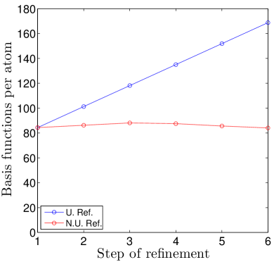
This strategy may not yield an efficient distribution of basis functions if the initial distribution 𝒥1subscript𝒥1\mathcal{J}_{1} contains too few basis functions to reasonably resolve the system, nor is it intended to do so. In this case, the local estimator may not be effective at the first step, which could lead to erratic estimates of local error. It is not necessarily the case that the total number of basis functions will increase as the basis is refined - as we will demonstrate in Section 4, the total number of basis functions may very well decrease through the refinement process - so all available resources may be used to make the initial calculation. Rather, the refinement process redistributes basis functions to achieve higher accuracy at a minimum cost by adding basis functions to under-resolved elements and removing basis functions from over-resolved elements.

  Input: ϵminsubscriptitalic-ϵ\epsilon_{\min}, ϵmaxsubscriptitalic-ϵ\epsilon_{\max}, initial distribution of basis functions 𝒥1={JK,1}K𝒯subscript𝒥1subscriptsubscript𝐽𝐾1𝐾𝒯\mathcal{J}_{1}=\{J_{K,1}\}_{K\in\mathcal{T}}, n𝑛n, bstepsubscript𝑏stepb_{\text{step}}
  Output: Refined distribution of basis functions 𝒥nsubscript𝒥𝑛\mathcal{J}_{n}, and physical quantities such as electron density ρ𝜌\rho
  for 1jn11𝑗𝑛11\leq j\leq n-1 do
     Compute a set of eigenpairs {(εi,𝒥j,ui,𝒥j)}i=1Nsuperscriptsubscriptsubscript𝜀𝑖subscript𝒥𝑗subscript𝑢𝑖subscript𝒥𝑗𝑖1𝑁\{(\varepsilon_{i,\mathcal{J}_{j}},u_{i,\mathcal{J}_{j}})\}_{i=1}^{N} based on the ALB approach
     for K𝒯𝐾𝒯K\in\mathcal{T} do
        Compute ηK2superscriptsubscript𝜂𝐾2\eta_{K}^{2}
        if ηK2<ϵminsuperscriptsubscript𝜂𝐾2subscriptitalic-ϵ\eta_{K}^{2}<\epsilon_{\min} then
           Update JK,j+1JK,jbstepsubscript𝐽𝐾𝑗1subscript𝐽𝐾𝑗subscript𝑏stepJ_{K,j+1}\leftarrow J_{K,j}-b_{\text{step}}
        else if ηK2>ϵmaxsuperscriptsubscript𝜂𝐾2subscriptitalic-ϵ\eta_{K}^{2}>\epsilon_{\max} then
           Update JK,j+1JK,j+bstepsubscript𝐽𝐾𝑗1subscript𝐽𝐾𝑗subscript𝑏stepJ_{K,j+1}\leftarrow J_{K,j}+b_{\text{step}}
        else
           Update JK,j+1JK,jsubscript𝐽𝐾𝑗1subscript𝐽𝐾𝑗J_{K,j+1}\leftarrow J_{K,j}
        end if
     end for
  end for
  Compute and output physical quantities (such as ρ𝜌\rho) using 𝒥nsubscript𝒥𝑛\mathcal{J}_{n}
Algorithm 1 Non-uniform basis refinement procedure.

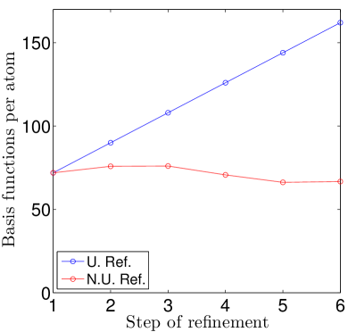
Let us contrast the non-uniform refinement procedure with a uniform refinement procedure, in which some number bstepsubscript𝑏stepb_{\text{step}} of basis functions are added to every element for each of n𝑛n steps. If we carry out uniform and non-uniform refinement with the same choices of bstepsubscript𝑏stepb_{\text{step}} and n𝑛n, and the same initial distribution of basis functions 𝒥1subscript𝒥1\mathcal{J}_{1}, we can compare the accuracy and total number of basis functions used at each step of the two refinement processes. The maximum possible number of basis functions assigned to any element on a given step of the non-uniform refinement scheme will always be equal to the number of basis functions in all elements on the same step of the uniform refinement scheme, but the minimum number of basis functions assigned to any element may be as little as zero. Therefore, the error on a given step of the uniform refinement scheme will always be less than or equal to that on the corresponding step of the non-uniform refinement scheme, up to small numerical errors incurred during the course of the solution process. We may then ask how much less is the error obtained from uniform refinement than from non-uniform refinement, and how many more basis functions are used to make it so. This is the criterion by which the non-uniform refinement scheme will be judged against a uniform refinement scheme for the calculations presented in Section 4.

4 Numerical results for Kohn-Sham density functional theory calculations

In this section we present numerical results which demonstrate that the global estimator is effective in predicting the error of the total energy, and that the local estimator may be used to guide efficient non-uniform local basis refinement. Although the theoretical part of the paper only aims at developing an a posteriori error estimator for linear eigenvalue problems, we apply the estimator to solve the nonlinear Kohn-Sham equations. All numerical results are performed with converged self-consistent field iterations. They properly take into account the nonlinearity of the Kohn-Sham equations. We test the refinement strategy for Kohn-Sham density functional theory calculations on two example systems. The first is an aluminum surface with a large vacuum region, and the second is a single layer of graphene oxide in water. These systems are highly inhomogeneous and therefore serve as good benchmark examples of non-uniform adaptive local basis refinement.

The evaluation of the a posteriori error estimator and the refinement strategy are implemented in the Discontinuous Galerkin Density Functional Theory (DGDFT) software. The energies and atomic forces are directly compared with the results obtained from ABINIT [20] using the same atomic configuration. We note that although the analysis in Section 3 is given for the linear eigenvalue problem, in all the numerical examples we solve the nonlinear eigenvalue problem as is required for KSDFT calculations. The results presented for both DGDFT and for ABINIT calculations have achieved convergence in the self-consistent field (SCF) iteration. In both the DGDFT and the ABINIT calculations, we use the local density approximation (LDA) [8, 34] for the exchange-correlation functional, and the Hartwigsen-Goedecker-Hutter (HGH) pseudopotential [21] with the local and non-local pseudopotential fully implemented in the real space [32]. All quantities are reported in atomic units (au). All calculations are carried out on the Edison system maintained at the National Energy Research Scientific Computing Center (NERSC). Each compute node on Edison has 242424 Intel “Ivy Bridge” cores (2.42.42.4 GHz) with 646464 gigabytes (GB) of memory.

As a first attempt we use the choice of parameters in Eq. (3.42) to define the a posteriori error estimator. We define hKsubscript𝐾h_{K} to be the diameter of the element K𝐾K, and we reinterpret pKsubscript𝑝𝐾p_{K} to be the number of ALBs rather than the polynomial degree in each element K𝐾K. Our results indicate that for the examples studied, the global estimator η2=K𝒯ηK2superscript𝜂2subscript𝐾𝒯superscriptsubscript𝜂𝐾2\eta^{2}=\sum_{K\in\mathcal{T}}\eta_{K}^{2} is numerically effective in predicting the error of the total energy within a relatively small constant factor, and that the local estimator ηK2superscriptsubscript𝜂𝐾2\eta_{K}^{2} is numerically effective in predicting the error in each element K𝐾K of the computed electron density ρ𝜌\rho. As a result, the non-uniform basis refinement strategy yields efficient distributions of local basis functions across the elements for these examples. Replacing a uniform refinement scheme with a non-uniform refinement scheme incurs very little loss in accuracy, but allows the use of a much smaller basis and hence gives significant computational savings.

4.1 Quasi-2D aluminum surface

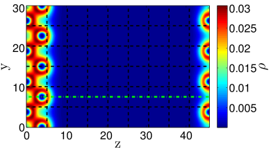
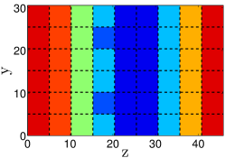
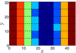
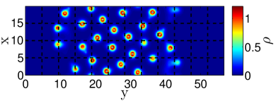
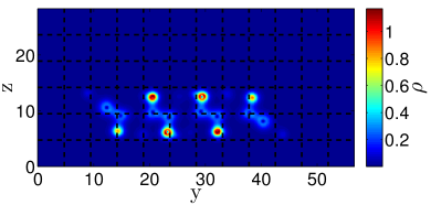
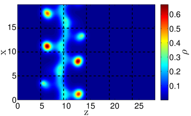
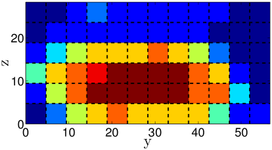
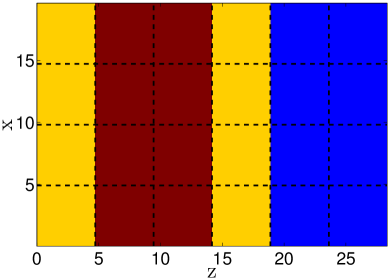
The first example is a quasi-2D aluminum surface with a large vacuum region. The periodic domain contains 16 aluminum atoms arranged in a row, and a large vacuum region. The size of the supercell is approximately 7.657.657.65 au, 30.6130.6130.61 au and 45.9245.9245.92 au along the x,y,𝑥𝑦x,y, and z𝑧z directions, respectively. The computational domain is partitioned into a 1×6×91691\times 6\times 9 grid of elements. The size of the extended element is always 333 times the size of the element along each direction, unless there is only one element and in this case the size of the extended element is the same as the size of the element. One slice of the electron density ρ𝜌\rho in the yz𝑦𝑧y-z plane is shown in Fig. 1a, and another in the xy𝑥𝑦x-y plane in Fig. 1b. The black dashed lines indicate the partition of the elements. In DGDFT, a uniform grid is used to represent quantities such as the electron density and potential in the global domain, with 707070, 276276276, and 414414414 grid points along the x𝑥x, y𝑦y, and z𝑧z directions, respectively. A Legendre-Gauss-Lobatto (LGL) grid is used inside each element to construct the DG Hamiltonian matrix, and the number of LGL grid points inside each element is 140140140, 929292, and 929292 along the x𝑥x, y𝑦y, and z𝑧z directions, respectively.

Refer to caption

(a) Fixed x = 3.8267

Refer to caption

(b) Fixed z = 0
Figure 1: Electron density ρ𝜌\rho in the (a) yz𝑦𝑧y-z plane and in the (b) xy𝑥𝑦x-y plane. The partition of the global domain into 1×6×91691\times 6\times 9 elements is indicated by black dashed lines.

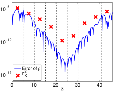
Fig. 2 shows the pointwise error of the electron density corresponding to the slice shown in Fig. 1a, with 50 adaptive local basis functions used in each element. The error of the density ρ𝜌\rho is highly non-uniform across different elements; the error in the elements which contain atoms can be more than 555 orders of magnitude larger than that in elements in the vacuum region.

Fig. 3a shows the slice of electron density along y=7.6534𝑦7.6534y=7.6534 as indicated by the green dash-dotted line in Fig. 1a. Fig. 3b shows the error of the electron density, along with the values of the local estimator ηK2superscriptsubscript𝜂𝐾2\eta_{K}^{2} in each of the elements K𝐾K through which the slice passes. We observe that the local estimator provides an upper bound for the local error of the electron density, and can be used to indicate the relative contributions of the various elements to this error in the adaptive refinement procedure.
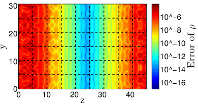
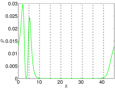
Refer to caption
Figure 2: The pointwise error of the electron density ρ𝜌\rho (in log scale) for the slice shown in Figure 1a when 50 adaptive local basis functions are used in each element. The error in different elements differ by several orders of magnitude, which indicates that non-uniform distribution of basis functions may be used to generate more efficient electronic structure calculations for this system. The error is computed by comparing with the DGDFT result an accurate calculation obtained using the software package ABINIT.

Refer to caption

(a) Electron density

Refer to caption

(b) Pointwise error of slice and local estimator
Figure 3: (a) One-dimensional slice of the electron density indicated by the green dash-dotted line in Fig. 1a at y=7.6534𝑦7.6534y=7.6534. (b) The error of the electron density along with the local estimator ηK2superscriptsubscript𝜂𝐾2\eta_{K}^{2} along the one dimensional slice, demonstrating the effectiveness of the local estimator at predicting the local error of ρ𝜌\rho.

Let us next compare the accuracy and efficiency of uniform and non-uniform basis refinement schemes for this system. In both schemes, we begin with 25 adaptive local basis functions in all elements on the first step. We specify the basis refinement step size bstep=5subscript𝑏step5b_{\text{step}}=5 and the number of steps n=6𝑛6n=6. In the uniform refinement scheme, we simply add bstep=5subscript𝑏step5b_{\text{step}}=5 basis functions to each element on each step. The non-uniform refinement scheme follows Algorithm 1 with ϵmax=5×10⁶subscriptitalic-ϵ5superscript106\epsilon_{\max}=5\times 10^{-6} and ϵmin=5×10⁷subscriptitalic-ϵ5superscript107\epsilon_{\min}=5\times 10^{-7}.

We first examine the distribution of basis functions produced by the non-uniform refinement scheme, shown for all steps in Figure 4. The scheme eventually places more basis functions in elements for which a uniform distribution of basis functions produces larger pointwise errors. This becomes clear when comparing Figures 4 and 2, the latter of which gives the pointwise error in the density for the last step of the uniform refinement scheme. Indeed, the non-uniform scheme allocates zero basis functions to the elements which contain the smallest pointwise errors in the uniform scheme, and the maximum possible number of basis functions to the elements which contain the largest pointwise errors in the uniform scheme.
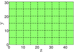
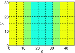
Refer to caption
(a) Step 1
Refer to caption
(b) Step 2
Refer to caption
(c) Step 3
Refer to caption
(d) Step 4
Refer to caption
(e) Step 5
Refer to caption
(f) Step 6
Refer to caption
(g)
Figure 4: Distribution of adaptive local basis functions in six steps of non-uniform refinement for aluminum system. The final distribution mirrors the pointwise errors shown in Fig. 2.

At the last step of refinement, the non-uniform refinement scheme uses half as many basis functions per atom as the uniform refinement scheme, as shown in Fig. 5c. These savings are obtained without sacrificing accuracy. Fig. 5a show that the error per atom of the total energy is nearly equal using both methods, despite the large difference in the number of basis functions used. We also measure the accuracy of the atomic force, which is given by the derivative of the energy with respect to the atomic positions. The atomic force is used in various applications including geometry optimization and molecular dynamics. We measure both the maximum and the average Euclidean error of the atomic forces among all atoms. Fig. 5b shows that both accuracy measurements are nearly the same using uniform and non-uniform refinement. We therefore see that non-uniform refinement significantly improves the efficiency of the adaptive local basis functions by simply redistributing basis functions according to the predictions of the local estimator, without sacrificing accuracy.
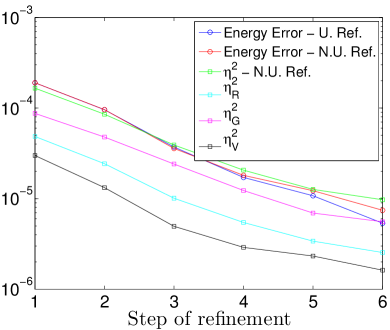
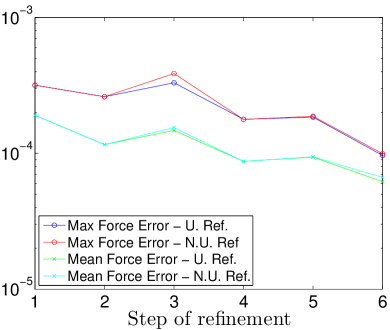
Refer to caption
(a) Error per atom of total energy (Hartree/atom) for uniform refinement (U. Ref.) and non-uniform refinement (N.U. Ref), along with the global estimator. We also show the individual terms of the estimator summed over all elements K𝒯𝐾𝒯K\in\mathcal{T}; the residual ηR2superscriptsubscript𝜂𝑅2\eta_{R}^{2}, the discontinuity of the gradient ηG2superscriptsubscript𝜂𝐺2\eta_{G}^{2}, and the discontinuity of the function values ηV2superscriptsubscript𝜂𝑉2\eta_{V}^{2}.
Refer to caption
(b) Error of atomic force (au) for uniform and non-uniform refinement.
Refer to caption
(c) Number of basis functions per atom for uniform and non-uniform refinement.
Figure 5: Accuracy and savings for aluminum system calculations. The non-uniform refinement scheme produces results which are nearly as accurate as those produced by the uniform refinement scheme, using only half as many basis functions.

We lastly demonstrate that the use of non-uniformly distributed adaptive local basis functions gives significant savings over the use of planewave basis functions as in ABINIT. The number of basis functions in planewave-based electronic structure calculations is usually denoted by the kinetic energy cutoff (Ecutsubscript𝐸cutE_{\mathrm{cut}}). In atomic units, the relation between the total number Npwsubscript𝑁pwN_{\mathrm{pw}} of basis functions used in a planewave calculation and Ecutsubscript𝐸cutE_{\mathrm{cut}} is approximately (depending on adjustments to the number of grid points for performance improvements) [30]

Npw=(2Ecutπ)3Vol,subscript𝑁pwsuperscript2subscript𝐸cut𝜋3VolN_{\mathrm{pw}}=\left(\frac{\sqrt{2E_{\mathrm{cut}}}}{\pi}\right)^{3}\mathrm{Vol}, (4.65)

where VolVol\mathrm{Vol} is the volume of the computational domain.

Fig. 6 plots the number of basis functions per atom against the error per atom of the total energy using the planewave basis set obtained from ABINIT, a uniform distribution of adaptive local basis functions obtained from DGDFT, and a non-uniform distribution of adaptive local basis functions obtained from DGDFT. We observe that DGDFT calculations use many fewer basis functions than ABINIT calculations to achieve similar error. For example, to achieve an error of the total energy on the order of 106superscript10610^{-6} Hartree per atom, ABINIT requires around 10,0001000010,000 planewave basis functions per atom, whereas DGDFT requires approximately 848484 adaptive local basis functions per atom when non-uniform basis refinement is used.
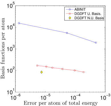
Refer to caption
Figure 6: Number of basis functions used to achieve a given error of the total energy for the aluminum example. Non-uniform adaptive local basis sets obtained from DGDFT are approximately two orders of magnitude smaller than planewave basis sets obtained from ABINIT for similar error.

4.2 Graphene oxide

We next consider a layer of graphene oxide in water, consisting of 160160160 atoms, with the atomic configuration shown in Fig. 7. The size of the supercell is 19.6319.6319.63 au, 56.6956.6956.69 au and 28.3528.3528.35 au along the x,y,𝑥𝑦x,y, and z𝑧z directions, respectively. The computational domain is partitioned into a 4×12×641264\times 12\times 6 grid of elements. As in the case of the aluminum system, a uniform grid is used to represent quantities such as the electron density and potential in the global domain in DGDFT, with 160160160, 456456456, and 228228228 grid points along the x𝑥x, y𝑦y, and z𝑧z directions, respectively. A Legendre-Gauss-Lobatto (LGL) grid is used inside each element to construct the DG Hamiltonian matrix, and the number of LGL grid points inside each element is 808080, 767676, and 767676 along the x𝑥x, y𝑦y, and z𝑧z directions, respectively. Fig. 8 shows slices of the density across various planes.

We perform both uniform and non-uniform refinement of the basis functions. We begin with a uniform distribution of 40 basis functions in each element for both schemes. The basis refinement step size is set at bstep=10subscript𝑏step10b_{\text{step}}=10 and the number of refinement steps at n=6𝑛6n=6. For the non-uniform refinement scheme, we use ϵmax=104subscriptitalic-ϵ𝑚𝑎𝑥superscript104\epsilon_{max}=10^{-4} and ϵmin=106subscriptitalic-ϵ𝑚𝑖𝑛superscript106\epsilon_{min}=10^{-6}. Fig. 9 shows the final distributions of adaptive local basis functions generated by the non-uniform refinement process in the elements containing the slices shown in Fig. 8. The distribution of adaptive local basis functions corresponds well to the highly inhomogeneous electron density of the system.
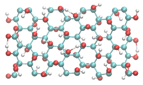
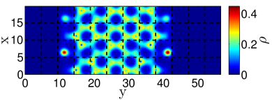
Refer to caption
Figure 7: Atomic configuration of a single layer of graphene oxide in water with 160160160 atoms.
Refer to caption
(a) Fixed z = 9.2975
Refer to caption
(b) Fixed z = 12.3966

Refer to caption

(c) Fixed x = 10.9079

Refer to caption

(d) Fixed y = 24.0205
Figure 8: Two-dimensional slices of electron density for graphene oxide system, with 4×12×641264\times 12\times 6 grid used in DGDFT calculations indicated by black dashed lines.
Refer to caption
(a) Fixed z = 9.2975
Refer to caption
(b) Fixed z = 12.3966

Refer to caption

(c) Fixed x = 10.9079

Refer to caption

(d) Fixed y = 24.0205
Refer to caption
(e)
Figure 9: Distributions of adaptive local basis functions at the last step of non-uniform refinement in the elements containing the slices shown in Figure 8. The distribution of basis functions closely reflects the density.

Fig. 10 demonstrates the accuracy and efficiency of the non-uniform refinement procedure for the graphene oxide calculation. Fig. 10a shows that the difference in the error of the total energy per atom for the two refinement schemes is very small, and that the global estimator is highly effective in capturing the error of the total energy. The maximum and average errors of the atomic forces among all the atoms are given in Fig. 10b for the uniform and non-uniform refinement schemes, which again give similar accuracy. Fig. 10c shows that by the final step of refinement, the uniform refinement scheme uses nearly 2.5 times as many basis functions as the non-uniform refinement scheme. Furthermore, the non-uniform refinement scheme uses fewer basis functions at the final step than it does at the first step, though the error is four orders of magnitude lower.
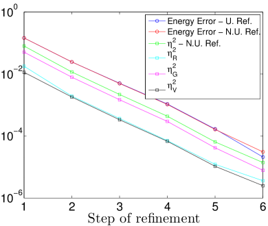
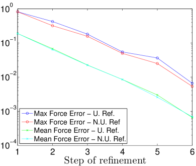
Refer to caption
(a) Error per atom of total energy (Hartree/atom) for uniform refinement (U. Ref.) and non-uniform refinement (N.U. Ref), along with the global estimator. We also show the individual terms of the estimator summed over all elements K𝒯𝐾𝒯K\in\mathcal{T}; the residual ηR2superscriptsubscript𝜂𝑅2\eta_{R}^{2}, the discontinuity of the gradient ηG2superscriptsubscript𝜂𝐺2\eta_{G}^{2}, and the discontinuity of the function values ηV2superscriptsubscript𝜂𝑉2\eta_{V}^{2}.
Refer to caption
(b) Error of atomic force (au) for uniform and non-uniform refinement.
Refer to caption
(c) Number of basis functions per atom for uniform and non-uniform refinement.
Figure 10: Accuracy and savings for graphene oxide system calculations. As in the aluminum case, the non-uniform refinement scheme is nearly as accurate and more efficient than the uniform scheme, and the global estimator is asymptotically effective.

Another perspective on the effectiveness of the non-uniform refinement strategy is given in Fig. 11, in which we plot the quintile values of the local estimator across all elements at each step of uniform and non-uniform refinement, along with the error thresholds ϵmaxsubscriptitalic-ϵ\epsilon_{\max} and ϵminsubscriptitalic-ϵ\epsilon_{\min}. In the uniform refinement scheme, both under and over-resolved elements become further refined at each step. In the non-uniform refinement scheme, only the under-resolved elements are further refined; the over-resolved elements are instead made less refined at each step, thus recovering inefficiently-allocated resources. The dominant sources of error are similar in both cases, so very little loss in accuracy is incurred by using a non-uniform basis refinement scheme.
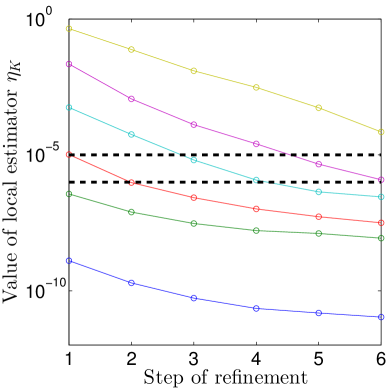
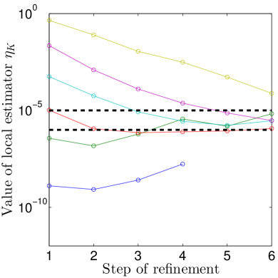
Refer to caption
(a) Uniform refinement
Refer to caption
(b) Non-uniform refinement
Figure 11: Quintile values of local estimator for uniform and non-uniform basis refinement, along with ϵmaxsubscriptitalic-ϵ\epsilon_{\max} and ϵminsubscriptitalic-ϵ\epsilon_{\min}. The dominant local errors are roughly the same in both elements, but the non-uniform refinement scheme produces savings in the elements with small local error. Note that the minimum value of the local estimator across all elements becomes 00 by the fifth step of non-uniform refinement.

Fig. 12 compares the number of planewave basis functions used by ABINIT with the number of adaptive local basis functions used by DGDFT to achieve similar error for the graphene oxide example. We observe, for example, that to achieve an error of the total energy on the order of 105superscript10510^{-5} Hartree per atom, ABINIT requires around 35,0003500035,000 planewave basis functions per atom, whereas DGDFT requires approximately 676767 adaptive local basis functions per atom when non-uniform basis refinement is used.
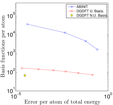
Refer to caption
Figure 12: Number of basis functions used to achieve a given error of the total energy for the GO example. Non-uniform adaptive local basis sets obtained from DGDFT are approximately three orders of magnitude smaller than planewave basis sets obtained from ABINIT for similar error.

5 Conclusion and future work

In this paper we develop residual-based a posteriori local error estimates for solving KSDFT using adaptive local basis functions in a discontinuous Galerkin framework. Compared with standard hp𝑝hp-refinement, the major difficulty in carrying out the analysis is that little is known about the analytical properties of the adaptive local basis functions. We therefore effectively need to perform an a posteriori error analysis for general non-polynomial basis functions. In order to proceed we postulate a set of assumptions on the basis set under which we are able to prove that the a posteriori error estimator is an upper bound for the errors of both eigenvalues and eigenvectors, up to terms which are of higher order in the context of standard hp𝑝hp-refinement. We acknowledge that there is still difficulty in verifying the assumptions for a specific non-polynomial basis set such as the ALBs. We plan to carry out a numerical verification of the assumptions for the adaptive local basis functions in the future. The hope is that such a study can illuminate the approximation properties of the ALB sets from an analytic point of view, and also inform the a priori error analysis.

From a practical point of view, the results given by the local error estimator used in DGDFT mimic the hp𝑝hp-refinement results. As a first attempt we reinterpret p𝑝p as the number of adaptive local basis functions used in each element. We consider this only as a starting point for the study, but nevertheless, the numerical results show that the approach of a posteriori error estimates is promising for KSDFT studies. We demonstrate the practical use of the a posteriori error estimator for three-dimensional KSDFT calculations for quasi-2D aluminum surfaces and a single layer graphene oxide system in water. Besides the systems with a vacuum region, we also plan to use the non-uniform refinement strategy to study systems with defects and dislocations. In these cases, the electron density and the magnitude of the estimator may not vary as much as in the case of a large vacuum region.

Besides the adaptive refinement, another important application of a posteriori error estimation is to capture the error due to the finite dimensional approximation of physical quantities such as total energies without performing a more refined calculation, which can be prohibitively expensive in practical KSDFT calculations. The error of the total energy is directly related to the error of eigenvalues. However, this objective requires a much more precise estimator than is used in the current formulation, and this will be our future work.

Acknowledgments

This work was partially supported by the Science Undergraduate Laboratory Internship (SULI) program of Lawrence Berkeley National Laboratory (J. K.), by the Laboratory Directed Research and Development Program of Lawrence Berkeley National Laboratory under the U.S. Department of Energy contract number DE-AC02-05CH11231, and by the Scientific Discovery through Advanced Computing (SciDAC) program funded by U.S. Department of Energy, Office of Science, Advanced Scientific Computing Research and Basic Energy Sciences (L. L. and C. Y.). We are grateful to Roberto Car and Limin Liu for providing the atomic configuration of the graphene oxide in water. We would also like to thank Eric Cancès, Yvon Maday and Benjamin Stamm for helpful discussions.

Appendix A Details for proving Theorem 3.3 and 3.7

Lemma A.1.

Let ui,𝒥rsuperscriptsubscript𝑢𝑖𝒥𝑟u_{i,\mathcal{J}}^{r} be defined as in Eq. (3.48), then

ui,𝒥rE,𝒯ηi.less-than-or-similar-tosubscriptdelimited-∥∥superscriptsubscript𝑢𝑖𝒥𝑟𝐸𝒯subscript𝜂𝑖\left\lVert u_{i,\mathcal{J}}^{r}\right\rVert_{E,\mathcal{T}}\lesssim\eta_{i}. (1.66)
Proof A.2.

Using Eq. (3.35)

K𝒯ui,𝒥rK2F𝒮γ2(JF)α2(JF)[[ui,𝒥]]F2K𝒯ηi,VK2ηi2.less-than-or-similar-tosubscript𝐾𝒯subscriptsuperscriptdelimited-∥∥superscriptsubscript𝑢𝑖𝒥𝑟2𝐾subscript𝐹𝒮subscript𝛾2subscript𝐽𝐹superscript𝛼2subscript𝐽𝐹subscriptsuperscriptdelimited-∥∥delimited-[]delimited-[]subscript𝑢𝑖𝒥2𝐹less-than-or-similar-tosubscript𝐾𝒯superscriptsubscript𝜂𝑖subscript𝑉𝐾2superscriptsubscript𝜂𝑖2\sum_{K\in\mathcal{T}}\left\lVert\nabla u_{i,\mathcal{J}}^{r}\right\rVert^{2}_{K}\lesssim\sum_{F\in\mathcal{S}}\gamma_{2}(J_{F})\alpha^{2}(J_{F})\left\lVert\big{[}\big{[}u_{i,\mathcal{J}}\big{]}\big{]}\right\rVert^{2}_{F}\lesssim\sum_{K\in\mathcal{T}}\eta_{i,V_{K}}^{2}\leq\eta_{i}^{2}. (1.67)

Using Eq. (3.34),

F𝒮α(JF)[[ui,𝒥]]F2F𝒮γ2(JF)α2(JF)[[ui,𝒥]]F2K𝒯ηi,VK2ηi2.less-than-or-similar-tosubscript𝐹𝒮𝛼subscript𝐽𝐹subscriptsuperscriptdelimited-∥∥delimited-[]delimited-[]subscript𝑢𝑖𝒥2𝐹subscript𝐹𝒮subscript𝛾2subscript𝐽𝐹superscript𝛼2subscript𝐽𝐹subscriptsuperscriptdelimited-∥∥delimited-[]delimited-[]subscript𝑢𝑖𝒥2𝐹less-than-or-similar-tosubscript𝐾𝒯superscriptsubscript𝜂𝑖subscript𝑉𝐾2superscriptsubscript𝜂𝑖2\sum_{F\in\mathcal{S}}\alpha(J_{F})\left\lVert\big{[}\big{[}u_{i,\mathcal{J}}\big{]}\big{]}\right\rVert^{2}_{F}\lesssim\sum_{F\in\mathcal{S}}\gamma_{2}(J_{F})\alpha^{2}(J_{F})\left\lVert\big{[}\big{[}u_{i,\mathcal{J}}\big{]}\big{]}\right\rVert^{2}_{F}\lesssim\sum_{K\in\mathcal{T}}\eta_{i,V_{K}}^{2}\leq\eta_{i}^{2}. (1.68)

Then Lemma 1.66 follows directly from the definition of the energy norm (3.44).

Definition A.3 (Split of A𝒥subscript𝐴𝒥A_{\mathcal{J}}).

The bilinear form A𝒥subscript𝐴𝒥A_{\mathcal{J}} in Eq. (2.24) can be split into two parts

A𝒥(u,v)=D𝒥(u,v)+K𝒥(u,v).subscript𝐴𝒥𝑢𝑣subscript𝐷𝒥𝑢𝑣subscript𝐾𝒥𝑢𝑣A_{\mathcal{J}}(u,v)=D_{\mathcal{J}}(u,v)+K_{\mathcal{J}}(u,v). (1.69)

Here

D𝒥(u,v)=12u,v𝒯+F𝒮α(JF)[[u]],[[v]]F,subscript𝐷𝒥𝑢𝑣12subscript𝑢𝑣𝒯subscript𝐹𝒮𝛼subscript𝐽𝐹subscriptdelimited-[]delimited-[]𝑢delimited-[]delimited-[]𝑣𝐹D_{\mathcal{J}}(u,v)=\frac{1}{2}\left\langle\nabla u,\nabla v\right\rangle_{\mathcal{T}}+\sum_{F\in\mathcal{S}}\alpha(J_{F})\left\langle\big{[}\big{[}u\big{]}\big{]},\big{[}\big{[}v\big{]}\big{]}\right\rangle_{F}, (1.70)

and

K𝒥(u,v)=12{{u}},[[v]]𝒮12{{v}},[[u]]𝒮.subscript𝐾𝒥𝑢𝑣12subscript𝑢delimited-[]delimited-[]𝑣𝒮12subscript𝑣delimited-[]delimited-[]𝑢𝒮K_{\mathcal{J}}(u,v)=-\frac{1}{2}\left\langle\big{\{}\big{\{}\nabla u\big{\}}\big{\}},\big{[}\big{[}v\big{]}\big{]}\right\rangle_{\mathcal{S}}-\frac{1}{2}\left\langle\big{\{}\big{\{}\nabla v\big{\}}\big{\}},\big{[}\big{[}u\big{]}\big{]}\right\rangle_{\mathcal{S}}. (1.71)

Formally, it is clear that

A(u,v)=D𝒥(u,v),u,vHπ1(Ω).formulae-sequence𝐴𝑢𝑣subscript𝐷𝒥𝑢𝑣for-all𝑢𝑣subscriptsuperscript𝐻1𝜋ΩA(u,v)=D_{\mathcal{J}}(u,v),\quad\forall u,v\in H^{1}_{\pi}(\Omega). (1.72)
Lemma A.4.

If Assumption 3.1 holds, let (εi,𝒥,ui,𝒥)subscript𝜀𝑖𝒥subscript𝑢𝑖𝒥(\varepsilon_{i,\mathcal{J}},u_{i,\mathcal{J}}) be a computed eigenpair corresponding to (2.23), and (εi,ui)subscript𝜀𝑖subscript𝑢𝑖(\varepsilon_{i},u_{i}) an eigenpair corresponding to (2.28). For any vHπ1(Ω)𝑣subscriptsuperscript𝐻1𝜋Ωv\in H^{1}_{\pi}(\Omega), let v𝒥𝒱𝒥(𝒯)subscript𝑣𝒥subscript𝒱𝒥𝒯v_{\mathcal{J}}\in\mathcal{V}_{\mathcal{J}}(\mathcal{T}) satisfy (3.31) and (3.32). Then we have

εiuiVeffui,vv𝒥𝒯D𝒥(ui,𝒥,vv𝒥)+K𝒥(ui,𝒥,v𝒥)(ηi+γ1,𝒥ξi)vE,𝒯.less-than-or-similar-tosubscriptsubscript𝜀𝑖subscript𝑢𝑖subscript𝑉effsubscript𝑢𝑖𝑣subscript𝑣𝒥𝒯subscript𝐷𝒥subscript𝑢𝑖𝒥𝑣subscript𝑣𝒥subscript𝐾𝒥subscript𝑢𝑖𝒥subscript𝑣𝒥subscript𝜂𝑖subscript𝛾1𝒥subscript𝜉𝑖subscriptdelimited-∥∥𝑣𝐸𝒯\begin{split}&\left\langle\varepsilon_{i}u_{i}-V_{\mathrm{eff}}u_{i},v-v_{\mathcal{J}}\right\rangle_{\mathcal{T}}-D_{\mathcal{J}}(u_{i,\mathcal{J}},v-v_{\mathcal{J}})+K_{\mathcal{J}}(u_{i,\mathcal{J}},v_{\mathcal{J}})\\ &~{}~{}~{}\lesssim\left(\eta_{i}+\sqrt{\gamma_{1,\mathcal{J}}}\xi_{i}\right)\left\lVert v\right\rVert_{E,\mathcal{T}}.\end{split} (1.73)
Proof A.5.

For brevity, set

T=εiuiVeffui,vv𝒥𝒯D𝒥(ui,𝒥,vv𝒥)+K𝒥(ui,𝒥,v𝒥)𝑇subscriptsubscript𝜀𝑖subscript𝑢𝑖subscript𝑉effsubscript𝑢𝑖𝑣subscript𝑣𝒥𝒯subscript𝐷𝒥subscript𝑢𝑖𝒥𝑣subscript𝑣𝒥subscript𝐾𝒥subscript𝑢𝑖𝒥subscript𝑣𝒥T=\left\langle\varepsilon_{i}u_{i}-V_{\mathrm{eff}}u_{i},v-v_{\mathcal{J}}\right\rangle_{\mathcal{T}}-D_{\mathcal{J}}(u_{i,\mathcal{J}},v-v_{\mathcal{J}})+K_{\mathcal{J}}(u_{i,\mathcal{J}},v_{\mathcal{J}}) (1.74)

Integrating by parts gives

D𝒥(ui,𝒥,vv𝒥)=K𝒯12Δui,𝒥,vv𝒥K+F𝒮α(JF)[[ui,𝒥]],[[vv𝒥]]F+K𝒯12ui,𝒥𝐧K,vv𝒥Ksubscript𝐷𝒥subscript𝑢𝑖𝒥𝑣subscript𝑣𝒥subscript𝐾𝒯12subscriptΔsubscript𝑢𝑖𝒥𝑣subscript𝑣𝒥𝐾subscript𝐹𝒮𝛼subscript𝐽𝐹subscriptdelimited-[]delimited-[]subscript𝑢𝑖𝒥delimited-[]delimited-[]𝑣subscript𝑣𝒥𝐹subscript𝐾𝒯12subscriptsubscript𝑢𝑖𝒥subscript𝐧𝐾𝑣subscript𝑣𝒥𝐾\begin{split}D_{\mathcal{J}}(u_{i,\mathcal{J}},v-v_{\mathcal{J}})=&-\sum_{K\in\mathcal{T}}\frac{1}{2}\left\langle\Delta u_{i,\mathcal{J}},v-v_{\mathcal{J}}\right\rangle_{K}+\sum_{F\in\mathcal{S}}\alpha(J_{F})\left\langle\big{[}\big{[}u_{i,\mathcal{J}}\big{]}\big{]},\big{[}\big{[}v-v_{\mathcal{J}}\big{]}\big{]}\right\rangle_{F}\\ &+\sum_{K\in\mathcal{T}}\frac{1}{2}\left\langle\nabla u_{i,\mathcal{J}}\cdot\mathbf{n}_{K},v-v_{\mathcal{J}}\right\rangle_{\partial K}\end{split} (1.75)

Using the identity

K𝒯ui,𝒥𝐧K,vv𝒥K=F𝒮{{ui,𝒥}},[[vv𝒥]]F+F𝒮[[ui,𝒥]],{{vv𝒥}}F,subscript𝐾𝒯subscriptsubscript𝑢𝑖𝒥subscript𝐧𝐾𝑣subscript𝑣𝒥𝐾subscript𝐹𝒮subscriptsubscript𝑢𝑖𝒥delimited-[]delimited-[]𝑣subscript𝑣𝒥𝐹subscript𝐹𝒮subscriptdelimited-[]delimited-[]subscript𝑢𝑖𝒥𝑣subscript𝑣𝒥𝐹\begin{split}\sum_{K\in\mathcal{T}}\left\langle\nabla u_{i,\mathcal{J}}\cdot\mathbf{n}_{K},v-v_{\mathcal{J}}\right\rangle_{\partial K}&=\sum_{F\in\mathcal{S}}\left\langle\big{\{}\big{\{}\nabla u_{i,\mathcal{J}}\big{\}}\big{\}},\big{[}\big{[}v-v_{\mathcal{J}}\big{]}\big{]}\right\rangle_{F}\\ &+\sum_{F\in\mathcal{S}}\left\langle\big{[}\big{[}\nabla u_{i,\mathcal{J}}\big{]}\big{]},\big{\{}\big{\{}v-v_{\mathcal{J}}\big{\}}\big{\}}\right\rangle_{F},\end{split} (1.76)

we have

T=K𝒯εiui+12Δui,𝒥Veffui,vv𝒥KF𝒮α(JF)[[ui,𝒥]],[[vv𝒥]]FF𝒮12{{ui,𝒥}},[[vv𝒥]]FF𝒮12[[ui,𝒥]],{{vv𝒥}}FF𝒮12{{ui,𝒥}},[[v𝒥]]FF𝒮12{{v𝒥}},[[ui,𝒥]]F=K𝒯εiui+12Δui,𝒥Veffui,vv𝒥KF𝒮α(JF)[[ui,𝒥]],[[vv𝒥]]FF𝒮12[[ui,𝒥]],{{vv𝒥}}FF𝒮12{{v𝒥}},[[ui,𝒥]]FT1+T2+T3+T4.𝑇subscript𝐾𝒯subscriptsubscript𝜀𝑖subscript𝑢𝑖12Δsubscript𝑢𝑖𝒥subscript𝑉effsubscript𝑢𝑖𝑣subscript𝑣𝒥𝐾subscript𝐹𝒮𝛼subscript𝐽𝐹subscriptdelimited-[]delimited-[]subscript𝑢𝑖𝒥delimited-[]delimited-[]𝑣subscript𝑣𝒥𝐹subscript𝐹𝒮12subscriptsubscript𝑢𝑖𝒥delimited-[]delimited-[]𝑣subscript𝑣𝒥𝐹subscript𝐹𝒮12subscriptdelimited-[]delimited-[]subscript𝑢𝑖𝒥𝑣subscript𝑣𝒥𝐹subscript𝐹𝒮12subscriptsubscript𝑢𝑖𝒥delimited-[]delimited-[]subscript𝑣𝒥𝐹subscript𝐹𝒮12subscriptsubscript𝑣𝒥delimited-[]delimited-[]subscript𝑢𝑖𝒥𝐹subscript𝐾𝒯subscriptsubscript𝜀𝑖subscript𝑢𝑖12Δsubscript𝑢𝑖𝒥subscript𝑉effsubscript𝑢𝑖𝑣subscript𝑣𝒥𝐾subscript𝐹𝒮𝛼subscript𝐽𝐹subscriptdelimited-[]delimited-[]subscript𝑢𝑖𝒥delimited-[]delimited-[]𝑣subscript𝑣𝒥𝐹subscript𝐹𝒮12subscriptdelimited-[]delimited-[]subscript𝑢𝑖𝒥𝑣subscript𝑣𝒥𝐹subscript𝐹𝒮12subscriptsubscript𝑣𝒥delimited-[]delimited-[]subscript𝑢𝑖𝒥𝐹subscript𝑇1subscript𝑇2subscript𝑇3subscript𝑇4\begin{split}T=&\sum_{K\in\mathcal{T}}\left\langle\varepsilon_{i}u_{i}+\frac{1}{2}\Delta u_{i,\mathcal{J}}-V_{\mathrm{eff}}u_{i},v-v_{\mathcal{J}}\right\rangle_{K}-\sum_{F\in\mathcal{S}}\alpha(J_{F})\left\langle\big{[}\big{[}u_{i,\mathcal{J}}\big{]}\big{]},\big{[}\big{[}v-v_{\mathcal{J}}\big{]}\big{]}\right\rangle_{F}\\ &-\sum_{F\in\mathcal{S}}\frac{1}{2}\left\langle\big{\{}\big{\{}\nabla u_{i,\mathcal{J}}\big{\}}\big{\}},\big{[}\big{[}v-v_{\mathcal{J}}\big{]}\big{]}\right\rangle_{F}-\sum_{F\in\mathcal{S}}\frac{1}{2}\left\langle\big{[}\big{[}\nabla u_{i,\mathcal{J}}\big{]}\big{]},\big{\{}\big{\{}v-v_{\mathcal{J}}\big{\}}\big{\}}\right\rangle_{F}\\ &-\sum_{F\in\mathcal{S}}\frac{1}{2}\left\langle\big{\{}\big{\{}\nabla u_{i,\mathcal{J}}\big{\}}\big{\}},\big{[}\big{[}v_{\mathcal{J}}\big{]}\big{]}\right\rangle_{F}-\sum_{F\in\mathcal{S}}\frac{1}{2}\left\langle\big{\{}\big{\{}\nabla v_{\mathcal{J}}\big{\}}\big{\}},\big{[}\big{[}u_{i,\mathcal{J}}\big{]}\big{]}\right\rangle_{F}\\ =&\sum_{K\in\mathcal{T}}\left\langle\varepsilon_{i}u_{i}+\frac{1}{2}\Delta u_{i,\mathcal{J}}-V_{\mathrm{eff}}u_{i},v-v_{\mathcal{J}}\right\rangle_{K}-\sum_{F\in\mathcal{S}}\alpha(J_{F})\left\langle\big{[}\big{[}u_{i,\mathcal{J}}\big{]}\big{]},\big{[}\big{[}v-v_{\mathcal{J}}\big{]}\big{]}\right\rangle_{F}\\ &-\sum_{F\in\mathcal{S}}\frac{1}{2}\left\langle\big{[}\big{[}\nabla u_{i,\mathcal{J}}\big{]}\big{]},\big{\{}\big{\{}v-v_{\mathcal{J}}\big{\}}\big{\}}\right\rangle_{F}-\sum_{F\in\mathcal{S}}\frac{1}{2}\left\langle\big{\{}\big{\{}\nabla v_{\mathcal{J}}\big{\}}\big{\}},\big{[}\big{[}u_{i,\mathcal{J}}\big{]}\big{]}\right\rangle_{F}\\ \equiv&T_{1}+T_{2}+T_{3}+T_{4}.\end{split} (1.77)

Here the definition of T1subscript𝑇1T_{1}, T2subscript𝑇2T_{2}, T3subscript𝑇3T_{3}, and T4subscript𝑇4T_{4} respects the order of the four terms in the second to last equality of Eq. (1.77). We shall proceed to prove that each T1,T2,T3,T4subscript𝑇1subscript𝑇2subscript𝑇3subscript𝑇4T_{1},T_{2},T_{3},T_{4} is bounded by the right hand side of Eq. (1.73).

For T1subscript𝑇1T_{1}, using the Cauchy-Schwarz inequality, we have

T1=K𝒯εi,𝒥ui,𝒥+12Δui,𝒥Veffui,𝒥,vv𝒥K+K𝒯εiuiεi,𝒥ui,𝒥Veffui+Veffui,𝒥,vv𝒥KK𝒯εi,𝒥ui,𝒥+12Δui,𝒥Veffui,𝒥Kvv𝒥K+K𝒯εiuiεi,𝒥ui,𝒥Veffui+Veffui,𝒥Kvv𝒥K=K𝒯(γ1(JK)εi,𝒥ui,𝒥+12Δui,𝒥Veffui,𝒥K)(1γ1(JK)vv𝒥K)+K𝒯(γ1(JK)εiuiεi,𝒥ui,𝒥Veffui+Veffui,𝒥K)(1γ1(JK)vv𝒥K)subscript𝑇1subscript𝐾𝒯subscriptsubscript𝜀𝑖𝒥subscript𝑢𝑖𝒥12Δsubscript𝑢𝑖𝒥subscript𝑉effsubscript𝑢𝑖𝒥𝑣subscript𝑣𝒥𝐾subscript𝐾𝒯subscriptsubscript𝜀𝑖subscript𝑢𝑖subscript𝜀𝑖𝒥subscript𝑢𝑖𝒥subscript𝑉effsubscript𝑢𝑖subscript𝑉effsubscript𝑢𝑖𝒥𝑣subscript𝑣𝒥𝐾subscript𝐾𝒯subscriptdelimited-∥∥subscript𝜀𝑖𝒥subscript𝑢𝑖𝒥12Δsubscript𝑢𝑖𝒥subscript𝑉effsubscript𝑢𝑖𝒥𝐾subscriptdelimited-∥∥𝑣subscript𝑣𝒥𝐾subscript𝐾𝒯subscriptdelimited-∥∥subscript𝜀𝑖subscript𝑢𝑖subscript𝜀𝑖𝒥subscript𝑢𝑖𝒥subscript𝑉effsubscript𝑢𝑖subscript𝑉effsubscript𝑢𝑖𝒥𝐾subscriptdelimited-∥∥𝑣subscript𝑣𝒥𝐾subscript𝐾𝒯subscript𝛾1subscript𝐽𝐾subscriptdelimited-∥∥subscript𝜀𝑖𝒥subscript𝑢𝑖𝒥12Δsubscript𝑢𝑖𝒥subscript𝑉effsubscript𝑢𝑖𝒥𝐾1subscript𝛾1subscript𝐽𝐾subscriptdelimited-∥∥𝑣subscript𝑣𝒥𝐾subscript𝐾𝒯subscript𝛾1subscript𝐽𝐾subscriptdelimited-∥∥subscript𝜀𝑖subscript𝑢𝑖subscript𝜀𝑖𝒥subscript𝑢𝑖𝒥subscript𝑉effsubscript𝑢𝑖subscript𝑉effsubscript𝑢𝑖𝒥𝐾1subscript𝛾1subscript𝐽𝐾subscriptdelimited-∥∥𝑣subscript𝑣𝒥𝐾\begin{split}T_{1}=&\sum_{K\in\mathcal{T}}\left\langle\varepsilon_{i,\mathcal{J}}u_{i,\mathcal{J}}+\frac{1}{2}\Delta u_{i,\mathcal{J}}-V_{\mathrm{eff}}u_{i,\mathcal{J}},v-v_{\mathcal{J}}\right\rangle_{K}\\ &+\sum_{K\in\mathcal{T}}\left\langle\varepsilon_{i}u_{i}-\varepsilon_{i,\mathcal{J}}u_{i,\mathcal{J}}-V_{\mathrm{eff}}u_{i}+V_{\mathrm{eff}}u_{i,\mathcal{J}},v-v_{\mathcal{J}}\right\rangle_{K}\\ \leq&\sum_{K\in\mathcal{T}}\left\lVert\varepsilon_{i,\mathcal{J}}u_{i,\mathcal{J}}+\frac{1}{2}\Delta u_{i,\mathcal{J}}-V_{\mathrm{eff}}u_{i,\mathcal{J}}\right\rVert_{K}\left\lVert v-v_{\mathcal{J}}\right\rVert_{K}\\ &+\sum_{K\in\mathcal{T}}\left\lVert\varepsilon_{i}u_{i}-\varepsilon_{i,\mathcal{J}}u_{i,\mathcal{J}}-V_{\mathrm{eff}}u_{i}+V_{\mathrm{eff}}u_{i,\mathcal{J}}\right\rVert_{K}\left\lVert v-v_{\mathcal{J}}\right\rVert_{K}\\ =&\sum_{K\in\mathcal{T}}\left(\sqrt{\gamma_{1}(J_{K})}\left\lVert\varepsilon_{i,\mathcal{J}}u_{i,\mathcal{J}}+\frac{1}{2}\Delta u_{i,\mathcal{J}}-V_{\mathrm{eff}}u_{i,\mathcal{J}}\right\rVert_{K}\right)\left(\frac{1}{\sqrt{\gamma_{1}(J_{K})}}\left\lVert v-v_{\mathcal{J}}\right\rVert_{K}\right)\\ &+\sum_{K\in\mathcal{T}}\left(\sqrt{\gamma_{1}(J_{K})}\left\lVert\varepsilon_{i}u_{i}-\varepsilon_{i,\mathcal{J}}u_{i,\mathcal{J}}-V_{\mathrm{eff}}u_{i}+V_{\mathrm{eff}}u_{i,\mathcal{J}}\right\rVert_{K}\right)\left(\frac{1}{\sqrt{\gamma_{1}(J_{K})}}\left\lVert v-v_{\mathcal{J}}\right\rVert_{K}\right)\end{split} (1.78)

Using Eq. (3.31), we obtain

T1K𝒯ηi,RKvK+γ1,𝒥K𝒯ξi,KvK(ηi,R+γ1,𝒥ξi)vE,𝒯.less-than-or-similar-tosubscript𝑇1subscript𝐾𝒯subscript𝜂𝑖subscript𝑅𝐾subscriptdelimited-∥∥𝑣𝐾subscript𝛾1𝒥subscript𝐾𝒯subscript𝜉𝑖𝐾subscriptdelimited-∥∥𝑣𝐾less-than-or-similar-tosubscript𝜂𝑖𝑅subscript𝛾1𝒥subscript𝜉𝑖subscriptdelimited-∥∥𝑣𝐸𝒯\begin{split}T_{1}\lesssim&\sum_{K\in\mathcal{T}}\eta_{i,R_{K}}\left\lVert\nabla v\right\rVert_{K}+\sqrt{\gamma_{1,\mathcal{J}}}\sum_{K\in\mathcal{T}}\xi_{i,K}\left\lVert\nabla v\right\rVert_{K}\\ \lesssim&\left(\eta_{i,R}+\sqrt{\gamma_{1,\mathcal{J}}}\xi_{i}\right)\left\lVert v\right\rVert_{E,\mathcal{T}}.\end{split} (1.79)

For T2subscript𝑇2T_{2} using Eq. (3.32) we obtain

T2(F𝒮γ2(JF)α2(JF)[[ui,𝒥]]F2)12(F𝒮1γ2(JF)[[vv𝒥]]F2)12ηi,V(K𝒯1γ2(JK)vv𝒥K2)12ηi,VvE,𝒯.less-than-or-similar-tosubscript𝑇2superscriptsubscript𝐹𝒮subscript𝛾2subscript𝐽𝐹superscript𝛼2subscript𝐽𝐹subscriptsuperscriptdelimited-∥∥delimited-[]delimited-[]subscript𝑢𝑖𝒥2𝐹12superscriptsubscript𝐹𝒮1subscript𝛾2subscript𝐽𝐹subscriptsuperscriptdelimited-∥∥delimited-[]delimited-[]𝑣subscript𝑣𝒥2𝐹12less-than-or-similar-tosubscript𝜂𝑖𝑉superscriptsubscript𝐾𝒯1subscript𝛾2subscript𝐽𝐾subscriptsuperscriptdelimited-∥∥𝑣subscript𝑣𝒥2𝐾12less-than-or-similar-tosubscript𝜂𝑖𝑉subscriptdelimited-∥∥𝑣𝐸𝒯\begin{split}T_{2}\lesssim&\left(\sum_{F\in\mathcal{S}}\gamma_{2}(J_{F})\alpha^{2}(J_{F})\left\lVert\big{[}\big{[}u_{i,\mathcal{J}}\big{]}\big{]}\right\rVert^{2}_{F}\right)^{\frac{1}{2}}\left(\sum_{F\in\mathcal{S}}\frac{1}{\gamma_{2}(J_{F})}\left\lVert\big{[}\big{[}v-v_{\mathcal{J}}\big{]}\big{]}\right\rVert^{2}_{F}\right)^{\frac{1}{2}}\\ \lesssim&\eta_{i,V}\left(\sum_{K\in\mathcal{T}}\frac{1}{\gamma_{2}(J_{K})}\left\lVert v-v_{\mathcal{J}}\right\rVert^{2}_{\partial K}\right)^{\frac{1}{2}}\\ \lesssim&\eta_{i,V}\left\lVert v\right\rVert_{E,\mathcal{T}}.\end{split} (1.80)

Similarly for T3subscript𝑇3T_{3} we have

T3(F𝒮γ2(JF)[[ui,𝒥]]F2)12(F𝒮1γ2(JF){{vv𝒥}}F2)12ηi,G(K𝒯1γ2(JK)vv𝒥K2)12ηi,GvE,𝒯.less-than-or-similar-tosubscript𝑇3superscriptsubscript𝐹𝒮subscript𝛾2subscript𝐽𝐹subscriptsuperscriptdelimited-∥∥delimited-[]delimited-[]subscript𝑢𝑖𝒥2𝐹12superscriptsubscript𝐹𝒮1subscript𝛾2subscript𝐽𝐹subscriptsuperscriptdelimited-∥∥𝑣subscript𝑣𝒥2𝐹12less-than-or-similar-tosubscript𝜂𝑖𝐺superscriptsubscript𝐾𝒯1subscript𝛾2subscript𝐽𝐾subscriptsuperscriptdelimited-∥∥𝑣subscript𝑣𝒥2𝐾12less-than-or-similar-tosubscript𝜂𝑖𝐺subscriptdelimited-∥∥𝑣𝐸𝒯\begin{split}T_{3}\lesssim&\left(\sum_{F\in\mathcal{S}}\gamma_{2}(J_{F})\left\lVert\big{[}\big{[}\nabla u_{i,\mathcal{J}}\big{]}\big{]}\right\rVert^{2}_{F}\right)^{\frac{1}{2}}\left(\sum_{F\in\mathcal{S}}\frac{1}{\gamma_{2}(J_{F})}\left\lVert\big{\{}\big{\{}v-v_{\mathcal{J}}\big{\}}\big{\}}\right\rVert^{2}_{F}\right)^{\frac{1}{2}}\\ \lesssim&\eta_{i,G}\left(\sum_{K\in\mathcal{T}}\frac{1}{\gamma_{2}(J_{K})}\left\lVert v-v_{\mathcal{J}}\right\rVert^{2}_{\partial K}\right)^{\frac{1}{2}}\\ \lesssim&\eta_{i,G}\left\lVert v\right\rVert_{E,\mathcal{T}}.\end{split} (1.81)

Using the Cauchy-Schwarz inequality and the inverse trace inequality (3.36), we have

T4(F𝒮γ2(JF)α2(JF)[[ui,𝒥]]F2)12(F𝒮1γ2(JF)α2(JF){{v𝒥}}F2)12ηi,V(K𝒯v𝒥K2)12less-than-or-similar-tosubscript𝑇4superscriptsubscript𝐹𝒮subscript𝛾2subscript𝐽𝐹superscript𝛼2subscript𝐽𝐹subscriptsuperscriptdelimited-∥∥delimited-[]delimited-[]subscript𝑢𝑖𝒥2𝐹12superscriptsubscript𝐹𝒮1subscript𝛾2subscript𝐽𝐹superscript𝛼2subscript𝐽𝐹subscriptsuperscriptdelimited-∥∥subscript𝑣𝒥2𝐹12less-than-or-similar-tosubscript𝜂𝑖𝑉superscriptsubscript𝐾𝒯subscriptsuperscriptdelimited-∥∥subscript𝑣𝒥2𝐾12\begin{split}T_{4}\lesssim&\left(\sum_{F\in\mathcal{S}}\gamma_{2}(J_{F})\alpha^{2}(J_{F})\left\lVert\big{[}\big{[}u_{i,\mathcal{J}}\big{]}\big{]}\right\rVert^{2}_{F}\right)^{\frac{1}{2}}\left(\sum_{F\in\mathcal{S}}\frac{1}{\gamma_{2}(J_{F})\alpha^{2}(J_{F})}\left\lVert\big{\{}\big{\{}\nabla v_{\mathcal{J}}\big{\}}\big{\}}\right\rVert^{2}_{F}\right)^{\frac{1}{2}}\\ \lesssim&\eta_{i,V}\left(\sum_{K\in\mathcal{T}}\left\lVert\nabla v_{\mathcal{J}}\right\rVert^{2}_{K}\right)^{\frac{1}{2}}\end{split} (1.82)

From Eq. (3.33) we have

K𝒯v𝒥K2K𝒯(vv𝒥)K2+K𝒯vK2vE,𝒯2,subscript𝐾𝒯subscriptsuperscriptdelimited-∥∥subscript𝑣𝒥2𝐾subscript𝐾𝒯subscriptsuperscriptdelimited-∥∥𝑣subscript𝑣𝒥2𝐾subscript𝐾𝒯subscriptsuperscriptdelimited-∥∥𝑣2𝐾less-than-or-similar-tosuperscriptsubscriptdelimited-∥∥𝑣𝐸𝒯2\sum_{K\in\mathcal{T}}\left\lVert\nabla v_{\mathcal{J}}\right\rVert^{2}_{K}\leq\sum_{K\in\mathcal{T}}\left\lVert\nabla(v-v_{\mathcal{J}})\right\rVert^{2}_{K}+\sum_{K\in\mathcal{T}}\left\lVert\nabla v\right\rVert^{2}_{K}\lesssim\left\lVert v\right\rVert_{E,\mathcal{T}}^{2}, (1.83)

and therefore

T4ηi,VvE,𝒯.less-than-or-similar-tosubscript𝑇4subscript𝜂𝑖𝑉subscriptdelimited-∥∥𝑣𝐸𝒯T_{4}\lesssim\eta_{i,V}\left\lVert v\right\rVert_{E,\mathcal{T}}. (1.84)

Combining Eqs. (1.79), (1.80), (1.81) and (1.84) completes the proof of the lemma.

Lemma A.6.

If Assumption 3.1 holds, let (εi,𝒥,ui,𝒥)subscript𝜀𝑖𝒥subscript𝑢𝑖𝒥(\varepsilon_{i,\mathcal{J}},u_{i,\mathcal{J}}) be a computed eigenpair corresponding to (2.23), and (εi,ui)subscript𝜀𝑖subscript𝑢𝑖(\varepsilon_{i},u_{i}) an eigenpair corresponding to (2.28). Then for ui,𝒥c=I𝒥ui,𝒥superscriptsubscript𝑢𝑖𝒥𝑐subscript𝐼𝒥subscript𝑢𝑖𝒥u_{i,\mathcal{J}}^{c}=I_{\mathcal{J}}u_{i,\mathcal{J}} we have

uiui,𝒥cE,𝒯ηi+(1+γ1,𝒥)ξi.less-than-or-similar-tosubscriptdelimited-∥∥subscript𝑢𝑖superscriptsubscript𝑢𝑖𝒥𝑐𝐸𝒯subscript𝜂𝑖1subscript𝛾1𝒥subscript𝜉𝑖\left\lVert u_{i}-u_{i,\mathcal{J}}^{c}\right\rVert_{E,\mathcal{T}}\lesssim\eta_{i}+\left(1+\sqrt{\gamma_{1,\mathcal{J}}}\right)\xi_{i}. (1.85)
Proof A.7.

Since vuiui,𝒥cHπ1(Ω)𝑣subscript𝑢𝑖superscriptsubscript𝑢𝑖𝒥𝑐subscriptsuperscript𝐻1𝜋Ωv\equiv u_{i}-u_{i,\mathcal{J}}^{c}\in H^{1}_{\pi}(\Omega),

uiui,𝒥cE,𝒯2=A(uiui,𝒥c,v).superscriptsubscriptdelimited-∥∥subscript𝑢𝑖superscriptsubscript𝑢𝑖𝒥𝑐𝐸𝒯2𝐴subscript𝑢𝑖superscriptsubscript𝑢𝑖𝒥𝑐𝑣\left\lVert u_{i}-u_{i,\mathcal{J}}^{c}\right\rVert_{E,\mathcal{T}}^{2}=A\left(u_{i}-u_{i,\mathcal{J}}^{c},v\right). (1.86)

Then

A(uiui,𝒥c,v)=εiuiVeffui,vΩA(ui,𝒥c,v)=εiuiVeffui,vΩD𝒥(ui,𝒥c,v)=εiuiVeffui,vΩD𝒥(ui,𝒥,v)+12KTui,𝒥r,vK.𝐴subscript𝑢𝑖superscriptsubscript𝑢𝑖𝒥𝑐𝑣subscriptsubscript𝜀𝑖subscript𝑢𝑖subscript𝑉effsubscript𝑢𝑖𝑣Ω𝐴superscriptsubscript𝑢𝑖𝒥𝑐𝑣subscriptsubscript𝜀𝑖subscript𝑢𝑖subscript𝑉effsubscript𝑢𝑖𝑣Ωsubscript𝐷𝒥superscriptsubscript𝑢𝑖𝒥𝑐𝑣subscriptsubscript𝜀𝑖subscript𝑢𝑖subscript𝑉effsubscript𝑢𝑖𝑣Ωsubscript𝐷𝒥subscript𝑢𝑖𝒥𝑣12subscript𝐾𝑇subscriptsuperscriptsubscript𝑢𝑖𝒥𝑟𝑣𝐾\begin{split}A\left(u_{i}-u_{i,\mathcal{J}}^{c},v\right)&=\left\langle\varepsilon_{i}u_{i}-V_{\mathrm{eff}}u_{i},v\right\rangle_{\Omega}-A(u_{i,\mathcal{J}}^{c},v)\\ &=\left\langle\varepsilon_{i}u_{i}-V_{\mathrm{eff}}u_{i},v\right\rangle_{\Omega}-D_{\mathcal{J}}(u_{i,\mathcal{J}}^{c},v)\\ &=\left\langle\varepsilon_{i}u_{i}-V_{\mathrm{eff}}u_{i},v\right\rangle_{\Omega}-D_{\mathcal{J}}(u_{i,\mathcal{J}},v)+\frac{1}{2}\sum_{K\in T}\left\langle\nabla u_{i,\mathcal{J}}^{r},\nabla v\right\rangle_{K}.\end{split} (1.87)

Using the fact that

εi,𝒥ui,𝒥,v𝒥=D𝒥(ui,𝒥,v𝒥)+K𝒥(ui,𝒥,v𝒥)+Veffui,𝒥,v𝒥𝒯,subscript𝜀𝑖𝒥subscript𝑢𝑖𝒥subscript𝑣𝒥subscript𝐷𝒥subscript𝑢𝑖𝒥subscript𝑣𝒥subscript𝐾𝒥subscript𝑢𝑖𝒥subscript𝑣𝒥subscriptsubscript𝑉effsubscript𝑢𝑖𝒥subscript𝑣𝒥𝒯\left\langle\varepsilon_{i,\mathcal{J}}u_{i,\mathcal{J}},v_{\mathcal{J}}\right\rangle=D_{\mathcal{J}}(u_{i,\mathcal{J}},v_{\mathcal{J}})+K_{\mathcal{J}}(u_{i,\mathcal{J}},v_{\mathcal{J}})+\left\langle V_{\mathrm{eff}}u_{i,\mathcal{J}},v_{\mathcal{J}}\right\rangle_{\mathcal{T}}, (1.88)

where v𝒥subscript𝑣𝒥v_{\mathcal{J}} is the approximation to v𝑣v satisfying Eq. (3.31), (3.32) and  (3.33), we have

A(uiui,𝒥c,v)=εiuiVeffui,v𝒥𝒯+εiuiVeffui,vv𝒥𝒯D𝒥(ui,𝒥,v)+12KTui,𝒥r,vK=εiuiεi,𝒥ui,𝒥Veffui+Veffui,𝒥,v𝒥𝒯+εiuiVeffui,vv𝒥𝒯D𝒥(ui,𝒥,vv𝒥)+K𝒥(ui,𝒥,v𝒥)+12KTui,𝒥r,vK𝐴subscript𝑢𝑖superscriptsubscript𝑢𝑖𝒥𝑐𝑣subscriptsubscript𝜀𝑖subscript𝑢𝑖subscript𝑉effsubscript𝑢𝑖subscript𝑣𝒥𝒯subscriptsubscript𝜀𝑖subscript𝑢𝑖subscript𝑉effsubscript𝑢𝑖𝑣subscript𝑣𝒥𝒯subscript𝐷𝒥subscript𝑢𝑖𝒥𝑣12subscript𝐾𝑇subscriptsuperscriptsubscript𝑢𝑖𝒥𝑟𝑣𝐾subscriptsubscript𝜀𝑖subscript𝑢𝑖subscript𝜀𝑖𝒥subscript𝑢𝑖𝒥subscript𝑉effsubscript𝑢𝑖subscript𝑉effsubscript𝑢𝑖𝒥subscript𝑣𝒥𝒯subscriptsubscript𝜀𝑖subscript𝑢𝑖subscript𝑉effsubscript𝑢𝑖𝑣subscript𝑣𝒥𝒯subscript𝐷𝒥subscript𝑢𝑖𝒥𝑣subscript𝑣𝒥subscript𝐾𝒥subscript𝑢𝑖𝒥subscript𝑣𝒥12subscript𝐾𝑇subscriptsuperscriptsubscript𝑢𝑖𝒥𝑟𝑣𝐾\begin{split}A\left(u_{i}-u_{i,\mathcal{J}}^{c},v\right)&=\left\langle\varepsilon_{i}u_{i}-V_{\mathrm{eff}}u_{i},v_{\mathcal{J}}\right\rangle_{\mathcal{T}}+\left\langle\varepsilon_{i}u_{i}-V_{\mathrm{eff}}u_{i},v-v_{\mathcal{J}}\right\rangle_{\mathcal{T}}-D_{\mathcal{J}}(u_{i,\mathcal{J}},v)\\ &+\frac{1}{2}\sum_{K\in T}\left\langle\nabla u_{i,\mathcal{J}}^{r},\nabla v\right\rangle_{K}\\ &=\left\langle\varepsilon_{i}u_{i}-\varepsilon_{i,\mathcal{J}}u_{i,\mathcal{J}}-V_{\mathrm{eff}}u_{i}+V_{\mathrm{eff}}u_{i,\mathcal{J}},v_{\mathcal{J}}\right\rangle_{\mathcal{T}}\\ &+\left\langle\varepsilon_{i}u_{i}-V_{\mathrm{eff}}u_{i},v-v_{\mathcal{J}}\right\rangle_{\mathcal{T}}\\ &-D_{\mathcal{J}}(u_{i,\mathcal{J}},v-v_{\mathcal{J}})+K_{\mathcal{J}}(u_{i,\mathcal{J}},v_{\mathcal{J}})+\frac{1}{2}\sum_{K\in T}\left\langle\nabla u_{i,\mathcal{J}}^{r},\nabla v\right\rangle_{K}\end{split} (1.89)

From Lemma 1.73,

εiuiVeffui,vv𝒥𝒯D𝒥(ui,𝒥,vv𝒥)+K𝒥(ui,𝒥,v𝒥)(ηi+γ1,𝒥ξi)vE,𝒯.less-than-or-similar-tosubscriptsubscript𝜀𝑖subscript𝑢𝑖subscript𝑉effsubscript𝑢𝑖𝑣subscript𝑣𝒥𝒯subscript𝐷𝒥subscript𝑢𝑖𝒥𝑣subscript𝑣𝒥subscript𝐾𝒥subscript𝑢𝑖𝒥subscript𝑣𝒥subscript𝜂𝑖subscript𝛾1𝒥subscript𝜉𝑖subscriptdelimited-∥∥𝑣𝐸𝒯\left\langle\varepsilon_{i}u_{i}-V_{\mathrm{eff}}u_{i},v-v_{\mathcal{J}}\right\rangle_{\mathcal{T}}-D_{\mathcal{J}}(u_{i,\mathcal{J}},v-v_{\mathcal{J}})+K_{\mathcal{J}}(u_{i,\mathcal{J}},v_{\mathcal{J}})\lesssim\left(\eta_{i}+\sqrt{\gamma_{1,\mathcal{J}}}\xi_{i}\right)\left\lVert v\right\rVert_{E,\mathcal{T}}. (1.90)

Also from the Cauchy-Schwarz inequality and Lemma 1.66,

KTui,𝒥r,vKui,𝒥rE,𝒯vE,𝒯ηivE,𝒯.less-than-or-similar-tosubscript𝐾𝑇subscriptsuperscriptsubscript𝑢𝑖𝒥𝑟𝑣𝐾subscriptdelimited-∥∥superscriptsubscript𝑢𝑖𝒥𝑟𝐸𝒯subscriptdelimited-∥∥𝑣𝐸𝒯less-than-or-similar-tosubscript𝜂𝑖subscriptdelimited-∥∥𝑣𝐸𝒯\sum_{K\in T}\left\langle\nabla u_{i,\mathcal{J}}^{r},\nabla v\right\rangle_{K}\lesssim\left\lVert u_{i,\mathcal{J}}^{r}\right\rVert_{E,\mathcal{T}}\left\lVert v\right\rVert_{E,\mathcal{T}}\lesssim\eta_{i}\left\lVert v\right\rVert_{E,\mathcal{T}}. (1.91)

Finally, define

ri=εiuiεi,𝒥ui,𝒥Veffui+Veffui,𝒥,subscript𝑟𝑖subscript𝜀𝑖subscript𝑢𝑖subscript𝜀𝑖𝒥subscript𝑢𝑖𝒥subscript𝑉effsubscript𝑢𝑖subscript𝑉effsubscript𝑢𝑖𝒥r_{i}=\varepsilon_{i}u_{i}-\varepsilon_{i,\mathcal{J}}u_{i,\mathcal{J}}-V_{\mathrm{eff}}u_{i}+V_{\mathrm{eff}}u_{i,\mathcal{J}}, (1.92)

we have

ri,v𝒥𝒯=ri,v𝒥Π0v𝒯+ri,Π0v𝒯=ri,v𝒥Π0v𝒯.subscriptsubscript𝑟𝑖subscript𝑣𝒥𝒯subscriptsubscript𝑟𝑖subscript𝑣𝒥subscriptΠ0𝑣𝒯subscriptsubscript𝑟𝑖subscriptΠ0𝑣𝒯subscriptsubscript𝑟𝑖subscript𝑣𝒥subscriptΠ0𝑣𝒯\left\langle r_{i},v_{\mathcal{J}}\right\rangle_{\mathcal{T}}=\left\langle r_{i},v_{\mathcal{J}}-\Pi_{0}v\right\rangle_{\mathcal{T}}+\left\langle r_{i},\Pi_{0}v\right\rangle_{\mathcal{T}}=\left\langle r_{i},v_{\mathcal{J}}-\Pi_{0}v\right\rangle_{\mathcal{T}}. (1.93)

Here Π0v=1|Ω|v(𝐫)d𝐫subscriptΠ0𝑣1Ω𝑣𝐫differential-d𝐫\Pi_{0}v=\frac{1}{\left\lvert\Omega\right\rvert}\int v(\mathbf{r})\,\mathrm{d}\mathbf{r} is a constant, and ri,Π0v𝒯subscriptsubscript𝑟𝑖subscriptΠ0𝑣𝒯\left\langle r_{i},\Pi_{0}v\right\rangle_{\mathcal{T}} vanishes due to Eqs. (2.16), (2.21) and (2.23). We have

v𝒥Π0v𝒯v𝒥v𝒯+vΠ0vΩ.subscriptdelimited-∥∥subscript𝑣𝒥subscriptΠ0𝑣𝒯subscriptdelimited-∥∥subscript𝑣𝒥𝑣𝒯subscriptdelimited-∥∥𝑣subscriptΠ0𝑣Ω\left\lVert v_{\mathcal{J}}-\Pi_{0}v\right\rVert_{\mathcal{T}}\leq\left\lVert v_{\mathcal{J}}-v\right\rVert_{\mathcal{T}}+\left\lVert v-\Pi_{0}v\right\rVert_{\Omega}. (1.94)

Using the Poincaré inequality

vΠ0vΩCpvΩsubscriptdelimited-∥∥𝑣subscriptΠ0𝑣Ωsubscript𝐶𝑝subscriptdelimited-∥∥𝑣Ω\left\lVert v-\Pi_{0}v\right\rVert_{\Omega}\leq C_{p}\left\lVert\nabla v\right\rVert_{\Omega} (1.95)

where Cpsubscript𝐶𝑝C_{p} is the Poincaré constant for domain ΩΩ\Omega. In the current context, Cpsubscript𝐶𝑝C_{p} is independent of the choice of basis functions, and we have Cp1less-than-or-similar-tosubscript𝐶𝑝1C_{p}\lesssim 1. Using Eq. (3.31), we have

v𝒥Π0v𝒯(γ1,𝒥+Cp)vΩ(1+γ1,𝒥)vE,𝒯.less-than-or-similar-tosubscriptdelimited-∥∥subscript𝑣𝒥subscriptΠ0𝑣𝒯subscript𝛾1𝒥subscript𝐶𝑝subscriptdelimited-∥∥𝑣Ωless-than-or-similar-to1subscript𝛾1𝒥subscriptdelimited-∥∥𝑣𝐸𝒯\left\lVert v_{\mathcal{J}}-\Pi_{0}v\right\rVert_{\mathcal{T}}\lesssim(\sqrt{\gamma_{1,\mathcal{J}}}+C_{p})\left\lVert\nabla v\right\rVert_{\Omega}\lesssim(1+\sqrt{\gamma_{1,\mathcal{J}}})\left\lVert v\right\rVert_{E,\mathcal{T}}. (1.96)

Again using the Cauchy-Schwarz inequality, we obtain

ri,v𝒥𝒯(1+γ1,𝒥)ξivE,𝒯.less-than-or-similar-tosubscriptsubscript𝑟𝑖subscript𝑣𝒥𝒯1subscript𝛾1𝒥subscript𝜉𝑖subscriptdelimited-∥∥𝑣𝐸𝒯\left\langle r_{i},v_{\mathcal{J}}\right\rangle_{\mathcal{T}}\lesssim(1+\sqrt{\gamma_{1,\mathcal{J}}})\xi_{i}\left\lVert v\right\rVert_{E,\mathcal{T}}. (1.97)

Lemma 1.85 follows directly from Eqs. (1.90), (1.91) and (1.97).

Lemma A.8.

vHπ1(Ω)𝒱𝒥(𝒯)for-all𝑣direct-sumsubscriptsuperscript𝐻1𝜋Ωsubscript𝒱𝒥𝒯\forall v\in H^{1}_{\pi}(\Omega)\oplus\mathcal{V}_{\mathcal{J}}(\mathcal{T}),

v𝒯C𝒥[[v]]𝒮,subscriptdelimited-∥∥𝑣𝒯subscript𝐶𝒥subscriptdelimited-∥∥delimited-[]delimited-[]𝑣𝒮\left\lVert\mathcal{L}v\right\rVert_{\mathcal{T}}\leq C_{\mathcal{J}}\left\lVert\big{[}\big{[}v\big{]}\big{]}\right\rVert_{\mathcal{S}}, (1.98)

where the constant C𝒥subscript𝐶𝒥C_{\mathcal{J}} only depends on the function spaces 𝒱𝒥(𝒯)subscript𝒱𝒥𝒯\mathcal{V}_{\mathcal{J}}(\mathcal{T}) and 𝒲𝒥(𝒯)subscript𝒲𝒥𝒯\mathcal{W}_{\mathcal{J}}(\mathcal{T}), and is expressed as

C𝒥=sup𝐪𝒲𝒥(𝒯){{𝐪}}𝒮𝐪𝒯.subscript𝐶𝒥subscriptsupremum𝐪subscript𝒲𝒥𝒯subscriptdelimited-∥∥𝐪𝒮subscriptdelimited-∥∥𝐪𝒯C_{\mathcal{J}}=\sup_{\mathbf{q}\in\mathcal{W}_{\mathcal{J}}(\mathcal{T})}\frac{\left\lVert\big{\{}\big{\{}\mathbf{q}\big{\}}\big{\}}\right\rVert_{\mathcal{S}}}{\left\lVert\mathbf{q}\right\rVert_{\mathcal{T}}}. (1.99)
Proof A.9.

Use the definition of the lifting operator and the Cauchy-Schwarz inequality,

v𝒯2=[[v]],{{v}}𝒮[[v]]𝒮{{v}}𝒮subscriptsuperscriptdelimited-∥∥𝑣2𝒯subscriptdelimited-[]delimited-[]𝑣𝑣𝒮subscriptdelimited-∥∥delimited-[]delimited-[]𝑣𝒮subscriptdelimited-∥∥𝑣𝒮\left\lVert\mathcal{L}v\right\rVert^{2}_{\mathcal{T}}=\left\langle\big{[}\big{[}v\big{]}\big{]},\big{\{}\big{\{}\mathcal{L}v\big{\}}\big{\}}\right\rangle_{\mathcal{S}}\leq\left\lVert\big{[}\big{[}v\big{]}\big{]}\right\rVert_{\mathcal{S}}\left\lVert\big{\{}\big{\{}\mathcal{L}v\big{\}}\big{\}}\right\rVert_{\mathcal{S}} (1.100)

Note that v𝒲𝒥(𝒯)𝑣subscript𝒲𝒥𝒯\mathcal{L}v\in\mathcal{W}_{\mathcal{J}}(\mathcal{T}), and

{{v}}𝒮(sup𝐪𝒲𝒥(𝒯){{𝐪}}𝒮𝐪𝒯)v𝒯C𝒥v𝒯.subscriptdelimited-∥∥𝑣𝒮subscriptsupremum𝐪subscript𝒲𝒥𝒯subscriptdelimited-∥∥𝐪𝒮subscriptdelimited-∥∥𝐪𝒯subscriptdelimited-∥∥𝑣𝒯subscript𝐶𝒥subscriptdelimited-∥∥𝑣𝒯\begin{split}\left\lVert\big{\{}\big{\{}\mathcal{L}v\big{\}}\big{\}}\right\rVert_{\mathcal{S}}\leq\left(\sup_{\mathbf{q}\in\mathcal{W}_{\mathcal{J}}(\mathcal{T})}\frac{\left\lVert\big{\{}\big{\{}\mathbf{q}\big{\}}\big{\}}\right\rVert_{\mathcal{S}}}{\left\lVert\mathbf{q}\right\rVert_{\mathcal{T}}}\right)\left\lVert\mathcal{L}v\right\rVert_{\mathcal{T}}\equiv C_{\mathcal{J}}\left\lVert\mathcal{L}v\right\rVert_{\mathcal{T}}.\end{split} (1.101)

Since 𝒲𝒥(𝒯)subscript𝒲𝒥𝒯\mathcal{W}_{\mathcal{J}}(\mathcal{T}) is finite dimensional, the constant C𝒥subscript𝐶𝒥C_{\mathcal{J}} defined in Eq. (1.99) is finite and only depends on the function spaces 𝒱𝒥(𝒯)subscript𝒱𝒥𝒯\mathcal{V}_{\mathcal{J}}(\mathcal{T}) and 𝒲𝒥(𝒯)subscript𝒲𝒥𝒯\mathcal{W}_{\mathcal{J}}(\mathcal{T}). Then

v𝒯2C𝒥[[v]]𝒮v𝒯.subscriptsuperscriptdelimited-∥∥𝑣2𝒯subscript𝐶𝒥subscriptdelimited-∥∥delimited-[]delimited-[]𝑣𝒮subscriptdelimited-∥∥𝑣𝒯\begin{split}\left\lVert\mathcal{L}v\right\rVert^{2}_{\mathcal{T}}\leq C_{\mathcal{J}}\left\lVert\big{[}\big{[}v\big{]}\big{]}\right\rVert_{\mathcal{S}}\left\lVert\mathcal{L}v\right\rVert_{\mathcal{T}}.\end{split} (1.102)

Eliminating v𝒯subscriptdelimited-∥∥𝑣𝒯\left\lVert\mathcal{L}v\right\rVert_{\mathcal{T}} from both sides of Eq. (1.102), we arrive at Eq. (1.98).

Lemma A.10.

If the penalty parameter satisfies

α(JF)>2C𝒥2𝛼subscript𝐽𝐹2subscriptsuperscript𝐶2𝒥\alpha(J_{F})>2C^{2}_{\mathcal{J}} (1.103)

for C𝒥subscript𝐶𝒥C_{\mathcal{J}} defined in Eq. (1.99), then uHπ1(Ω)𝒱𝒥(𝒯)for-all𝑢direct-sumsubscriptsuperscript𝐻1𝜋Ωsubscript𝒱𝒥𝒯\forall u\in H^{1}_{\pi}(\Omega)\oplus\mathcal{V}_{\mathcal{J}}(\mathcal{T}),

12uE,𝒯2A~𝒥(u,u)2uE,𝒯2,12superscriptsubscriptdelimited-∥∥𝑢𝐸𝒯2subscript~𝐴𝒥𝑢𝑢2superscriptsubscriptdelimited-∥∥𝑢𝐸𝒯2\frac{1}{2}\left\lVert u\right\rVert_{E,\mathcal{T}}^{2}\leq\widetilde{A}_{\mathcal{J}}(u,u)\leq 2\left\lVert u\right\rVert_{E,\mathcal{T}}^{2}, (1.104)

i.e. the extended bilinear form A~𝒥(u,v)subscript~𝐴𝒥𝑢𝑣\widetilde{A}_{\mathcal{J}}(u,v) defined in Eq. 3.52 is both coercive and continuous with respect to the energy norm on Hπ1(Ω)𝒱𝒥(𝒯)direct-sumsubscriptsuperscript𝐻1𝜋Ωsubscript𝒱𝒥𝒯H^{1}_{\pi}(\Omega)\oplus\mathcal{V}_{\mathcal{J}}(\mathcal{T}).

Proof A.11.

We first prove the coercivity. Using the Cauchy-Schwarz inequality, we have

A~𝒥(u,u)=12u,u𝒯u,u𝒯+F𝒮α(JF)[[u]],[[u]]F12u,u𝒯u𝒯u𝒯+F𝒮α(JF)[[u]],[[u]]F12u,u𝒯12θu,u𝒯θ2u,u𝒯+F𝒮α(JF)[[u]],[[u]]F1θ2u,u𝒯+F𝒮(α(JF)C𝒥22θ)[[u]],[[u]]Fsubscript~𝐴𝒥𝑢𝑢12subscript𝑢𝑢𝒯subscript𝑢𝑢𝒯subscript𝐹𝒮𝛼subscript𝐽𝐹subscriptdelimited-[]delimited-[]𝑢delimited-[]delimited-[]𝑢𝐹12subscript𝑢𝑢𝒯subscriptdelimited-∥∥𝑢𝒯subscriptdelimited-∥∥𝑢𝒯subscript𝐹𝒮𝛼subscript𝐽𝐹subscriptdelimited-[]delimited-[]𝑢delimited-[]delimited-[]𝑢𝐹12subscript𝑢𝑢𝒯12𝜃subscript𝑢𝑢𝒯𝜃2subscript𝑢𝑢𝒯subscript𝐹𝒮𝛼subscript𝐽𝐹subscriptdelimited-[]delimited-[]𝑢delimited-[]delimited-[]𝑢𝐹1𝜃2subscript𝑢𝑢𝒯subscript𝐹𝒮𝛼subscript𝐽𝐹superscriptsubscript𝐶𝒥22𝜃subscriptdelimited-[]delimited-[]𝑢delimited-[]delimited-[]𝑢𝐹\begin{split}\widetilde{A}_{\mathcal{J}}(u,u)=&\frac{1}{2}\left\langle\nabla u,\nabla u\right\rangle_{\mathcal{T}}-\left\langle\mathcal{L}u,\nabla u\right\rangle_{\mathcal{T}}+\sum_{F\in\mathcal{S}}\alpha(J_{F})\left\langle\big{[}\big{[}u\big{]}\big{]},\big{[}\big{[}u\big{]}\big{]}\right\rangle_{F}\\ \geq&\frac{1}{2}\left\langle\nabla u,\nabla u\right\rangle_{\mathcal{T}}-\left\lVert\mathcal{L}u\right\rVert_{\mathcal{T}}\left\lVert\nabla u\right\rVert_{\mathcal{T}}+\sum_{F\in\mathcal{S}}\alpha(J_{F})\left\langle\big{[}\big{[}u\big{]}\big{]},\big{[}\big{[}u\big{]}\big{]}\right\rangle_{F}\\ \geq&\frac{1}{2}\left\langle\nabla u,\nabla u\right\rangle_{\mathcal{T}}-\frac{1}{2\theta}\left\langle\mathcal{L}u,\mathcal{L}u\right\rangle_{\mathcal{T}}-\frac{\theta}{2}\left\langle\nabla u,\nabla u\right\rangle_{\mathcal{T}}+\sum_{F\in\mathcal{S}}\alpha(J_{F})\left\langle\big{[}\big{[}u\big{]}\big{]},\big{[}\big{[}u\big{]}\big{]}\right\rangle_{F}\\ \geq&\frac{1-\theta}{2}\left\langle\nabla u,\nabla u\right\rangle_{\mathcal{T}}+\sum_{F\in\mathcal{S}}\left(\alpha(J_{F})-\frac{C_{\mathcal{J}}^{2}}{2\theta}\right)\left\langle\big{[}\big{[}u\big{]}\big{]},\big{[}\big{[}u\big{]}\big{]}\right\rangle_{F}\end{split} (1.105)

The last inequality in  (1.105) uses Lemma 1.99, and θ𝜃\theta can be any positive constant. Here we choose θ=12𝜃12\theta=\frac{1}{2}. Using the assumption that α(JF)>2C𝒥2𝛼subscript𝐽𝐹2superscriptsubscript𝐶𝒥2\alpha(J_{F})>2C_{\mathcal{J}}^{2},

A~𝒥(u,u)14u,u𝒯+12F𝒮α(JF)[[u]],[[u]]F=12uE,𝒯2,subscript~𝐴𝒥𝑢𝑢14subscript𝑢𝑢𝒯12subscript𝐹𝒮𝛼subscript𝐽𝐹subscriptdelimited-[]delimited-[]𝑢delimited-[]delimited-[]𝑢𝐹12superscriptsubscriptdelimited-∥∥𝑢𝐸𝒯2\widetilde{A}_{\mathcal{J}}(u,u)\geq\frac{1}{4}\left\langle\nabla u,\nabla u\right\rangle_{\mathcal{T}}+\frac{1}{2}\sum_{F\in\mathcal{S}}\alpha(J_{F})\left\langle\big{[}\big{[}u\big{]}\big{]},\big{[}\big{[}u\big{]}\big{]}\right\rangle_{F}=\frac{1}{2}\left\lVert u\right\rVert_{E,\mathcal{T}}^{2}, (1.106)

which proves the coercivity of the extended bilinear form.

We apply the same procedure to prove continuity.

A~𝒥(u,u)12u,u𝒯+u𝒯u𝒯+F𝒮α(JF)[[u]],[[u]]F12u,u𝒯+12θu,u𝒯+θ2u,u𝒯+F𝒮α(JF)[[u]],[[u]]F1+θ2u,u𝒯+F𝒮(α(JF)+C𝒥22θ)[[u]],[[u]]Fsubscript~𝐴𝒥𝑢𝑢12subscript𝑢𝑢𝒯subscriptdelimited-∥∥𝑢𝒯subscriptdelimited-∥∥𝑢𝒯subscript𝐹𝒮𝛼subscript𝐽𝐹subscriptdelimited-[]delimited-[]𝑢delimited-[]delimited-[]𝑢𝐹12subscript𝑢𝑢𝒯12𝜃subscript𝑢𝑢𝒯𝜃2subscript𝑢𝑢𝒯subscript𝐹𝒮𝛼subscript𝐽𝐹subscriptdelimited-[]delimited-[]𝑢delimited-[]delimited-[]𝑢𝐹1𝜃2subscript𝑢𝑢𝒯subscript𝐹𝒮𝛼subscript𝐽𝐹superscriptsubscript𝐶𝒥22𝜃subscriptdelimited-[]delimited-[]𝑢delimited-[]delimited-[]𝑢𝐹\begin{split}\widetilde{A}_{\mathcal{J}}(u,u)\leq&\frac{1}{2}\left\langle\nabla u,\nabla u\right\rangle_{\mathcal{T}}+\left\lVert\mathcal{L}u\right\rVert_{\mathcal{T}}\left\lVert\nabla u\right\rVert_{\mathcal{T}}+\sum_{F\in\mathcal{S}}\alpha(J_{F})\left\langle\big{[}\big{[}u\big{]}\big{]},\big{[}\big{[}u\big{]}\big{]}\right\rangle_{F}\\ \leq&\frac{1}{2}\left\langle\nabla u,\nabla u\right\rangle_{\mathcal{T}}+\frac{1}{2\theta}\left\langle\mathcal{L}u,\mathcal{L}u\right\rangle_{\mathcal{T}}+\frac{\theta}{2}\left\langle\nabla u,\nabla u\right\rangle_{\mathcal{T}}+\sum_{F\in\mathcal{S}}\alpha(J_{F})\left\langle\big{[}\big{[}u\big{]}\big{]},\big{[}\big{[}u\big{]}\big{]}\right\rangle_{F}\\ \leq&\frac{1+\theta}{2}\left\langle\nabla u,\nabla u\right\rangle_{\mathcal{T}}+\sum_{F\in\mathcal{S}}\left(\alpha(J_{F})+\frac{C_{\mathcal{J}}^{2}}{2\theta}\right)\left\langle\big{[}\big{[}u\big{]}\big{]},\big{[}\big{[}u\big{]}\big{]}\right\rangle_{F}\end{split} (1.107)

Again θ𝜃\theta can be any positive constant. Here we choose θ=1𝜃1\theta=1. Then

A~𝒥(u,u)u,u𝒯+2F𝒮α(JF)[[u]],[[u]]F=2uE,𝒯2,subscript~𝐴𝒥𝑢𝑢subscript𝑢𝑢𝒯2subscript𝐹𝒮𝛼subscript𝐽𝐹subscriptdelimited-[]delimited-[]𝑢delimited-[]delimited-[]𝑢𝐹2superscriptsubscriptdelimited-∥∥𝑢𝐸𝒯2\widetilde{A}_{\mathcal{J}}(u,u)\leq\left\langle\nabla u,\nabla u\right\rangle_{\mathcal{T}}+2\sum_{F\in\mathcal{S}}\alpha(J_{F})\left\langle\big{[}\big{[}u\big{]}\big{]},\big{[}\big{[}u\big{]}\big{]}\right\rangle_{F}=2\left\lVert u\right\rVert_{E,\mathcal{T}}^{2}, (1.108)

which proves the continuity of the extended bilinear form.

Corollary A.12.

If Eq. (1.103) is satisfied, then for u𝒥𝒱𝒥(𝒯)subscript𝑢𝒥subscript𝒱𝒥𝒯u_{\mathcal{J}}\in\mathcal{V}_{\mathcal{J}}(\mathcal{T}), we have

12u𝒥E,𝒯2A𝒥(u𝒥,u𝒥)2u𝒥E,𝒯2,12superscriptsubscriptdelimited-∥∥subscript𝑢𝒥𝐸𝒯2subscript𝐴𝒥subscript𝑢𝒥subscript𝑢𝒥2superscriptsubscriptdelimited-∥∥subscript𝑢𝒥𝐸𝒯2\frac{1}{2}\left\lVert u_{\mathcal{J}}\right\rVert_{E,\mathcal{T}}^{2}\leq A_{\mathcal{J}}(u_{\mathcal{J}},u_{\mathcal{J}})\leq 2\left\lVert u_{\mathcal{J}}\right\rVert_{E,\mathcal{T}}^{2}, (1.109)

i.e. the bilinear form A𝒥(u𝒥,v𝒥)subscript𝐴𝒥subscript𝑢𝒥subscript𝑣𝒥A_{\mathcal{J}}(u_{\mathcal{J}},v_{\mathcal{J}}) is both coercive and continuous with respect to the energy norm on 𝒱𝒥(𝒯)subscript𝒱𝒥𝒯\mathcal{V}_{\mathcal{J}}(\mathcal{T}).

Proof A.13.

Just note that A~(u𝒥,v𝒥)=A𝒥(u𝒥,v𝒥)~𝐴subscript𝑢𝒥subscript𝑣𝒥subscript𝐴𝒥subscript𝑢𝒥subscript𝑣𝒥\widetilde{A}(u_{\mathcal{J}},v_{\mathcal{J}})=A_{\mathcal{J}}(u_{\mathcal{J}},v_{\mathcal{J}}) for u𝒥,v𝒥𝒱𝒥(𝒯)subscript𝑢𝒥subscript𝑣𝒥subscript𝒱𝒥𝒯u_{\mathcal{J}},v_{\mathcal{J}}\in\mathcal{V}_{\mathcal{J}}(\mathcal{T}) and use Lemma A.10.

Lemma A.14.

Let (εi,𝒥,ui,𝒥)subscript𝜀𝑖𝒥subscript𝑢𝑖𝒥(\varepsilon_{i,\mathcal{J}},u_{i,\mathcal{J}}) be a computed eigenpair corresponding to (2.23), and (εi,ui)subscript𝜀𝑖subscript𝑢𝑖(\varepsilon_{i},u_{i}) an eigenpair corresponding to (2.16). Then we have the following identities

A~𝒥(uiui,𝒥,uiui,𝒥)+Veff(uiui,𝒥),(uiui,𝒥)𝒯=εiuiui,𝒥Ω2+(εi,𝒥εi)ui,𝒥𝒯2+2Re(ui,uiui,𝒥),subscript~𝐴𝒥subscript𝑢𝑖subscript𝑢𝑖𝒥subscript𝑢𝑖subscript𝑢𝑖𝒥subscriptsubscript𝑉effsubscript𝑢𝑖subscript𝑢𝑖𝒥subscript𝑢𝑖subscript𝑢𝑖𝒥𝒯subscript𝜀𝑖subscriptsuperscriptdelimited-∥∥subscript𝑢𝑖subscript𝑢𝑖𝒥2Ωsubscript𝜀𝑖𝒥subscript𝜀𝑖subscriptsuperscriptdelimited-∥∥subscript𝑢𝑖𝒥2𝒯2Resubscript𝑢𝑖subscript𝑢𝑖subscript𝑢𝑖𝒥\begin{split}&\widetilde{A}_{\mathcal{J}}(u_{i}-u_{i,\mathcal{J}},u_{i}-u_{i,\mathcal{J}})+\left\langle V_{\mathrm{eff}}(u_{i}-u_{i,\mathcal{J}}),(u_{i}-u_{i,\mathcal{J}})\right\rangle_{\mathcal{T}}\\ =&\varepsilon_{i}\left\lVert u_{i}-u_{i,\mathcal{J}}\right\rVert^{2}_{\Omega}+(\varepsilon_{i,\mathcal{J}}-\varepsilon_{i})\left\lVert u_{i,\mathcal{J}}\right\rVert^{2}_{\mathcal{T}}+2\mathrm{Re}\mathcal{R}(u_{i},u_{i}-u_{i,\mathcal{J}}),\end{split} (1.110)

and

A~𝒥(uiui,𝒥,uiui,𝒥)+Veff(uiui,𝒥),(uiui,𝒥)𝒯=εi,𝒥uiui,𝒥Ω2+(εiεi,𝒥)uiΩ2+2Re𝒥(ui,𝒥,ui,𝒥ui).subscript~𝐴𝒥subscript𝑢𝑖subscript𝑢𝑖𝒥subscript𝑢𝑖subscript𝑢𝑖𝒥subscriptsubscript𝑉effsubscript𝑢𝑖subscript𝑢𝑖𝒥subscript𝑢𝑖subscript𝑢𝑖𝒥𝒯subscript𝜀𝑖𝒥subscriptsuperscriptdelimited-∥∥subscript𝑢𝑖subscript𝑢𝑖𝒥2Ωsubscript𝜀𝑖subscript𝜀𝑖𝒥subscriptsuperscriptdelimited-∥∥subscript𝑢𝑖2Ω2Resubscript𝒥subscript𝑢𝑖𝒥subscript𝑢𝑖𝒥subscript𝑢𝑖\begin{split}&\widetilde{A}_{\mathcal{J}}(u_{i}-u_{i,\mathcal{J}},u_{i}-u_{i,\mathcal{J}})+\left\langle V_{\mathrm{eff}}(u_{i}-u_{i,\mathcal{J}}),(u_{i}-u_{i,\mathcal{J}})\right\rangle_{\mathcal{T}}\\ =&\varepsilon_{i,\mathcal{J}}\left\lVert u_{i}-u_{i,\mathcal{J}}\right\rVert^{2}_{\Omega}+(\varepsilon_{i}-\varepsilon_{i,\mathcal{J}})\left\lVert u_{i}\right\rVert^{2}_{\Omega}+2\mathrm{Re}\mathcal{R}_{\mathcal{J}}(u_{i,\mathcal{J}},u_{i,\mathcal{J}}-u_{i}).\end{split} (1.111)

Here the extended residual \mathcal{R} and 𝒥subscript𝒥\mathcal{R}_{\mathcal{J}} are defined in Eq. (3.55) and (3.56), respectively.

Proof A.15.

We first prove Eq. (1.110).

A~𝒥(uiui,𝒥,uiui,𝒥)+Veff(uiui,𝒥),(uiui,𝒥)𝒯=εiuiΩ2+εi,𝒥ui,𝒥𝒯22ReA~𝒥(ui,ui,𝒥)2ReVeffui,ui,𝒥𝒯subscript~𝐴𝒥subscript𝑢𝑖subscript𝑢𝑖𝒥subscript𝑢𝑖subscript𝑢𝑖𝒥subscriptsubscript𝑉effsubscript𝑢𝑖subscript𝑢𝑖𝒥subscript𝑢𝑖subscript𝑢𝑖𝒥𝒯subscript𝜀𝑖subscriptsuperscriptdelimited-∥∥subscript𝑢𝑖2Ωsubscript𝜀𝑖𝒥subscriptsuperscriptdelimited-∥∥subscript𝑢𝑖𝒥2𝒯2Resubscript~𝐴𝒥subscript𝑢𝑖subscript𝑢𝑖𝒥2Resubscriptsubscript𝑉effsubscript𝑢𝑖subscript𝑢𝑖𝒥𝒯\begin{split}&\widetilde{A}_{\mathcal{J}}(u_{i}-u_{i,\mathcal{J}},u_{i}-u_{i,\mathcal{J}})+\left\langle V_{\mathrm{eff}}(u_{i}-u_{i,\mathcal{J}}),(u_{i}-u_{i,\mathcal{J}})\right\rangle_{\mathcal{T}}\\ =&\varepsilon_{i}\left\lVert u_{i}\right\rVert^{2}_{\Omega}+\varepsilon_{i,\mathcal{J}}\left\lVert u_{i,\mathcal{J}}\right\rVert^{2}_{\mathcal{T}}-2\mathrm{Re}\widetilde{A}_{\mathcal{J}}(u_{i},u_{i,\mathcal{J}})-2\mathrm{Re}\left\langle V_{\mathrm{eff}}u_{i},u_{i,\mathcal{J}}\right\rangle_{\mathcal{T}}\end{split} (1.112)

We have

2ReA~𝒥(ui,ui,𝒥)+2ReVeffui,ui,𝒥𝒯=2ReA~𝒥(ui,ui,𝒥ui)+2ReVeffui,ui,𝒥ui𝒯+2ReA~𝒥(ui,ui)+2ReVeffui,ui𝒯=2Re(ui,ui,𝒥ui)+2εiReui,ui,𝒥ui𝒯+2εiui,uiΩ=2Re(ui,ui,𝒥ui)+2εiReui,ui,𝒥𝒯.2Resubscript~𝐴𝒥subscript𝑢𝑖subscript𝑢𝑖𝒥2Resubscriptsubscript𝑉effsubscript𝑢𝑖subscript𝑢𝑖𝒥𝒯2Resubscript~𝐴𝒥subscript𝑢𝑖subscript𝑢𝑖𝒥subscript𝑢𝑖2Resubscriptsubscript𝑉effsubscript𝑢𝑖subscript𝑢𝑖𝒥subscript𝑢𝑖𝒯2Resubscript~𝐴𝒥subscript𝑢𝑖subscript𝑢𝑖2Resubscriptsubscript𝑉effsubscript𝑢𝑖subscript𝑢𝑖𝒯2Resubscript𝑢𝑖subscript𝑢𝑖𝒥subscript𝑢𝑖2subscript𝜀𝑖Resubscriptsubscript𝑢𝑖subscript𝑢𝑖𝒥subscript𝑢𝑖𝒯2subscript𝜀𝑖subscriptsubscript𝑢𝑖subscript𝑢𝑖Ω2Resubscript𝑢𝑖subscript𝑢𝑖𝒥subscript𝑢𝑖2subscript𝜀𝑖Resubscriptsubscript𝑢𝑖subscript𝑢𝑖𝒥𝒯\begin{split}&2\mathrm{Re}\widetilde{A}_{\mathcal{J}}(u_{i},u_{i,\mathcal{J}})+2\mathrm{Re}\left\langle V_{\mathrm{eff}}u_{i},u_{i,\mathcal{J}}\right\rangle_{\mathcal{T}}\\ =&2\mathrm{Re}\widetilde{A}_{\mathcal{J}}(u_{i},u_{i,\mathcal{J}}-u_{i})+2\mathrm{Re}\left\langle V_{\mathrm{eff}}u_{i},u_{i,\mathcal{J}}-u_{i}\right\rangle_{\mathcal{T}}+2\mathrm{Re}\widetilde{A}_{\mathcal{J}}(u_{i},u_{i})\\ &+2\mathrm{Re}\left\langle V_{\mathrm{eff}}u_{i},u_{i}\right\rangle_{\mathcal{T}}\\ =&2\mathrm{Re}\mathcal{R}(u_{i},u_{i,\mathcal{J}}-u_{i})+2\varepsilon_{i}\mathrm{Re}\left\langle u_{i},u_{i,\mathcal{J}}-u_{i}\right\rangle_{\mathcal{T}}+2\varepsilon_{i}\left\langle u_{i},u_{i}\right\rangle_{\Omega}\\ =&2\mathrm{Re}\mathcal{R}(u_{i},u_{i,\mathcal{J}}-u_{i})+2\varepsilon_{i}\mathrm{Re}\left\langle u_{i},u_{i,\mathcal{J}}\right\rangle_{\mathcal{T}}.\end{split} (1.113)

Moreover

uiui,𝒥𝒯2=uiΩ2+ui,𝒥𝒯22Reui,ui,𝒥𝒯,subscriptsuperscriptdelimited-∥∥subscript𝑢𝑖subscript𝑢𝑖𝒥2𝒯subscriptsuperscriptdelimited-∥∥subscript𝑢𝑖2Ωsubscriptsuperscriptdelimited-∥∥subscript𝑢𝑖𝒥2𝒯2Resubscriptsubscript𝑢𝑖subscript𝑢𝑖𝒥𝒯\left\lVert u_{i}-u_{i,\mathcal{J}}\right\rVert^{2}_{\mathcal{T}}=\left\lVert u_{i}\right\rVert^{2}_{\Omega}+\left\lVert u_{i,\mathcal{J}}\right\rVert^{2}_{\mathcal{T}}-2\mathrm{Re}\left\langle u_{i},u_{i,\mathcal{J}}\right\rangle_{\mathcal{T}}, (1.114)

Applying Eqs. (1.113) and (1.114) to Eq. (1.112) proves Eq. (1.110). Exchanging the role of uisubscript𝑢𝑖u_{i} and ui,𝒥subscript𝑢𝑖𝒥u_{i,\mathcal{J}}, as well as that of εisubscript𝜀𝑖\varepsilon_{i} and εi,𝒥subscript𝜀𝑖𝒥\varepsilon_{i,\mathcal{J}} in the above derivation gives Eq. (1.111).

References

  • [1] O. K. Andersen and T. Saha-Dasgupta, Muffin-tin orbitals of arbitrary order, Phys. Rev. B, 62 (2000), pp. R16219–R16222.
  • [2] D. N. Arnold, An interior penalty finite element method with discontinuous elements, SIAM J. Numer. Anal., 19 (1982), pp. 742 – 760.
  • [3] D. N. Arnold, F. Brezzi, B. Cockburn, and L. D. Marini, Unified analysis of discontinuous Galerkin methods for elliptic problems, SIAM J. Numer. Anal., 39 (2002), pp. 1749–1779.
  • [4] I. Babuška and M. Zlámal, Nonconforming elements in the finite element method with penalty, SIAM J. Numer. Anal., 10 (1973), pp. 863 – 875.
  • [5] R. Becker and R. Rannacher, An optimal control approach to a posteriori error estimation in finite element methods, Acta Numer., 10 (2001), pp. 1–102.
  • [6] V. Blum, R. Gehrke, F. Hanke, P. Havu, V. Havu, X. Ren, K. Reuter, and M. Scheffler, Ab initio molecular simulations with numeric atom-centered orbitals, Comput. Phys. Commun., 180 (2009), pp. 2175–2196.
  • [7] D. Braess, V. Pillwein, and J. Schöberl, Equilibrated residual error estimates are p𝑝p-robust, Comput. Methods Appl. Mech. Engrg., 198 (2009), pp. 1189–1197.
  • [8] D. M. Ceperley and B. J. Alder, Ground state of the electron gas by a stochastic method, Phys. Rev. Lett., 45 (1980), pp. 566–569.
  • [9] J. Chelikowsky, N. Troullier, and Y. Saad, Finite-difference-pseudopotential method: Electronic structure calculations without a basis, Phys. Rev. Lett., 72 (1994), pp. 1240–1243.
  • [10] H. Chen, X. Dai, X. Gong, L. He, and A. Zhou, Adaptive finite element approximations for Kohn-Sham models, arXiv:1302.6896, (2013).
  • [11] M. Chen, G. C. Guo, and L. He, Systematically improvable optimized atomic basis sets for ab initio calculations, J. Phys.: Condens. Matter, 22 (2010), pp. 445501–445509.
  • [12] B. Cockburn, G.E. Karniadakis, and C.-W. Shu, Discontinuous Galerkin methods: Theory, computation and applications, vol. 11 of Lecture Notes in Computational Science and Engineering, Springer-Verlag, Berlin, 2000.
  • [13] B. Cockburn and C.-W. Shu, Runge–Kutta discontinuous Galerkin methods for convection-dominated problems, J. Sci. Comp., 16 (2001), pp. 173–261.
  • [14] X. Dai, X. Gong, Z. Yang, D. Zhang, and A. Zhou, Finite volume discretizations for eigenvalue problems with applications to electronic structure calculations, Multiscale Model. Sim., 9 (2011), pp. 208–240.
  • [15] X. Dai, J. Xu, and A. Zhou, Convergence and optimal complexity of adaptive finite element eigenvalue computations, Numer. Math., 110 (2008), pp. 313–355.
  • [16] R. G. Durán, C. Padra, and R. Rodríguez, A posteriori error estimates for the finite element approximation of eigenvalue problems, Math. Mod. Meth. Appl. Sci., 13 (2003), pp. 1219–1229.
  • [17] A. Ern, S. Nicaise, and M. Vohralík, An accurate H (div) flux reconstruction for discontinuous Galerkin approximations of elliptic problems, C. R. Math. Acad. Sci. Paris, 345 (2007), pp. 709–712.
  • [18] S. Giani, An a posteriori error estimator for hp-adaptive discontinuous Galerkin methods for computing band gaps in photonic crystals, J. Comput. Appl. Math., 236 (2012), pp. 4810–4826.
  • [19] S. Giani and E. J. C. Hall, An a posteriori error estimator for hp-adaptive discontinuous Galerkin methods for elliptic eigenvalue problems, Math. Mod. Meth. Appl. Sci., 22 (2012), pp. 1250030–1250064.
  • [20] X. Gonze, B. Amadon, P.M. Anglade, J. M. Beuken, F. Bottin, P. Boulanger, F. Bruneval, D. Caliste, R. Caracas, M. Cote, et al., Abinit: First-principles approach to material and nanosystem properties, Comput. Phys. Commun., 180 (2009), pp. 2582–2615.
  • [21] C. Hartwigsen, S. Goedecker, and J. Hutter, Relativistic separable dual-space gaussian pseudopotentials from h to rn, Phys. Rev. B, 58 (1998), pp. 3641–3662.
  • [22] P. Hohenberg and W. Kohn, Inhomogeneous electron gas, Phys. Rev., 136 (1964), pp. B864–B871.
  • [23] P. Houston, D. Schötzau, and T. P. Wihler, Energy norm a posteriori error estimation of hp-adaptive discontinuous Galerkin methods for elliptic problems, Math. Mod. Meth. Appl. Sci., 17 (2007), pp. 33–62.
  • [24] J. Junquera, O. Paz, D. Sanchez-Portal, and E. Artacho, Numerical atomic orbitals for linear-scaling calculations, Phys. Rev. B, 64 (2001), pp. 235111–235119.
  • [25] O. A. Karakashian and F. Pascal, A posteriori error estimates for a discontinuous Galerkin approximation of second-order elliptic problems, SIAM J. Numer. Anal., 41 (2003), pp. 2374–2399.
  • [26] W. Kohn and L. Sham, Self-consistent equations including exchange and correlation effects, Phys. Rev., 140 (1965), pp. A1133–A1138.
  • [27] M. G. Larson, A posteriori and a priori error analysis for finite element approximations of self-adjoint elliptic eigenvalue problems, SIAM J. Numer. Anal., 38 (2000), pp. 608–625.
  • [28] L. Lin, J. Lu, L. Ying, and W. E, Adaptive local basis set for Kohn-Sham density functional theory in a discontinuous Galerkin framework I: Total energy calculation, J. Comput. Phys., 231 (2012), pp. 2140–2154.
  • [29] R. Luce and B. I. Wohlmuth, A local a posteriori error estimator based on equilibrated fluxes, SIAM J. Numer. Anal., 42 (2004), pp. 1394–1414.
  • [30] R. Martin, Electronic Structure – Basic Theory and Practical Methods, Cambridge Univ. Pr., West Nyack, NY, 2004.
  • [31] T. Ozaki, Variationally optimized atomic orbitals for large-scale electronic structures, Phys. Rev. B, 67 (2003), pp. 155108–155112.
  • [32] J. E. Pask and P. A. Sterne, Real-space formulation of the electrostatic potential and total energy of solids, Phys. Rev. B, 71 (2005), pp. 113101–113104.
  • [33] M. C. Payne, M. P. Teter, D. C. Allen, T. A. Arias, and J. D. Joannopoulos, Iterative minimization techniques for ab initio total energy calculation: molecular dynamics and conjugate gradients, Rev. Mod. Phys., 64 (1992), pp. 1045–1097.
  • [34] J. P. Perdew and A. Zunger, Self-interaction correction to density-functional approximations for many-electron systems, Phys. Rev. B, 23 (1981), pp. 5048–5079.
  • [35] X. Qian, J. Li, L. Qi, C. Z. Wang, T. L. Chan, Y. X. Yao, K. M. Ho, and S. Yip, Quasiatomic orbitals for ab initio tight-binding analysis, Phys. Rev. B, 78 (2008), pp. 245112–245134.
  • [36] S. I. Repin, A posteriori estimates for partial differential equations, vol. 4 of Radon Series on Computational and Applied Mathematics, Walter de Gruyter GmbH & Co. KG, Berlin, 2008.
  • [37] D. Schötzau and L. Zhu, A robust a-posteriori error estimator for discontinuous Galerkin methods for convection–diffusion equations, Appl. Numer. Math., 59 (2009), pp. 2236–2255.
  • [38] B. Stamm and T. Wihler, hp-Optimal discontinuous Galerkin methods for linear elliptic problems, Math. Comp., 79 (2010), pp. 2117–2133.
  • [39] N. Troullier and J. L. Martins, Efficient pseudopotentials for plane-wave calculations, Phys. Rev. B, 43 (1991), pp. 1993–2006.
  • [40] E. Tsuchida and M. Tsukada, Electronic-structure calculations based on the finite-element method, Phys. Rev. B, 52 (1995), pp. 5573–5578.
  • [41] R. Verfürth, A Review of A Posteriori Error Estimation and Adaptive Mesh-Refinement Techniques, Wiley-Teubner, New York, 1996.
  • [42] A. Warshel and M. Levitt, Theoretical studies of enzymic reactions: dielectric, electrostatic and steric stabilization of the carbonium ion in the reaction of lysozyme, J. Mol. Biol., 103 (1976), pp. 227–249.
  • [43] M.F. Wheeler, An elliptic collocation-finite element method with interior penalties, SIAM J. Numer. Anal., 15 (1978), pp. 152–161.
  • [44] Z. Zhao, J. Meza, and L.W. Wang, A divide-and-conquer linear scaling three-dimensional fragment method for large scale electronic structure calculations, J. Phys. Condens. Matter, 20 (2008), pp. 294203–294210.