Supersonic turbulence in 3D isothermal flow collision

Large scale supersonic bulk flows are present in a wide range of astrophysical objects, from O-star winds to molecular clouds, galactic sheets, accretion, or $\gamma$-ray bursts. Associated flow collisions shape observable properties and internal physics alike. Our goal is to shed light on the interplay between large scale aspects of such collision zones and the characteristics of the compressible turbulence they harbor. Our model setup is as simple as can be: 3D hydrodynamical simulations of two head-on colliding, isothermal, and homogeneous flows with identical upstream (subscript $\mathrm{u}$) flow parameters and Mach numbers $2<M_{\mathrm{u}}<43$.
The turbulence in the collision zone is driven by the upstream flows, whose kinetic energy is partly dissipated and spatially modulated by the shocks confining the zone. Numerical results are in line with expectations from self-similarity arguments. The spatial scale of modulation grows with the collision zone. The fraction of energy dissipated at the confining shocks decreases with increasing $M_{\mathrm{u}}$. The mean density is $\rho_{\mathrm{m}}\approx 20\rho_{\mathrm{u}}$, independent of $M_{\mathrm{u}}$. The root mean square Mach number is $M_{\mathrm{rms}}\approx 0.25M_{\mathrm{u}}$. Deviations toward weaker turbulence are found as the collision zone thickens and for small $M_{\mathrm{u}}$. The density probability function is not log-normal.
The turbulence is inhomogeneous, weaker in the center of the zone than close to the confining shocks. It is also anisotropic: transverse to the upstream flows $M_{\mathrm{rms}}$ is always subsonic. We argue that uniform, head-on colliding flows generally disfavor turbulence that is at the same time isothermal, supersonic, and isotropic. The anisotropy carries over to other quantities like the density variance - Mach number relation. Line-of-sight effects thus exist. Structure functions differ depending on whether they are computed along a line-of-sight perpendicular or parallel to the upstream flow. Turbulence characteristics generally deviate markedly from those found for uniformly driven, supersonic, isothermal turbulence in 3D periodic box simulations. We suggest that this should be kept in mind when interpreting turbulence characteristics derived from observations. Our simulations show that even a simple model setup results in a richly structured interaction zone. The robustness of our findings toward more realistic setups remains to be tested.

1 Introduction

Shock-bound interaction zones are ubiquitous in astrophysics. They occur, for example, in binary star systems (Stevens et al., 1992; Myasnikov & Zhekov, 1998; Parkin & Pittard, 2010), the jets of high-energy objects (Panaitescu et al., 1999; Kaiser et al., 2000; Fan & Wei, 2004), or galaxy formation and cosmology (Anninos & Norman, 1996; Kang et al., 2005; Agertz et al., 2009; Klar & Mücket, 2012). The idea that such zones may also play a crucial role in the context of molecular clouds and star formation stimulated extensive research in recent years, on their large scale properties as well as on the turbulence they harbor. The present paper stresses the combined view, the interplay between large scale aspects of the collision zone and the characteristics of the turbulence in its interior.

Substantial progress in understanding supersonic turbulence and its characteristics has come from 3D periodic box simulations. These simulations meanwhile cover an impressive range of physics from pure isothermal hydrodynamics to the inclusion of magnetic fields, radiative cooling, self-gravity, chemistry, or relativistic flows (Stone et al., 1998; Mac Low et al., 1998; Mac Low, 1999; Padoan & Nordlund, 1999; Boldyrev et al., 2002b, a; Kritsuk & Norman, 2004; Padoan et al., 2004; Kritsuk et al., 2006; Gazol et al., 2007; Kritsuk et al., 2007a; Padoan et al., 2007; Federrath et al., 2008; Schmidt et al., 2009; Federrath et al., 2010; Glover et al., 2010; Gazol & Kim, 2010; Price et al., 2011; Seifried et al., 2011; Kritsuk et al., 2011a, b; Konstandin et al., 2012; Molina et al., 2012; Downes, 2012; Gazol & Kim, 2013; Federrath & Klessen, 2013). Turbulence in such simulations is either left to decay or is forced. Typical ways of forcing are continuous energy input in each grid cell or occasional energy input at randomly selected grid cells, to mimic energy input into the interstellar medium by, for example, collimated or spherical outflows or supernova explosions (Li & Nakamura, 2006; de Avillez & Breitschwerdt, 2007; Wang et al., 2010; Moraghan et al., 2013). Only rather recently have analytical results been presented that demonstrate the existence of an intermediate scaling range and derive scaling relations for compressible turbulence(Aluie, 2011; Galtier & Banerjee, 2011; Banerjee & Galtier, 2013).

For isothermal hydrodynamics, on which the present paper concentrates, 3D periodic box studies reveal the crucial role of the form of the energy input for the characteristics of the turbulence. The wave length at which the energy is put into the system sets the largest spatial scale of the turbulent structures (Mac Low, 1999; Ballesteros-Paredes & Mac Low, 2002). Purely compressible forcing leads to much sharper density contrasts and wider density PDFs than purely solenoidal forcing (Federrath et al., 2009, 2010). Likewise, stronger density contrasts result if more energy is put into the system (Mac Low, 1999).

Less explored is the turbulence harbored within flow collision zones and its interplay with the overall properties of such zones. It has long been known that isothermal head-on colliding flows are unstable (e.g., Vishniac, 1994; Blondin & Marks, 1996). The role of additional physics, like radiative cooling, self-gravity, or the inclusion of magnetic fields, has been investigated since by a number of studies (Walder & Folini, 1998; Hennebelle & Pérault, 1999; Walder & Folini, 2000b; Audit & Hennebelle, 2005; Folini & Walder, 2006; Vázquez-Semadeni et al., 2006, 2007; Hennebelle & Audit, 2007; Hennebelle et al., 2008; Inoue & Inutsuka, 2009; Heitsch et al., 2009; Folini et al., 2010; Vázquez-Semadeni et al., 2010; Klessen & Hennebelle, 2010; Ntormousi et al., 2011; Gong & Ostriker, 2011; Zrake & MacFadyen, 2011; Inoue & Inutsuka, 2012; Zrake & MacFadyen, 2012a, b; Inoue & Fukui, 2013). Of interest in the context of the present paper is the observation that the very early evolution of the collision zone can be much more violent  (Heitsch et al., 2006; Vázquez-Semadeni et al., 2006) than the situation later on, when a still unstable but less violent, statistically stationary situation develops (Walder & Folini, 2000b; Folini & Walder, 2006; Audit & Hennebelle, 2010). It is this later stage of the evolution we are interested in, and there in particular in the characteristics of the supersonically turbulent interior of the collision zone and its interplay with the confining shocks, which modulate the energy input that drives the turbulence.

The paper is a follow up of Folini & Walder (2006) (FW06), a 2D study of head-on colliding isothermal flows. FW06 pointed out the coupling between the turbulence within the collision zone and the confining shocks of this zone. For the upstream Mach numbers considered ($5<M_{\mathrm{u}}<90$), the fraction of upstream kinetic energy that passes the confining shocks without getting dissipated (thus is available for driving the turbulence in the collision zone) scales with the root mean square Mach number of the turbulence. In addition, FW06 derived approximate self-similarity relations for collision zone mean quantities and checked them against numerical results.

Here we extend this earlier study by considering isothermal head-on colliding flows in 3D instead of 2D and by investigating further turbulence characteristics. In particular, the following questions shall be addressed. What level of turbulence, what root mean square Mach number $M_{\mathrm{rms}}$, can be reached within the interaction zone for a given upstream Mach number $M_{\mathrm{u}}$? How homogeneous and isotropic is the turbulent interior of the interaction zone? What do established characteristics of supersonic turbulence look like, in particular the density PDF, the density variance-Mach number relation, and the structure functions? Finally, we contemplate on potential implications of our results for real astrophysical objects, for their observation, and on how additional physics may alter the presented results.

We stress that the setup studied here is highly idealized. In reality, there exist no strictly isothermal, uniform, or precisely head-on colliding flows of equal Mach number and density. The study highlights, however, the wealth of phenomena that can result already from such a setup - and, likewise, indicates characteristics beyond reach. And it offers a somewhat complementary, thus potentially interesting, view on supersonic turbulence, as compared to the more wide spread (and often equally idealized) 3D periodic box perspective.

The structure of the paper is as follows. In Sect. 2 we present the numerical method and the physical simulation setup. Results follow in Sect. 3 and are discussed in Sect. 4. Summary and conclusions are given in Sect. 5

2 Physical model and numerical method

The physical model and numerical method used are the same as in FW06 but extended now to 3D. We refer to this paper for a detailed description and restrict ourselves here to the most important facts and information specific to the 3D simulations.

2.1 Physical model problem

We consider a 3D, plane-parallel, infinitely extended (yz-direction), isothermal, shock compressed slab. Two high Mach-number flows, oriented parallel (left flow, subscript $l$) and anti-parallel (right flow, subscript $r$) to the x-direction, collide head-on. The resulting high-density interaction zone we denote by CDL for ‘cold dense layer’ to remain consistent with notation used in previous papers (Walder & Folini, 1996, 1998; Folini & Walder, 2006). We investigate this system within the frame of Euler equations, together with a polytropic equation of state. For the polytropic exponent, we choose $\gamma=1.000001$. This value guarantees that jump conditions and wave speeds of a Mach-90 shock are within 0.01 per cent of the isothermal values.

We only consider symmetric settings, where the left and right colliding flow have identical density and velocity (subscript $u$ for upstream): $\rho_{\mathrm{l}}=\rho_{\mathrm{r}}\equiv\rho_{\mathrm{u}}$ and $|v_{\mathrm{l}}|=|v_{\mathrm{r}}|\equiv v_{\mathrm{u}}$.

We express velocities in units of the isothermal sound speed $a$, densities in terms of the upstream density $\rho_{\mathrm{u}}$, and lengths in units of $\mathrm{Y}$, the y-extent of the computational domain we used. This artificial choice is necessary as there is no natural time-independent length scale to the problem (see Sect. 3). The y-extent of the computational domain is the same in all our simulations and is identical with the z-extent, so $\mathrm{Y}=\mathrm{Z}$.

2.2 Numerical method

Our results are computed with the hydrodynamic code from the A-MAZE code-package (Walder & Folini, 2000a; Folini et al., 2003; Melzani et al., 2013). We use the multidimensional high-resolution finite-volume-integration scheme developed by Colella (1990) on the basis of a Cartesian mesh. In all our simulations we use a version of the scheme that is (formally) second order accurate in space and time for smooth flows. We combine this integration scheme with the adaptive mesh algorithm by Berger (1985). A coarse mesh is used for the upwind flows, a finer mesh for the CDL. The meshes adapt automatically to the increasing spatial extension of the CDL.

As described in FW06, we have our CDL moving in x-direction at Mach 20-40 to avoid alignment effects of strong shocks, a well known problem not particular to our scheme (Colella & Woodward, 1984; Quirk, 1994; Jasak & Weller, 1995). We rely on the MILES approach to mimic the high-wavenumber end of the inertial subrange (e.g., Boris et al., 1992; Porter & Woodward, 1994), but see also Garnier et al. (1999) and Domaradzki (2010) for a discussion of limitations.

2.3 Numerical settings of simulations

The y- and z-extent of the computational domain (directions perpendicular to the upstream flows) are identical in all our simulations, $\mathrm{Y}=\mathrm{Z}$. The x-extent is 200 times larger. Boundary conditions in x-direction are ‘supersonic inflow’. Periodic boundary conditions are used in y- and z-direction.

The runs performed differ in their upstream Mach-number $M_{\mathrm{u}}$, with $2\;\hbox to0.0pt{\lower 2.5pt\hbox{$\sim$}\hss}\raise 1.5pt\hbox{$<$}\;M_{\mathrm{u}}\;\hbox to0.0pt{\lower 2.5pt\hbox{$\sim$}\hss}\raise 1.5pt\hbox{$<$}\;45$, and in their discretization, with 128 or 256 cells in $y-$ and $z-$direction on the finest level of refinement, which only covers the CDL. Runs are labled with M_R, where M is the upwind Mach-number and R indicates the refinement: 128 cells (R=1) or 256 cells (R=2). The runs are listed in Table 1.

At $t=0$, no CDL is present in our simulations. Random density perturbations of up to 2% are added initially to the flow left of the interface separating both flows, up to a distance $\mathrm{Y}/2$ from the interface. This initialization results in a fast development of turbulence in the CDL without imposing any artificial mode.

Table 1: List of performed simulations. Individual columns denote: the upstream Mach number ($M_{\mathrm{u}}$); the size of the CDL at the end of each simulation in scaled units ($\ell_{\mathrm{end}}$, see Sect. 2.4) and with respect to the transverse domain size $Y$ ($\ell^{\mathrm{end}}_{\mathrm{cdl}}/\mathrm{Y}$); the average shock area (left and right shock) with respect to the transverse domain size ($\mathrm{s}_{\mathrm{sh}}/Y^{2}$); the driving efficiency or fraction of upstream kinetic energy density that passes the confining shocks of the CDL unthermalized ($f_{\mathrm{eff}}$, Eq. 9); the ratio of the CDL mean density to the upstream density ($\rho_{\mathrm{m}}/\rho_{\mathrm{u}}$, Eq. 6 and Fig. 2); the root mean square Mach number of the CDL, as well as its transverse (y-z-direction) and parallel (x-direction) components, and the ratio of the parallel and transverse component ($M_{\mathrm{rms}}$, $M_{\mathrm{rms,\perp}}$, $M_{\mathrm{rms,\parallel}}$, $M_{\mathrm{rms,\parallel}}/M_{\mathrm{rms,\perp}}$, Eq. 7 and Fig. 2); the density variance - Mach number parameter $b=\sigma(\rho)/(\rho_{\mathrm{m}}M_{\mathrm{rms}})$, as well as its transverse (y-z-direction) and parallel (x-direction) components ($b$, $b_{\mathrm{\perp}}$, $b_{\mathrm{\parallel}}$, Eq. 17); the CDL density variance $\sigma(\rho)$ normalized by the CDL mean density ($\sigma(\rho)/\rho_{\mathrm{m}}$). All columns except $\ell_{\mathrm{end}}$ and $\ell^{\mathrm{end}}_{\mathrm{cdl}}/\mathrm{Y}$ contain averages over $\ell\in[11,12]$. Values in parentheses in column $f_{\mathrm{eff}}$ are maximum values reached (see Fig. 3).

label	$M_{\mathrm{u}}$	$\ell_{\mathrm{end}}$	$\frac{\ell^{\mathrm{end}}_{\mathrm{cdl}}}{\mathrm{Y}}$	$\frac{\mathrm{s}_{\mathrm{sh}}}{Y^{2}}$	$f_{\mathrm{eff}}$	$\frac{\rho_{\mathrm{m}}}{\rho_{\mathrm{u}}}$	$M_{\mathrm{rms}}$	$M_{\mathrm{rms,\perp}}$	$M_{\mathrm{rms,\parallel}}$	$\frac{M_{\mathrm{rms,\parallel}}}{M_{\mathrm{rms,\perp}}}$	$b$	$b_{\mathrm{\perp}}$	$b_{\mathrm{\parallel}}$	$\frac{\sigma(\rho)}{\rho_{\mathrm{m}}}$
R2_2	2.71	13	1.47	1.1	0.09 (0.15)	9	0.33	0.17	0.28	1.63	0.34	0.65	0.40	0.11
R4_2	4.06	13	0.88	1.1	0.20 (0.22)	15	0.68	0.34	0.58	1.72	0.32	0.64	0.37	0.26
R5_2	5.42	18	0.81	1.2	0.27 (0.32)	21	0.99	0.47	0.87	1.85	0.30	0.63	0.34	0.29
R7_2	6.78	14	0.57	1.4	0.39 (0.45)	23	1.4	0.60	1.24	2.08	0.28	0.64	0.31	0.38
R8_2	8.15	17	0.65	1.6	0.53 (0.56)	23	1.8	0.69	1.66	2.42	0.26	0.69	0.28	0.47
R11_2	10.9	24	0.88	2.1	0.65 (0.67)	24	2.5	0.77	2.35	3.05	0.23	0.73	0.24	0.56
R16_2	16.3	22	0.94	3.1	0.80 (0.82)	22	4.0	0.80	3.89	4.89	0.16	0.80	0.16	0.63
R22_2	21.7	34	1.46	3.9	0.84 (0.86)	21	5.4	0.81	5.37	6.64	0.12	0.81	0.12	0.65
R27_2	27.1	15	0.73	4.7	0.87 (0.89)	20	7.0	0.77	6.94	9.01	0.09	0.82	0.09	0.63
R33_2	32.4	36	1.72	5.3	0.88 (0.92)	20	8.5	0.75	8.47	11.3	0.07	0.84	0.07	0.63
R43_2	43.4	37	1.88	6.0	0.88 (0.93)	20	11.5	0.72	11.5	16.1	0.05	0.85	0.05	0.61
R11_1	10.9	23	0.95	2.3	0.71 (0.72)	20	2.7	0.59	2.63	4.44	0.18	0.83	0.19	0.49
R22_1	21.7	18	0.92	3.6	0.82 (0.85)	19	5.8	0.59	5.78	9.75	0.09	0.85	0.09	0.51
R33_1	32.4	17	0.86	4.4	0.83 (0.85)	19	9.1	0.59	9.07	15.3	0.06	0.85	0.06	0.50
R43_1	43.4	16	0.82	4.9	0.84 (0.86)	20	12.4	0.59	12.4	21.0	0.04	0.87	0.04	0.52

     

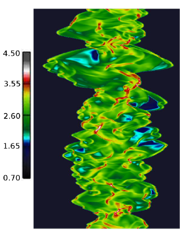
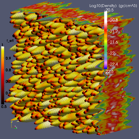
Figure 1: Different geometry of confining shocks. In 2D (periodic in y-direction, infinite in z-direction), the confining shocks resemble corrugated sheets (left panel). In 3D (periodic in y- and z-direction) they evoke the idea of cardboard egg wrappings (right panel). Both simulations have $M_{\mathrm{u}}=21.7$. Color coded is density (log10($\rho$); particles/cm³ in 2D; g/cm³ in 3D) and, right panel only, the driving efficiency $f_{\mathrm{eff}}$ at the shock surface.

2.4 Data analysis

The relevant quantity for the time evolution of CDL quantities is the average x-extension of the CDL, $\ell_{\mathrm{cdl}}\equiv V/(\mathrm{Y}\mathrm{Z})$ with $V$ the volume of the CDL (see Sect. 3 or the 2D case in FW06). The average CDL extension does, however, not need to be a strictly monotonically increasing function of time, as the CDL compression fluctuates slightly with time.

A proxy to $\ell_{\mathrm{cdl}}$ that does not show such fluctuations can be defined through the monotonically increasing CDL mass. Expressing $\ell_{\mathrm{cdl}}$ in terms of the CDL mass $m_{\mathrm{cdl}}$ and mean density $\rho_{\mathrm{m}}$ as $\ell_{\mathrm{cdl}}=m_{\mathrm{cdl}}/(\rho_{\mathrm{m}}\mathrm{Y}^{2})$, where we used $\mathrm{Y}=\mathrm{Z}$, we can replace $\rho_{\mathrm{m}}$ by $\rho_{\mathrm{u}}$ and normalize with $\mathrm{Y}$ to obtain a monotonically increasing, dimensionless quantity, $\ell\equiv m_{\mathrm{cdl}}/(\rho_{\mathrm{u}}\mathrm{Y}^{3})$.

All simulations were advanced till at least $\ell=12$, some much further. Except for the lowest Mach number simulations, $\ell\approx 12$ corresponds to within 10% to a spatial extent of $\mathrm{Y}/2$, i.e., the x-extension of the CDL is about half the domain size in yz-direction. Data analysis is done off-line, on previously dumped data sets. Temporal averages, unless otherwise stated, are taken over $\ell\in[11,12]$. This interval comprises at least three data sets.

Part of the data analysis was done with VisIt, combined with python scripting. We developed a reader for VisIt that can cope with our block structure adaptive mesh refinement data, stored in hdf5 format. VisIt proved particularly useful for the slice wise analysis of the data (see Sect. 3.2.3) and for the numerical determination of the driving efficiency. The latter involves local decomposition of the upstream flow into components perpendicular and parallel to the confining shocks and integration over these shocks (see Appendix A). We use VisIt to create an iso-surface representative of the confining shock, defined by a density threshold slightly greater than $\rho_{\mathrm{u}}$, and then exploit VisIts capabilities of providing surface normals to iso-surfaces. An example of the reconstructed shock surface, colored in driving efficiency $f_{\mathrm{eff}}$ (see Eq. 9), is shown in Fig. 1, right panel.

3 Results

The section is structured along two main perspectives: the view on the CDL as an entity and the view on its interior structure. In Sect. 3.1, we concentrate on approximate scaling relations for some CDL mean quantities in 1D to 3D. In Sect. 3.2 we focus on the anisotropy and inhomogeneity of the CDL interior. 2D slices are used to analyze how mean quantities change with distance from the CDL center. Sect. 3.3 is dedicated to density PDFs, Sect. 3.4 to structure functions. The physical results are complemented by considerations on numerical resolution in Sect. 3.5.

3.1 CDL Mean quantities: approximate scaling relations

Within the frame of Euler equations, i.e., in the absence of viscous dissipation, and making some further assumptions as detailed below, approximate self-similar scaling relations for CDL mean quantities can be derived and expressed in terms of upstream flow parameters. The relations are qualitatively different in 1D as compared to 2D and 3D (see FW06). In particular, in 1D the mean density increases with the upstream Mach number squared. In 2D / 3D the CDL mean density is expected to be limited, the root mean square Mach number should increase linearly with the upstream Mach number.

3.1.1 Analytical scaling relations for CDL mean quantities

Looking first at the 1D case and denoting the density and velocity of the CDL by $\rho_{\mathrm{1d}}$ and $v_{\mathrm{1d}}$, those of the left and right upwind flows by $\rho_{\mathrm{i}}$ and $v_{\mathrm{i}}$ ($i=l,r$), and the isothermal sound speed by $a$, it can be shown that (e.g., Courant & Friedrichs, 1976) in the rest frame of the CDL

$$\rho_{\mathrm{1d}}/\rho_{\mathrm{i}} = M_{\mathrm{i}}^{\mathrm{2}}+1\approx M_{\mathrm{i}}^{2},$$ (1)

$$v_{\mathrm{1d}} = 0.$$ (2)

The approximation holds for large Mach-numbers. A relation between characteristic length and time scales of the solution, the self-similarity variable $\kappa_{\mathrm{1d}}$, can be obtained as the ratio between the spatial extension $\ell_{\mathrm{1d}}$ of the CDL and the time $\tau$ needed to accumulate the corresponding column density ${N}_{\mathrm{1d}}$:

$$N_{\mathrm{1d}}=\rho_{\mathrm{1d}}\ell_{\mathrm{1d}},$$ (3)

$$N_{\mathrm{1d}}=\tau\left(\rho_{l}v_{l}+\rho_{r}v_{r}\right),$$ (4)

and using $\rho_{\mathrm{l}}/\rho_{\mathrm{r}}=M^{2}_{\mathrm{r}}/M^{2}_{\mathrm{l}}$

$$\kappa_{\mathrm{1d}}\equiv\frac{\ell_{\mathrm{1d}}}{\tau}=a\frac{M_{l}+M_{r}}{M_{l}\cdot M_{r}}.$$ (5)

For strong shocks and symmetric settings ($\mathrm{l}=\mathrm{r}$) the above relations reduce to $\rho_{\mathrm{1d}}/\rho_{\mathrm{u}}=M_{\mathrm{u}}^{2}$ and $\kappa_{\mathrm{1d}}=2a/M_{\mathrm{u}}$.

For the 2D case, FW06 derived scaling relations for five CDL mean quantities: mean density $\rho_{\mathrm{m}}$; root mean square Mach number $M_{\mathrm{rms}}$; driving energy $\dot{\cal E}_{\mathrm{drv}}$, i.e., the kinetic energy density entering the CDL per time and unit length in the y-direction; $\dot{\cal E}_{\mathrm{diss}}$, the energy density dissipated per time within an average column of length $\ell_{\mathrm{cdl}}$; the change per time of the average kinetic energy energy density contained within such an average column, $\dot{\cal E}_{\mathrm{kin}}$.

Extension to 3D is straightforward. The only derivation we repeat here (see Appendix A) is that of the driving energy $\dot{\cal E}_{\mathrm{drv}}$, which involves an integral over the confining shocks. Part of the total (left plus right flow) upwind kinetic energy flux density, ${\cal F}_{\mathrm{e_{\mathrm{kin}},u}}=\rho_{\mathrm{u}}v_{\mathrm{u}}^{3}$, is thermalized at these shocks. The remaining part, $\dot{\cal E}_{\mathrm{drv}}$, drives the turbulence in the CDL. In analogy with the 2D case, we write $\dot{\cal E}_{\mathrm{drv}}=f_{\mathrm{eff}}{\cal F}_{\mathrm{e_{\mathrm{kin}},u}}$, where the driving efficiency $f_{\mathrm{eff}}$ is a function of the upwind Mach-number alone. The formal dependencies, involving upstream quantities $\rho_{\mathrm{u}}$ and $M_{\mathrm{u}}$, as well as parameters $\beta_{\mathrm{i}}$ and $\eta_{\mathrm{i}}$ (to be determined), are as in the 2D case:

$$\rho_{\mathrm{m}} = \eta_{\mathrm{1}}\rho_{\mathrm{u}}M_{\mathrm{u}}^{\beta_{\mathrm{1}}}=\eta_{\mathrm{1}}\rho_{\mathrm{u}},$$ (6)

$$M_{\mathrm{rms}} = \eta_{\mathrm{2}}M_{\mathrm{u}}^{\beta_{\mathrm{2}}}=\eta_{\mathrm{1}}^{-1/2}M_{\mathrm{u}},$$ (7)

$$\kappa_{\mathrm{3d}} = \ell_{\mathrm{cdl}}/\tau=2\eta_{\mathrm{1}}^{-1}aM_{\mathrm{u}},$$ (8)

$$f_{\mathrm{eff}} = (1-\eta_{\mathrm{3}}M_{\mathrm{u}}^{\beta_{\mathrm{3}}}),$$ (9)

$$\dot{\cal E}_{\mathrm{drv}} = \rho_{\mathrm{u}}a^{3}M_{\mathrm{u}}^{3}(1-\eta_{\mathrm{3}}M_{\mathrm{u}}^{\beta_{\mathrm{3}}}),$$ (10)

$$\dot{\cal E}_{\mathrm{kin}} = \rho_{\mathrm{u}}a^{3}M_{\mathrm{u}}^{3}\;\eta_{\mathrm{2}}^{2},$$ (11)

$$\dot{\cal E}_{\mathrm{diss}} = \rho_{\mathrm{u}}a^{3}M_{\mathrm{u}}^{3}(1-\eta_{\mathrm{3}}M_{\mathrm{u}}^{\beta_{\mathrm{3}}}-\eta_{\mathrm{2}}^{2}).$$ (12)

Here, $\beta_{\mathrm{1}}=0$ and $\beta_{\mathrm{2}}=1$ from analytical considerations, whereas $\beta_{\mathrm{3}}$ as well as $\eta_{\mathrm{i}}$, $i=1,2,3$, can be determined only from numerical simulations and turn out to be different in 2D and 3D. The 3D numerical results, to be presented in Sect. 3.1.2, confirm $\beta_{\mathrm{1}}=0$ and $\beta_{\mathrm{2}}=1$, and yield $\beta_{\mathrm{3}}\approx-1.17$, $\eta_{\mathrm{1}}\approx 25$, $\eta_{\mathrm{2}}\approx 0.2$, and $\eta_{\mathrm{3}}\approx 5$ as best fit values.

The above relations imply that the mean density of the CDL does not depend on the upstream Mach number $M_{\mathrm{u}}$, in strong contrast to the 1D case where $\rho_{\mathrm{m}}\propto M_{\mathrm{u}}^{2}$. The CDL root mean square Mach number should increase linearly with $M_{\mathrm{u}}$. Also: the larger $M_{\mathrm{u}}$, the larger $f_{\mathrm{eff}}$, i.e., the more energy passes the confining shocks of the CDL unthermalized

We stress the four basic assumptions made in deriving the above relations: a) a simple Mach-number dependency of $\rho_{\mathrm{m}}$, $v_{\mathrm{rms}}$, and $f_{\mathrm{eff}}$; b) CDL density and velocity are uncorrelated; c) we have high Mach-numbers in the sense that $\eta_{\mathrm{2}}^{2}M_{\mathrm{u}}^{2\beta_{\mathrm{2}}}>>1$ or $M_{\mathrm{rms}}^{2}>>1$; d) $v_{\mathrm{diss}}\propto v_{\mathrm{rms}}$. For a discussion of the validity of these assumptions we refer to FW06.

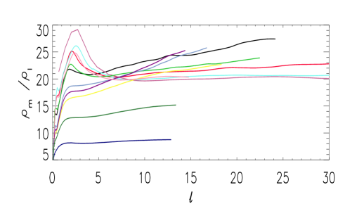
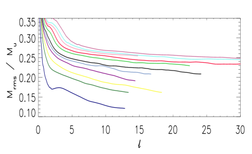
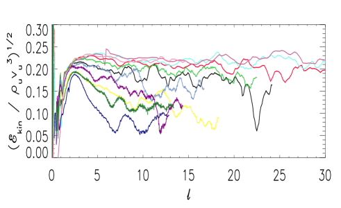
Figure 2: Mean density $\rho_{\mathrm{m}}$ (top panel), root mean square Mach number $M_{\mathrm{rms}}$ (middle panel), and $(\dot{\cal E}_{\mathrm{kin}}/(\rho_{\mathrm{u}}a^{3}M_{\mathrm{u}}^{3}))^{1/2}$ (bottom panel) as function of the monotonically increasing CDL size $\ell$ for simulations R*_2. Individual curves denote $M_{\mathrm{u}}=2$ (dark blue), 4 (dark green), 5 (yellow), 7 (purple), 8 (light blue), 11 (black), 16 (green), 22 (red), 27 (pink), 33 (cyan), and 43 (magenta).

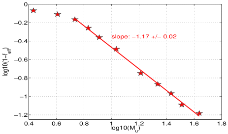
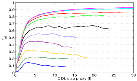
Figure 3: Driving efficiency of 3D slabs, same simulations and color coding as in Fig. 2. Top panel: Comparison of numerical results with expected scaling relation $\beta_{\mathrm{3}}\mathrm{log}_{\mathrm{10}}(M_{\mathrm{u}})\propto\mathrm{log}_{\mathrm{10}}(1-f_{\mathrm{eff}})$. Each star denotes the maximum driving efficiency of one simulation. Bottom panel: Evolution of $f_{\mathrm{eff}}$ as function of CDL size.

3.1.2 3D scaling relations: numerical results

The analytical relations in Eq. 6 to 12 basically state that CDL mean quantities can be expressed in terms of upstream quantities and that the corresponding relations do not change with time / CDL size. Comparing the analytical predictions with our numerical results thus means checking for two things: do the relations hold across simulations, i.e., across widely varying upstream Mach numbers, and do the relations hold independent of time / CDL size.

We first focus on the comparison of analytical and numerical results with regard to the first question, the validity of the analytical relations across different upstream Mach numbers. In doing so, we tacitly assume that $\beta{\mathrm{i}}$ and $\eta_{\mathrm{i}}$ do not change with time / CDL size.

Looking first at $\rho_{\mathrm{m}}$, Fig. 2, top panel, and ignoring for the moment the obvious drift with increasing CDL thickness, and concentrating instead on CDL thicknesses $6\leq\ell\leq 12$, the density compression ratios can be seen to lie mostly in a range of $20\leq\eta_{\mathrm{1}}\leq 25$. This narrow range is remarkable given the range of upstream Mach numbers ($2.7\leq M_{\mathrm{u}}\leq 43.4$) and the associated 1D compression ratios ( $7<\rho_{\mathrm{1d}}/\rho_{\mathrm{u}}<1900$). The only clear exceptions here are simulation R2_2 and R4_2, whose upstream Mach numbers allow at most for 1D compression factors of about 7 and 16, respectively, roughly the values attained also in the 3D case (dark blue and dark green curves in Fig. 2). The analytically predicted value of $\beta_{\mathrm{1}}=0$ is confirmed by the numerical results in that the scatter among the different curves in Fig. 2, top panel, cannot be improved by any other choice for $\beta_{\mathrm{1}}$.

For the root mean square Mach number (Fig. 2, middle panel), we find $\eta_{\mathrm{2}}=M_{\mathrm{rms}}/M_{\mathrm{u}}=0.25$ to within about 10% for all simulations except those with very low upstream Mach number ($M_{\mathrm{u}}\leq 7$). As in the case of density, changing the predicted dependence of $M_{\mathrm{rms}}$ on $M_{\mathrm{u}}$ does not reduce the scatter of the curves, unless low Mach number simulations are included, in which case $\beta_{\mathrm{2}}=1.1$ or even 1.2 gives a smaller spread among curves than the predicted value of $\beta_{\mathrm{2}}=1$. Using Eq. 7, the above range for $\eta_{\mathrm{2}}$ implies for $\eta_{\mathrm{1}}=\eta_{\mathrm{2}}^{-2}$ a value in the range from 13 to 20, somewhat smaller but roughly consistent with the numerically obtained density compression ratios discussed above. Better consistency is achieved if $\eta_{\mathrm{2}}$ is determined using Eq. 11 instead of Eq. 7. From Fig. 2, bottom panel, and neglecting again low Mach number simulations, we find $\eta_{\mathrm{2}}\approx 0.2$, which corresponds to $\eta_{\mathrm{1}}\approx 25$. We ascribe the ambiguity in the numerical value of $\eta_{\mathrm{2}}$ to slight violations of the underlying assumptions in deriving Eq. 6 to 12, in the case of low Mach number simulations especially the assumption that $M_{\mathrm{rms}}>>1$.

Numerical results regarding the remaining scaling relations, those involving the driving efficiency $f_{\mathrm{eff}}$ and associated parameters $\eta_{\mathrm{3}}$ and $\beta_{\mathrm{3}}$, are shown in Fig. 3. The top panel relates the maximum driving efficiency achieved in each simulation with its upstream Mach number. For $M_{\mathrm{u}}\geq 5$, an excellent linear relation ship between log($M_{\mathrm{u}}$) and log($1-f_{\mathrm{eff}}$) is found with slope $\beta_{\mathrm{3}}=-1.17\pm 0.02$ and $\eta_{\mathrm{3}}=5$.

Changing perspective and looking at the evolution with CDL thickness (or time) in Fig. 2, all simulations show a persistent and clear decrease of the root mean square Mach number with time and an associated increase of the density compression ratio, in clear disagreement with the expected scaling relations. In units $M_{\mathrm{rms}}/M_{\mathrm{u}}$, the decrease is about the same for all simulations, around 0.02 to 0.03 (between about 10% and 20%) for a doubling of the CDL thickness $\ell$ from 6 to 12. Relative changes are more pronounced for simulations with smaller $M_{\mathrm{u}}$.

The same effect was observed in the 2D case and there attributed to the increasing role of numerical dissipation with increasing CDL size (FW06). We favor the same explanation given there also for the 3D case. The volume (or mass) fraction of the CDL that is subsonic remains about constant with time (Fig. 4). In absolute terms, the subsonic parts of the CDL grow as the CDL grows. Energy loss in these parts, dominated by numerical dissipation / viscous dissipation in terms of the MILES approach, grows in proportion - while $\dot{\cal E}_{\mathrm{drv}}\approx\mathrm{const.}$. The effect leads to an overall decay of CDL turbulence. It is more severe for smaller $M_{\mathrm{u}}$, as a larger fraction of the CDL is subsonic (Fig. 4), thus in violation of the assumptions made in deriving the analytical scaling relations in Sect. 3.1.1.

Similar drifts with time exist for the driving efficiency, Eq. 9 and Fig. 3 (bottom panel). However, considering again the period $6\leq\ell\leq 12$, the drifts with time of $f_{\mathrm{eff}}$ can be to either larger or smaller values. Apparently, the larger $M_{\mathrm{u}}$, the larger the CDL has to grow before the driving efficiency reaches its peak value.

In summary, we conclude from the above findings that the numerical results essentially confirm the validity of the self-similar analytical relations Eqs. 6 to 12 across different upstream Mach numbers, although the numerical results display a systematic drift with increasing CDL size, which we attribute to the effect of numerical dissipation / viscous dissipation.

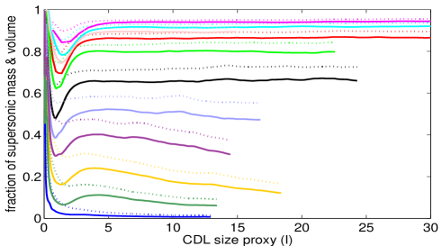
Figure 4: Supersonic mass fraction (solid) and volume fraction (dotted), color coding as in Fig. 2.

3.2 Inhomogeneity and anisotropy of CDL

The driving of the turbulence within the CDL is highly anisotropic and inhomogeneous: energy is injected only at the two confining shocks of the CDL and only in the form of flows directed parallel or anti-parallel to the x-axis. The amount of kinetic energy entering the CDL, as well as its decomposition into compressible and solenoidal components, depends on the orientation of the confining shock with respect to the upstream flow and thus changes with position along the confining shock. It is thus to be expected that the turbulence within the CDL is neither homogeneous, nor isotropic. Viewing angle effects in observational data are a logical consequence.

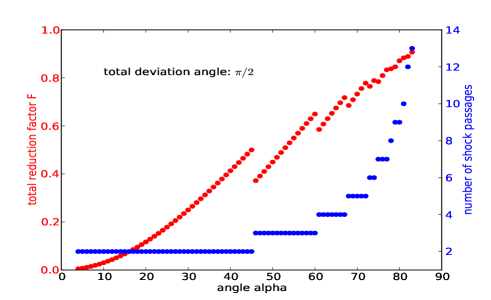
Figure 5: Deviating a highly supersonic, isothermal flow by (at least) $\beta_{\mathrm{tot}}=\pi/2$ through $n$ (right y-axis) subsequent shock passages at angle $\alpha$ (x-axis; in degrees; angle between flow direction and surface normal of shock) results in a total reduction of the Mach number by a factor $F_{\mathrm{tot}}$ (left y-axis).

3.2.1 Mach number anisotropy

From Table 1 it can be taken that the CDL root mean square Mach number is highly anisotropic. Root mean square Mach numbers in direction transverse to the upstream flow (yz-plane, $M_{\mathrm{rms,\perp}}$) are subsonic in all our experiments, with concrete Mach numbers ranging from about 0.2 to 0.8. In the direction parallel to the upstream flow, supersonic root-mean-square Mach numbers $M_{\mathrm{rms,\parallel}}$ are found from R7_2 onwards. The ratio $M_{\mathrm{rms,\parallel}}/M_{\mathrm{rms,\perp}}$ ranges from around 2 to over 11.

Indeed, analytical considerations show the difficulty associated with substantially deviating isothermal head-on colliding flows, a necessary condition to reach isotropic conditions, while retaining supersonic flow conditions. To illustrate the point, look at a uniform flow hitting an oblique shock. Let $\alpha$ denote the angle between the flow direction and the surface normal of the shock. Decomposing the upstream and downstream flow velocities, $\mathbf{v}_{\mathrm{u}}$ and $\mathbf{v}_{\mathrm{d}}$, into components parallel and perpendicular to the shock, assuming $M_{\mathrm{u}}>>1$, and applying isothermal shock jump conditions $v_{\mathrm{d}\perp}=v_{\mathrm{u}\perp}M_{\mathrm{u}\perp}^{-2}$, one can write

$$\mathbf{v}_{\mathrm{u}} = \mathbf{v}_{\mathrm{u\parallel}}+\mathbf{v}_{\mathrm{u\perp}}=v_{\mathrm{u}}\mathrm{sin}\alpha\;\mathbf{e}_{\mathrm{\parallel}}+v_{\mathrm{u}}\mathrm{cos}\alpha\;\mathbf{e}_{\mathrm{\perp}}$$ (13)

$$\mathbf{v}_{\mathrm{d}} = \mathbf{v}_{\mathrm{d\parallel}}+\mathbf{v}_{\mathrm{d\perp}}=v_{\mathrm{u}}\mathrm{sin}\alpha\;\mathbf{e}_{\mathrm{\parallel}}+v_{\mathrm{u}}\mathrm{cos}\alpha\;M_{\mathrm{u}}^{-2}\mathrm{cos}^{-2}\alpha\;\mathbf{e}_{\mathrm{\perp}}.$$ (14)

These relations can be recast in the form of the Mach number reduction factor $F\equiv v_{\mathrm{d}}/v_{\mathrm{u}}$ and the deviation angle $\beta$ between the upstream and the downstream flow direction,

$$F \equiv \frac{v_{\mathrm{d}}}{v_{\mathrm{u}}}=(1-\mathrm{cos}^{2}\alpha-\mathrm{cos}^{-2}\alpha\;M_{\mathrm{u}}^{-4})^{1/2}\approx\mathrm{sin}\alpha$$ (15)

$$\beta = \mathrm{arccos}\left(\frac{\mathbf{v}_{\mathrm{u}}\cdot\mathbf{v}_{\mathrm{d}}}{v_{\mathrm{u}}v_{\mathrm{d}}}\right)\approx\mathrm{arccos}(F)=\frac{\pi}{2}-\alpha,$$ (16)

where the approximations hold for large $M_{\mathrm{u}}$ and angles $\alpha$ not too close to either $0$ or $\pi/2$. From Eqs. 15 and 16 it is apparent that large deviation angles $\beta$ come at the price of substantial reduction factors $F$, at least for single shock passages. Multiple ’grazing’ shock passages (large $\alpha$) allow, in principle, for large total deviation angles $\beta_{\mathrm{tot}}$ while retaining an overall reduction factor $F_{\mathrm{tot}}$ close to one. For $n$ subsequent shock passages at the same angle $\alpha$ one has $\beta_{\mathrm{tot}}=n\;(\pi/2-\alpha)$ and $F_{\mathrm{tot}}=(\mathrm{sin}\alpha)^{n}$. The situation is illustrated in Fig. 5 for $\beta_{\mathrm{tot}}\geq\pi/2$. For example, two subsequent shock passages at $\alpha=\pi/4$ allow for a total deviation of $\pi/2$ while retaining about half of the initial upstream Mach number ($F_{\mathrm{tot}}\approx 0.5$), while seven passages at an angle of close to $80^{\circ}$ are needed to retain 80% of $M_{\mathrm{u}}$. From Fig. 5 it can also be taken that already one shock passage at an angle $\alpha<30^{\circ}$ reduces $M_{\mathrm{u}}$ by at least 75%.

It is this later situation, even a few shock passages at small angles $\alpha$, which we believe to be responsible for the low transverse Mach numbers in our 3D slabs, despite the generally rather ’grazing’ angles at the confining shocks.

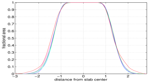
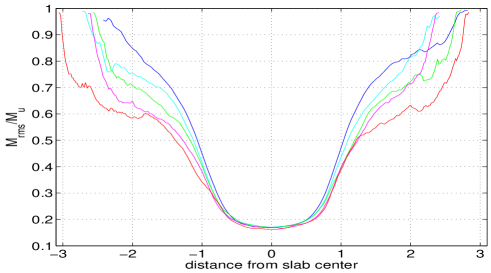
Figure 6: 2D slice (yz-plane) averages as function of (scaled) x-coordinate for R22_2 for different times ($\ell=12,17,23,29,$ and $34$, for the blue, cyan, green, magenta, and red curves, respectively). Top panel: Fractional 2D CDL area $F(x)$. Bottom panel: Root mean square Mach number in units of $M_{\mathrm{u}}$. For details see text, Sect. 3.2.3.

3.2.2 Density variance - Mach number relation

This anisotropy of $M_{\mathrm{rms}}$ carries over to the density variance - Mach number relation,

$$\frac{\sigma(\rho)}{\rho_{\mathrm{m}}M_{\mathrm{rms}}}=b.$$ (17)

From 3D periodic box simulations of driven, isothermal, supersonic, hydrodynamical turbulence a value of $b\in[1/3,1]$ is found, depending on the nature of the forcing, purely compressible ($b=1$) or purely solenoidal ($b=1/3$) (Padoan et al., 1997; Passot & Vázquez-Semadeni, 1998; Federrath et al., 2010).

Using Eq. 17 for our CDL with $M_{\mathrm{rms}}$ the total root-mean-square Mach number, we find $b\in[0,1/3]$ (see Table 1), a range hardly overlapping with 3D periodic box results. Higher $b$-values are obtained for the CDL if only the transverse component $M_{\mathrm{rms,\perp}}$ is considered: around 0.6 to 0.7 for small $M_{\mathrm{u}}$ and up to 0.85 for large $M_{\mathrm{u}}$. In the context of turbulence in flow collision zones, the density variance - Mach number relation thus seems rather indicative of the viewing angle (line-of-sight along $M_{\mathrm{rms,\parallel}}$ or $M_{\mathrm{rms,\perp}}$) than of the driving of the turbulence.

3.2.3 Role of distance to confining shocks: 2D slices

CDL quantities are not only anisotropic, but they also differ between regions close to the confining shocks, the only place where energy is injected into the CDL, and areas close to the central plane of the CDL. What ’close to the confining shocks’ really means may be debated. One interpretation could be to study flow properties as a function of distance from the confining shock. This we will not attempt here, as our spatial resolution is likely too coarse anyway to capture the details of such ’boundary layer flows’.

Instead, we study how averages over 2D slices (yz-plane) of the CDL vary with the position of the slice from the CDL center. Technically speaking, we take 2D slices (yz-plane) at different positions along the x-axis, identify those cells within a given slice that belong to the CDL (and not the upstream flow) by checking for $M_{\mathrm{rms}}<M_{\mathrm{u}}$, and compute average quantities for each such 2D CDL area $A(x)$. Introducing the fractional 2D CDL area $F(x)=A(x)/(YZ)$, with $YZ$ the yz-cross-section of the computational domain, slices close to the CDL center are characterized by $F(x)=1$, whereas slices close to outermost tips of the confining shocks have $F(x)\approx 0$. To plot the resulting 2D averages, we use scaled x-units, which we define by mapping the core part of the CDL with $F(x)>0.9$ onto the interval [-1,1] in scaled x-units. We expect this mapping to make sense because of (approximate) self-similarity. This is confirmed by Fig. 6, top panel: the curves for the fractional 2D CDL area $F(x)$ as a function of scaled x-units (simulation R22_2) fall essentially on top of each other, although the CDL size increases from $\ell\approx 12$ to $\ell\approx 34$. Similar figures are obtained for other simulations.

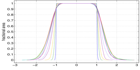
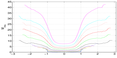
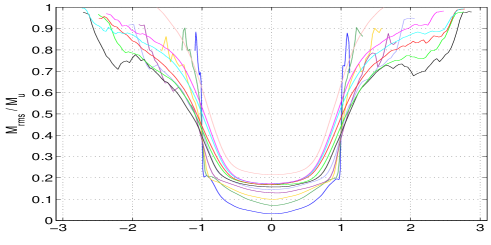
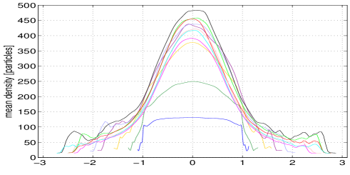
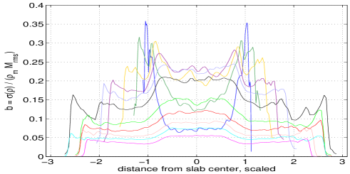
Figure 7: 2D slices, average quantities for different runs (color coding as in Fig. 2) at CDL size $\ell\approx 12$. From top to bottom: fractional CDL area $F(x)$, root mean square Mach number $M_{\mathrm{rms}}$, scaled root mean square Mach number $M_{\mathrm{rms}}/M_{\mathrm{u}}$, mean density $\rho_{\mathrm{m}}$, and $b=\sigma(\rho)/(\rho_{\mathrm{m}}M_{\mathrm{rms}})$.

Denoting parts where $F(x)<1$ as ’CDL boundary layer’ and parts with $F(x)=1$ as ’CDL core region’, Fig. 6, top panel, further shows that the relative widths of the ’CDL boundary layer’ as compared to the ’CDL core region’ remain essentially constant throughout the simulation. The boundary layer does not increase with respect to the core region or vice versa, the spatial extension of each part obeys approximate self-similarity again. Within the ’CDL boundary layer’, $M_{\mathrm{rms}}$ generally decreases with time for any given fixed relative x-position (Fig. 6, bottom panel). A possible explanation for the decrease could be that as the CDL gets wider, individual wiggles of the confining shocks extend farther and comprise larger volumes (’get fatter’), the surface to volume ratio decreases. In a 2D cut half way between $F(x)=0.9$ and $F(x)\approx 0$, the CDL patches get larger for larger CDL thickness $\ell$. The distance from the patch center to its boundary - the confining shock where energy is injected - gets larger. The patch area (where turbulence must be driven) divided by the patch circumference (where energy is injected) gets larger.

Passing from one simulation at different times to comparison of different simulations for the same CDL size, as shown in Fig. 7 for different quantities, reveals again the prominent role of the upstream Mach number. Larger upstream Mach numbers result in larger ’CDL boundary layers’, relative to the ’CDL core region’ (Fig. 7, first panel). The root mean square Mach number in the ’CDL core region’ is slightly lower than the CDL mean (around 15% to 20% of $M_{\mathrm{u}}$, second and third panel of Fig. 7). The density distribution is more peaked around the CDL center than the $M_{\mathrm{rms}}$ distribution (Fig. 7, fourth panel). Consistent with CDL mean values of Sect. 3.1, the largest densities are reached for intermediate upstream Mach numbers, not for the highest. A tentative interpretation here is that low upstream Mach numbers, on the one hand, cannot generate the necessary compression, whereas high upstream Mach numbers generate too Much turbulence, leading again to somewhat lower mean densities. Numerical limitations (resolution) to maximum compression ratios may also play a role (see Sect. 3.5). Finally, the density variance-Mach number relation shows less and less dependence on the slice position with increasing $M_{\mathrm{u}}$ (Fig. 7, fifth panel)

In summary, the analysis in terms of 2D slices illustrates the inhomogeneity of the CDL turbulence, the CDL core region is less turbulent than the CDL boundary layer. The relative weight of core and boundary layer is independent of the CDL extension.

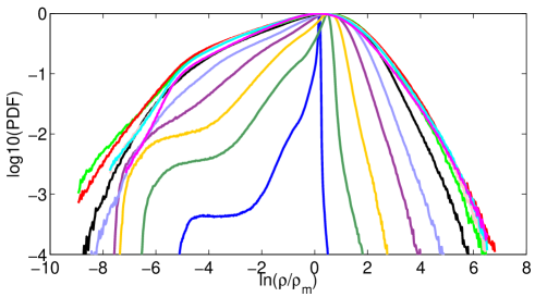
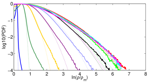
Figure 8: Top panel: Volume-weighted PDFs of $s=ln(\rho/\rho_{m})$ for the different runs, color coding as in Fig. 2. Each curve is an average over three data sets between $\ell\approx 11$ and $\ell\approx 12$. Bottom panel: Centrally (at peak value of PDF) mirrored PDF with Gaussian fitting (dotted line).

3.3 Density probability distribution function

The probability distribution function (PDF) of turbulent density fluctuations is of key interest in connection with star formation and as such extensively covered in the literature (e.g., Padoan & Nordlund, 2002; Krumholz & McKee, 2005; Hennebelle & Chabrier, 2011). A number of studies suggest that the density PDF of isothermal, isotropic, and homogeneous supersonic turbulence is log-normal, i.e., $s=\mathrm{ln}(\rho/\rho_{m})$ follows a Gaussian distribution (e.g., Vazquez-Semadeni, 1994; Passot & Vázquez-Semadeni, 1998). The PDF may deviate from a log-normal distribution if additional physics is included, e.g., self-gravity, or if subsonic root mean square Mach numbers result from solenoidal forcing (Federrath et al., 2009; Kitsionas et al., 2009).

The PDFs of $\mathrm{ln}(\rho/\rho_{m})$ we find for our different runs also clearly deviate from a log-normal distribution (Fig. 8, top panel). Each PDF is the average over three snapshots of the CDL with seizes $\ell\in[11,12]$.

To the right of their maxima, the PDFs can be approximately captured by a log-normal distribution, but typically have a fat tail (Fig. 8, bottom panel). The fit (dotted line) was obtained by first mirroring the right half of the PDF at its peak, then determining the FWHM $w$ of the resulting distribution, from which $\sigma$ can be obtain using $w=2(2ln(2))^{1/2}\sigma$ and assuming that the distribution is normal.

To the left of their maxima, the PDFs show a more intricate structure. For runs with $M_{\mathrm{rms}}<1$, the peak value decreases sharply before a plateau region is formed. This plateau region is likely associated with grid cells close to or even within the confining shocks of the CDL, which on numerical grounds are about 3 cells wide. Except for this plateau region, the shape of the PDFs at these low Mach numbers resembles density PDFs found by Kitsionas et al. (2009) for 3D periodic box simulations with purely solenoidal forcing at subsonic root mean square Mach numbers. As we go to higher Mach numbers, the decline of the PDF to the left of its peak value becomes shallower, reaching about a constant slope for runs with $M_{\mathrm{u}}>11$. The plateau region of the low Mach number runs turns into a steep slope for the high Mach number runs.

In summary, despite having purely isothermal conditions and no additional physics, like for example self-gravity, the density PDFs of our CDL always remain far from a log-normal distribution, even if the turbulence is highly supersonic (large $M_{\mathrm{rms}}$).

3.4 Structure functions

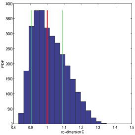
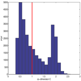
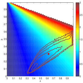
Figure 9: A 5% random perturbation of $Z_{p}$ (30 000 realizations, at the example of $Z_{p}$ from Boldyrev (2002), $p=1$ to $p=5$) causes smearing of co-dimensions $C$ derived from Eq. 20 (left panel). A double peak distribution results if $C$ is computed from Eq. 21 (middle panel). The analytical value $C=1$ is shown as a red line, green lines in the left panel indicate where the 2/3 largest values in the histogram are located. In the right panel, the 2D histogram (log10 contours, spacing 0.5, spanning three orders of magnitude) of co-dimensions from perturbed $Z_{p}$ (500 000 realizations) is over-plotted on the co-dimension $C=\Delta/(1-\beta)$ (color coded) in the $\Delta$-$\beta$ plane (Eq. 21). Two sharp peaks can be distinguished, at $\Delta\approx 0.4$ and $\beta\approx 0.1$ ($C\approx 0.44$), as well as at $\Delta\approx 1.0$ and $\beta\approx 0.5$ ($C\approx 1.9$). The red dot is the analytical value by Boldyrev (2002), $\Delta=2/3$, $\beta=1/3$, $C=1$.

Since the seminal work of Kolmogorov (1941) (K41), velocity structure functions have become an established tool for the characterization of isotropic, homogeneous, incompressible, and stationary turbulence. By contrast, the understanding of anisotropic, inhomogeneous, compressible, non-stationary, or bound turbulence is only in its infancy (Kurien & Sreenivasan, 2000; Biferale et al., 2008; Byrne et al., 2011; Hansen et al., 2011; Biferale et al., 2012; Grauer et al., 2012). Characterizing our CDL data in terms of structure functions thus is rather exploratory. We nevertheless consider presentation of associated results worthwhile, to make a few first steps in this direction, to compare our setup with results from 3D periodic box simulation, and to illustrate the potential role of line-of-sight effects, the latter also in view of published, observation based structure functions for molecular clouds whose physical interpretation continues to be debated (e.g., Padoan et al., 2003; Gustafsson et al., 2006; Hily-Blant et al., 2008).

3.4.1 Working with low resolution CDL data

Anticipating quantitative values given in Sect. 3.4.2, here we first want to carve out two implications of the low resolution of our CDL data: the compelling use of extended self-similarity and why we determine the co-dimension of the most dissipative structure by using the one parameter expression of Eq. 20 instead of the two parameter expression of Eq. 21. We also introduce some notation used later on.

The structure function of order $p$ is a scalar function of distance $r$, defined as

$$S_{p}(r)\equiv<|\mathbf{u}(\mathbf{x}+\mathbf{r})-\mathbf{u}(\mathbf{x})|^{p}>,$$ (18)

where $<\dots>$ denotes the average over all positions $\mathbf{x}$ within the sample and over all directed distances $\mathbf{r}$ from each position. Structure functions are termed longitudinal ($S_{p}^{\parallel}$) if only orientations $\mathbf{u}\parallel\mathbf{r}$ enter the average, and perpendicular ($S_{p}^{\perp}$) if only $\mathbf{u}\perp\mathbf{r}$ enters. In the inertial range, both can be well approximated by power laws with scaling exponents $\zeta_{p}$

$$S_{p}(r)\propto r^{\zeta_{p}}.$$ (19)

The numerical determination of $\zeta_{p}$ is difficult if the inertial range is small, as is the case for our data (see Sect. 3.4.2). The extended self-similarity (ESS) hypothesis (Benzi et al., 1993) can remedy the situation to some extent. It basically states that the self-similarity of the velocity field, if it exists, extends beyond the usual inertial range, into the dissipation range. This extended range can be explored by considering not absolute scaling exponents $\zeta_{p}$ but ratios $Z_{p}=\zeta_{p}/\zeta_{3}$.

ESS scaling exponents $Z_{p}$ can be related to the co-dimension $C=3-D$ of the most dissipative structures (dimension $D$),

$$Z_{p}=\frac{\zeta_{p}}{\zeta_{3}}=\frac{p}{9}+C\left(1-\left(1-\frac{2}{3C}\right)^{p/3}\right).$$ (20)

For 1D vortex filaments $C=2$ (She & Leveque, 1994), for sheet-like structures $C=1$ (Boldyrev, 2002). Intermediate values of $C$ are found in numerical simulations (Padoan et al., 2004). From multi-phase 3D periodic box simulations Kritsuk & Norman (2004) find $D=2.3$, which is, as pointed out by the authors, surprisingly close to observationally determined fractal dimensions of molecular clouds (about 2.3, e.g., Elmegreen & Falgarone, 1996; Roman-Duval et al., 2010). Roughly speaking, velocity structure functions link the dimension of the most dissipative turbulent structures to (observable) velocity differences.

Behind the one-parameter ($C$) view of Eq. 20 is the two-parameter ($\Delta$ and $\beta$) expression for $Z_{p}$ by Dubrulle (1994),

$$Z_{p}=(1-\Delta)\frac{p}{3}+\frac{\Delta}{1-\beta}\left(1-\beta^{p/3}\right),$$ (21)

with $C=\Delta/(1-\beta)$. For $\Delta=0$, the K41 law is recovered. For incompressible turbulence, She & Leveque (1994) postulated $\Delta=2/3$ and with $\beta=2/3$ got $C=2$. For supersonic turbulence, Boldyrev (2002) kept $\Delta=2/3$ but chose $\beta=1/3$, giving $C=1$. There is, however, no reason why $\Delta=2/3$ should also apply in the supersonic case, and why one may collapse in this way the two-parameter model of Eq. 21 into the one-parameter model of Eq. 20.

Using Eq. 21 to determine $C$ thus seems preferential. However, in an application like ours, another factor comes into play: Eq. 21 is much more sensitive to uncertainties in the $Z_{p}$ than Eq. 20. Fig. 9 illustrates the point. We start with theoretical values $Z_{p}$ from Boldyrev (2002) for $p=1$ to $p=5$. We randomly perturb each $Z_{p}$ by at most 5% (our accuracy requirement for $Z_{p}$, see Appendix B.2), thus obtaining 30 000 perturbed data sets. For each data set, we determine $C$ as best fit to either Eq. 20 or Eq. 21 (best fit = smallest root mean square error between analytical $Z_{p}$, $p=1..5$, and $Z_{p}$ of perturbed data set). If Eq. 20 is used, the 5% perturbation (uncertainty) of $Z_{p}$ results in a smearing of $C$, with $C$ mostly in a range 0.9 to 1.1 (Fig. 9, left panel). Using Eq. 21 results in a distribution with two peaks at $C\approx 0.44$ and $C\approx 1.9$ (Fig. 9, middle panel). A similar dichotomy was reported by Kritsuk et al. (2007b) and by Schmidt et al. (2009). Seen in the $\Delta$-$\beta$-plane (Fig. 9, right panel) the 5% uncertainty in $Z_{p}$ translates into a whole band of ($\Delta$, $\beta$) pairs and associated co-dimensions ($\Delta\approx 0.4$ and $\beta\approx 0.1$ for $C\approx 0.44$; $\Delta\approx 1.0$ and $\beta\approx 0.5$ for $C\approx 1.9$).

In view of these results, whose deeper discussion is beyond the scope of this paper, we decided to use the more robust one parameter expression Eq. 20 to compute the co-dimension $C$ from the ESS exponents $Z_{p}$.

3.4.2 Computing structure functions, ESS scaling exponents, and co-dimensions from CDL data

To compute $S_{p}(r)$ we use data at $\ell\approx 12$. Only points $\mathbf{x}$ within the CDL may contribute, the number of points contributing to $S_{p}(r)$ therefore decreases with $r$. When a directed distance $\mathbf{r}$ leaves the CDL it is forbidden to re-enter. The computation, detailed in Appendix B, is repeated in four different ways. Spherical averaging in Eq. 18 (’unified’ case); spherical averaging but retaining only pairs ($\mathbf{x}$, $r$) for which all distances $r$ lie still within the CDL (’full in’ case); along a direction (line-of-sight, LOS) either perpendicular or parallel to the upstream flow. We stress that no density variations or radiative transfer effects are taken into account.

Given the small inertial range of our structure functions, apparent in Fig. 10, top panel, we make use of the ESS hypothesis and compute linear fits to $Z_{p}$, i.e., to $\mathrm{log10}(S_{p})$ versus $\mathrm{log10}(S_{3})$. For the ’full in’ case, the quality of the fits is illustrated in Fig. 10, bottom panel, for longitudinal structure functions and $p=2$. In Appendix B, the quality of the fits is illustrated for all cases considered (’full in’, ’unified’, different LOSs) for $Z_{5}$ (Fig. 14) and computational details are given. From $Z_{p}$, $p=1$ to $5$, a best estimate for the co-dimension $C$ is derived for each run (using Eq. 20). Our demand that the uncertainty of the linear fit to $Z_{p}$ is smaller than 5% translates roughly into an uncertainty of $\pm 0.1$ for $C$ (see Sect. 3.4.1 and Fig. 9).

3.4.3 CDL structure functions: case ’full in’

The ’full in’ case is the most likely to bare similarities, if any, with 3D periodic box simulations. This because our demand that all 20 rays lie inside the CDL (see Sect. 3.4.2) rather disfavors contributions from the vicinity of the confining shocks with their (narrow) wiggles, where turbulence is most inhomogeneous and anisotropic (see Sect. 3.2.3).

Looking at the third order structure functions in Fig. 10, top panel, five observations may be made. First, our numerical resolution (256 cells in y-z-direction) hardly allows for the formation of a proper inertial range. The approximately linear dependence on $r$ covers less than one order of magnitude in $r$. Scaling exponents $\zeta_{p}$ (see Eq. 19) thus cannot be determined directly with sufficient quality. Second, this rapid leveling off seems not related to changing statistics with distance $r$. It takes place at distances $r$ where the sample size has not yet decreased substantially (see Fig. 13, top panel). Third, larger values of $M_{\mathrm{u}}$ result in shallower slopes of $\mathrm{log10}(S_{3})$ versus $\mathrm{log10}(r)$ that level off earlier. Fourth, the scatter of third order structure functions due to changing $M_{\mathrm{u}}$ is larger for $S_{3}^{\perp}$ than for $S_{3}^{\parallel}$, even at small radii. $S_{3}^{\perp}$ typically also levels off earlier than $S_{3}^{\parallel}$. Fifth, slopes $\zeta_{3}^{\parallel}=1.26$ and $\zeta_{3}^{\perp}=1.29$ from 3D periodic box simulations at $M_{\mathrm{rms}}=6$ (Kritsuk et al., 2007a), black lines in Fig. 10, appear to form an upper limit to the slab turbulence studied here, which covers a range of $0.33<M_{\mathrm{rms}}<11.5$ (see Table 1).

ESS scaling exponents are given in Table 2. Noteworthy are the following points. Longitudinal structure functions are consistent with co-dimension $C\approx 1$ or $D\approx 2$, i.e., indicating shocks as the most dissipative structures. They may show a tendency toward larger co-dimension $C$ for larger $M_{\mathrm{u}}$. The tendency stems to a good part from $Z_{5}$, all other $Z_{p}$ show no clear dependence on $M_{\mathrm{u}}$. The fits to $Z_{5}$ look reasonable (see Fig. 14, top left), but firm conclusions have to wait for better resolved simulation data. Transverse structure functions display a systematic dependency on $M_{\mathrm{u}}$: the co-dimension decreases with increasing $M_{\mathrm{u}}$ from $C\approx 1.2$ for $M_{\mathrm{u}}=2$ to $C\approx 0.5$ for $M_{\mathrm{u}}=33$. The robustness of this decrease is supported by the fact that the related increase in $Z_{1}$ is clearly larger than the 5% accuracy limit imposed when determining individual ESS exponents (see Appendix B).

It is interesting to note that the notion of universal scaling (see e.g., Schmidt et al. (2009)) would imply especially $Z_{2}$ to increase with $M_{\mathrm{rms}}$ or, equivalently, with $M_{\mathrm{u}}$. Our transverse structure functions are compatible with this expectation. For the longitudinal structure functions, our data are inconclusive. One may speculate that the increase of $Z_{5}$ with $M_{\mathrm{u}}$ rather points toward a decrease of $Z_{2}$ - a behavior incompatible with universal scaling.

The above findings are robust against increasing CDL size. For R22_2, the simulation which we integrated longest, we computed ESS scaling exponents for CDL sizes $\ell=12,17,23,29,$ and $34$. The resulting maximum spread of $Z_{p}$ is less than 7% for $p=1$ and less than 5% for $p=2$ to $p=5$. Similar results were obtained for two other simulations, R11_2 and R33_2.

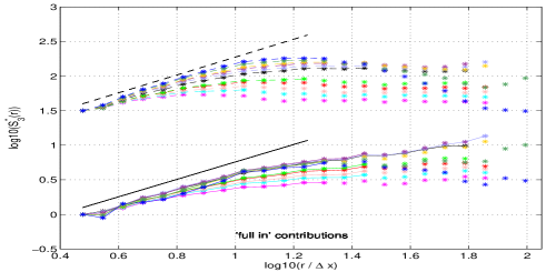
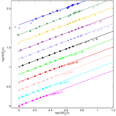
Figure 10: ’Full in’ case for simulations R*_2 at $\ell\approx 12$, color coding as in Fig. 2. Top panel: Structure functions $S_{3}^{\perp}(r)$ (upper curves) and $S_{3}^{\parallel}(r)$ (lower curves), curves vertically shifted to start from one common point. Stars connected by lines indicate data used to determine ESS scaling exponents. Also indicated are slopes $\zeta_{3}^{\parallel}=1.26$ and $\zeta_{3}^{\perp}=1.29$ as obtained by Kritsuk et al. (2007a) for 3D periodic box simulations. Bottom panel: Fit (solid lines) of ESS scaling exponent $Z_{2}^{\parallel}$ as slope of $\mathrm{log10}(S_{2}^{\parallel})$ versus $\mathrm{log10}(S_{3}^{\parallel})$. Filled symbols denote data used for the fit, empty symbols denote all data available.

Table 2: Longitudinal (top) and transverse (middle) ESS scaling exponents $Z_{p}$ and best estimates for co-dimension $C$, case ’full in’ for the different runs at $\ell\approx 12$. Dashes indicate fits of insufficient quality. Also given (bottom) are some analytical values following Eq. 20.

	$p=1$	$p=2$	$p=4$	$p=5$	$C$
R2_2	0.41	0.73	1.20	-	-
R4_2	0.45	0.78	1.14	-	-
R5_2	0.42	0.74	1.15	1.28	0.8
R7_2	0.43	0.76	1.20	1.37	0.9
R8_2	0.44	0.75	1.22	1.42	1.0
R11_2	0.44	0.76	1.21	1.41	1.0
R16_2	0.45	0.76	1.20	1.38	0.9
R22_2	0.43	0.75	1.21	1.41	1.0
R27_2	0.44	0.78	1.23	1.44	1.1
R33_2	0.42	0.77	1.23	1.48	1.2
R43_2	0.44	0.76	1.20	1.50	1.2
R2_2	0.43	0.75	1.23	1.48	1.2
R4_2	0.45	0.76	1.20	1.39	0.9
R5_2	0.46	0.78	1.18	1.34	0.8
R7_2	0.48	0.79	1.17	1.32	0.8
R8_2	0.49	0.80	1.16	1.30	0.8
R11_2	0.52	0.82	1.13	1.26	0.7
R16_2	0.53	0.82	1.12	1.22	0.5
R22_2	0.52	0.81	1.14	1.26	0.7
R27_2	0.52	0.81	1.14	1.25	0.5
R33_2	0.52	0.81	1.14	1.24	0.5
R43_2	-	-	-	-	-
-	0.56	0.83	1.13	1.25	0.7
-	0.47	0.78	1.17	1.32	0.8
-	0.44	0.76	1.20	1.36	0.9
-	0.42	0.74	1.21	1.40	1.0
-	0.41	0.73	1.23	1.42	1.1
-	0.40	0.72	1.24	1.45	1.2

3.4.4 CDL structure functions: beyond the ’full in’ case

The CDL being not strictly periodic and its turbulence asymmetric and inhomogeneous, structure functions are expected to depend on how the averages in Eq. 18 are taken. Apart from the ’full in’ case presented above, we looked at three more cases: ’unified’ and LOSs parallel and perpendicular to the upstream flows (see Sect. 3.4.2). For the perpendicular LOS we tested that results do not depend on whether the y- or z-direction is analyzed, thus only the y-direction is shown. Third order structure functions are shown in Fig. 11, ESS scaling exponents are given in Table 4.

The ’unified’ case by and large resembles the ’full in’ case. The structure functions look similar (Figs. 10 and 11, top panel), the quality of ESS fits is comparable (Fig. 14, columns one and two). Co-dimensions tend to be smaller in the ’unified’ case ($0.9\leq C\leq 0.4$), indicating a dimension $D>2$ for the most dissipating structures. This seems plausible as the ’unified’ case covers the CDL more completely than the ’full in’ case, especially with regard to the highly compressible regions close to the confining shocks. As in the ’full in’ case, there is a tendency of the co-dimension of longitudinal (transverse) structure functions to increase (decrease) with increasing $M_{\mathrm{u}}$.

Structure functions taken along a LOS parallel or perpendicular to the upstream flow look widely different among themselves (Fig. 11, middle and bottom panel) and with respect to both the ’unified’ and ’full in’ case. First, the spread induced by $M_{\mathrm{u}}$ is larger for the perpendicular LOS than for the parallel LOS. We speculate that this may be related to our demand that a ray must not re-enter the CDL (see Sect. 3.4.2), which gains relevance as $M_{\mathrm{u}}$ increases, and implies that regions close to the confining shocks tend to be neglected as $r$ increases. Second, longitudinal structure functions from a parallel LOS do not level off but keep increasing over the distance considered. This seems plausible as with increasing distance the velocity difference in Eq. 18 approaches the difference between the two post shock flow velocities at each of the confining shocks.

Best ESS fits are of reasonable quality for transverse structure functions and low to intermediate $M_{\mathrm{u}}$ (Fig. 14). The concrete values of ESS scaling exponents given in Table 4 (middle and right columns) reveal the crucial role of the orientation of the LOS with respect to the upstream flow: transverse ESS scaling exponents indicate co-dimensions $C>1$ for a LOS parallel to the upstream flow and $C<1$ for a perpendicular LOS. For a parallel LOS there is again a tendency toward smaller co-dimension with increasing $M_{\mathrm{u}}$.

Best ESS fits for the longitudinal structure functions are typically of mediocre quality and difficult to interpret. While we give the corresponding data in the appendix (Table 4), we renounce at their discussion. We only mention two features whose further analysis may be of interest, but is beyond the scope of the present paper. First, for the parallel LOS best fits are typically obtained at intermediate values of $\mathrm{log10}(S^{\parallel}_{\mathrm{3}})$ (Fig. 14, top row, third panel), which translates to intermediate values of $r$. Second, for perpendicular LOSs there is a steeper (shallower) linear slope for larger (smaller) values of $\mathrm{log10}(S^{\parallel}_{\mathrm{3}})$ (Fig. 14, top row, fourth panel). As $M_{\mathrm{u}}$ increases, the shallower slope gradually vanishes and only the steeper slope prevails.

In summary, our results indicate that the LOS plays a crucial role for the CDL structure functions and derived quantities, notably the co-dimension $C$.

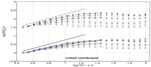
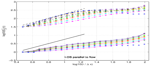
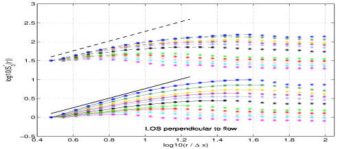
Figure 11: Structure functions $S_{3}^{\parallel}(r)$ (solid) and $S_{3}^{\perp}(r)$ (dashed) for the case ’unified’ (top panel), as well as computed along the x-direction (middle panel) and y-direction (bottom panel), i.e., parallel and perpendicular to the upstream flow, for simulations R*_2 at $\ell=12$. Color coding as in Fig. 2. Also indicated are slopes $\zeta_{3}^{\parallel}=1.26$ and $\zeta_{3}^{\perp}=1.29$ as obtained by Kritsuk et al. (2007a) from 3D periodic box simulations. Curves are vertically shifted, to start from one common point.

3.5 Numerical resolution

It is clear from the literature (e.g., Kritsuk et al., 2007a; Federrath et al., 2010) that the present simulations are at the brink of the necessary resolution to get physically meaningful results in the context of isothermal supersonic turbulence. Computational costs limit concrete numerical resolution studies.

An obvious resolution dependence that can be taken from Table 1, and that was already found for the 2D case (FW06), is that lower resolution results in higher $M_{\mathrm{rms}}$ for the same $M_{\mathrm{u}}$ and for the same CDL size ($\ell\approx 12$). This although there is a tendency toward smaller driving efficiencies (thus less energy input into the CDL) at lower resolutions. We can only speculate about potential reasons for this observed behavior, as to why we find higher resolution to result in lower $M_{\mathrm{rms}}$ (and not higher $M_{\mathrm{rms}}$, as in the subsonic case), despite increased energy input.

One potential explanation we can think of, and which we put forward already in the 2D case: in supersonic turbulence dissipation is dominated by shocks and with increasing resolution more shocks are resolved, thus dissipation increases, thus $M_{\mathrm{rms}}$ decreases. This mechanism we would expect to act primarily on the parallel flow component, as only $M_{\mathrm{rms,\parallel}}>>1$.

Another possible explanation that comes to mind could be that finer resolution tends to promote coupling of parallel and transverse directions. The latter thus may be exploited more efficiently for energy dissipation, predominantly viscous dissipation as $M_{\mathrm{rms,\perp}}<1$. Total energy dissipation (parallel plus transverse directions) thus may increase with increasing resolution. Further potential explanations may exist.

The first idea, enhanced dissipation in shocks, is attractive as it acts predominantly on $M_{\mathrm{rms,\parallel}}$, which dominates $M_{\mathrm{rms}}$ by far. The second idea, enhanced viscous dissipation in transverse directions, fits well with our data in that $M_{\mathrm{rms,\parallel}}/M_{\mathrm{rms,\perp}}$ decreases with increasing resolution, indicating better coupling of transverse and parallel directions. Within the frame of our model set up it is not easy to proof that any of these two ideas are indeed at work, admittedly leaving us for the time being with an unsatisfying situation.

It would be interesting to check whether a similar dependence of $M_{\mathrm{rms}}$ on resolution exists for driven turbulence in 3D periodic box simulations. This could be done by monitoring the amount of energy that has to be injected to maintain a prescribed level of $M_{\mathrm{rms}}$. If the first of the above potential explanations were true, we would expect that for higher resolution more energy has to be injected per time to maintain a prescribed level of turbulence. By contrast, the second of the above potential explanations may hardly manifest itself in the 3D periodic box case, as driving there is typically isotropic and thus coupling among directions is less of an issue than in the present study. The authors are not aware of any dedicated study in this direction.

Besides $M_{\mathrm{rms}}$, other quantities show some resolution dependence as well. Clearly increasing with increasing resolution is $\sigma(\rho)/\rho_{\mathrm{m}}$ (last column of Table 1). As $\rho_{\mathrm{m}}$ shows no clear tendency, this increase is an increase in density variance with resolution. The increase of peak densities with increasing resolution is well known (Hennebelle & Audit, 2007; Kitsionas et al., 2009; Federrath et al., 2010) and expected on numerical grounds.

In summary, we expect our results to essentially hold qualitatively but to change somewhat quantitatively if we were to go to higher resolution. In particular, we would expect somewhat lower $M_{\mathrm{rms}}$ for the same $M_{\mathrm{u}}$ and a larger density variance.

4 Discussion

4.1 3D slabs versus 2D slabs

The relevance of dimensionality for head-on supersonic collision of isothermal flows was already pointed out in Sect. 3.1: while compression of the collision zone scales as $\rho_{\mathrm{m}}/\rho_{\mathrm{u}}\propto M_{\mathrm{u}}^{2}$ in 1D, mean densities of the CDL are largely independent of $M_{\mathrm{u}}$ in 2D and 3D. Comparing the 3D numerical results presented here with corresponding 2D results (FW06) further shows that for the same upstream conditions the interaction zone is more turbulent in 3D than in 2D: $M_{\mathrm{rms}}$ is about 25% of $M_{\mathrm{u}}$ in 3D, but only about 20% in 2D. For the same upstream conditions, driving efficiency is considerably higher in 3D than in 2D (see Fig. 12) and the power law dependence of the driving efficiency on the upstream Mach number is steeper: $\beta_{\mathrm{3}}=-0.7$ in 2D but $\beta_{\mathrm{3}}=-1.17$ in 3D.

We attribute the larger driving efficiency in 3D (a larger fraction of the upstream kinetic energy density traverses the confining shocks of the CDL unthermalized) to the different shock geometry. In 2D, with the CDL extending to infinity in z-direction, the confining shocks resemble a corrugated sheet. In 3D, they look more like a cardboard egg wrapping. Regions where the confining shocks are perpendicular to the upstream flow, thus maximum thermalization occurs, are line-like in the 2D case but point-like in the 3D case (see Fig. 1).

Numerical resolution we exclude as an explanation, as 2D simulations for $M_{\mathrm{u}}=22$ and three different resolutions yield a range of $f_{\mathrm{eff}}\in[0.55,0.62]$ (FW06), whereas the corresponding 3D value is $f_{\mathrm{eff}}=0.84$. This for about the same x-extension of the CDL and about the same coverage (up to a factor of two) of this extension in terms of grid cells.

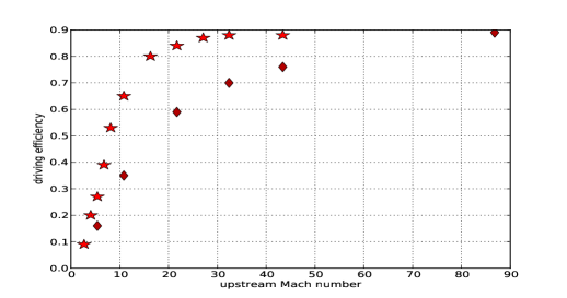
Figure 12: Role of dimensionality for driving efficiency $f_{\mathrm{eff}}$ as function of upstream Mach number $M_{\mathrm{u}}$. Shown are simulations R*_2 (red stars) and corresponding values for 2D slabs (dark red diamonds, simulations R*_0.2.4 in FW06).

4.2 3D slabs versus 3D periodic boxes

The main difference of the simulations presented here to 3D periodic box simulations lies in the driving of the turbulence - and resulting consequences. In 3D periodic box models, energy is typically injected in a controlled, rather homogeneous and isotropic way, although concrete realizations differ. The 3D slab model may be regarded as the other extreme: energy input into the turbulent interaction zone only occurs at the two confining shocks and this in a comparatively uncontrolled way concerning both the amount of energy and the form of the driving (compressible / solenoidal and driving wave length). The kinetic energy flow entering the interaction zone is predominantly directed parallel to the upstream flows. Its absolute amount is modulated by the wiggling of the confining shocks, whose spatial scale in turn correlates with the spatial extension of the interaction zone.

The different forcing is reflected in the character of the turbulence: isotropic, homogeneous, and stationary in the case of 3D periodic box models, anisotropic, inhomogeneous, and with some time evolution for 3D flow collision zones. We even argue (Sect. 3.2.1) that for head-on colliding, isothermal flows it is far from trivial, if not impossible, to reach isotropy while retaining $M_{\mathrm{rms}}>>1$. As a corollary, we see some danger in neglecting the concrete large scale driving of the turbulence and replace it by an isotropic random driving instead. For uniform isothermal, head-on colliding flows as studied here, the anisotropy and inhomogeneity of the turbulence are a direct consequence of the large scale driving. It seems plausible that a similar imprint of the large scales on the small scales is also present in more complex flows, e.g., accretion onto compact objects (Walder et al., 2010). This is not to say that isothermal isotropic supersonic turbulence cannot exist. But we caution that its realization may not be straight forward, at least not in the context of large scale colliding flows.

Density PDFs deviate from log-normal already in 3D periodic box simulations of driven isothermal turbulence if the driving has a substantial compressible component (Schmidt et al., 2009; Federrath et al., 2010). It thus seems plausible that our density PDFs deviate from log-normal. However, the deviations we find are more pronounced than those seen in compressibly forced 3D periodic box simulations. A potential reason could be the inhomogeneity of the turbulence in the collision zone. The more violent turbulence close to the confining shocks may be responsible not only for high compressions but also for pronounced low density voids, as visible in the 2D case, Fig. 1, left panel. Density PDFs for individual 2D slices may shed more light on this issue but were beyond the scope of the present paper. For molecular clouds, if they indeed result from colliding flows, the high-density tail we find suggests that current star formation models based on log-normal density distributions may severely underestimate high mass star formation, even more than already postulated in Schmidt et al. (2009) on the basis of their simulations.

Regarding ESS scaling exponents, Table 3 shows that our values lie well within the range of published values. They basically range from the theoretical model by She & Leveque (1994) ($C=2$) to numerical 3D periodic box results by Schmidt et al. (2009). The very low values for $Z_{4}$ and $Z_{5}$ found in the later study are, however, never reached in our data. Nevertheless, our data are much closer to these values than any other of the listed data.

The range of $Z_{p}$ values we observe results, on the one hand, from the dependence of $Z_{p}$ on $M_{\mathrm{u}}$. The dependence is particularly clear for transverse structure functions. Here, $Z_{2}$ increases with $M_{\mathrm{u}}$, in line with the notion of universal scaling. Longitudinal structure functions show rather inconclusive results in this respect, possibly contradicting expectations from universal scaling. Whether isothermal turbulence, in flow collision zones or 3D periodic box simulations, indeed displays non-universal scaling properties, possibly due to an additional degree of freedom related to the large scale forcing as suggested by Schmidt et al. (2009), remains to be seen.

The other reason for the large range of $Z_{p}$ are LOS effects, a point we take up again in Sect. 4.3.2. Here we only note that parallel and perpendicular LOSs (rows 3 and 4 in Table 3) display nearly complementary ranges in terms of $Z_{p}$, and that it is mainly the parallel LOS which is responsible for $Z_{p}$ values close to theoretical values by She & Leveque (1994). This kind of LOS effects is likely absent in 3D periodic box simulations.

Table 3: Comparing ESS scaling exponents $Z_{p}$, $p=1$ to $p=5$, following Table 4 in Schmidt et al. (2009). Listed are values from this work, for longitudinal ($\parallel$) and transverse ($\perp$) structure functions, simulation data by Boldyrev et al. (2002a) (BNP02), Kritsuk et al. (2007a) (KNPW07), Schmidt et al. (2009) (SFHKN09), and theoretical values by Kolmogorov (1941) (K41), She & Leveque (1994) (SL94), Boldyrev (2002) (B02).

p	1	2	3	4	5
this work, ’full in’ case ($\parallel$)	0.41 - 0.46	0.73 - 0.80	1.00	1.12 - 1.23	1.19 - 1.50
this work, ’full in’ case ($\perp$)	0.43 - 0.53	0.75 - 0.82	1.00	1.13 - 1.23	1.23 - 1.45
this work, perpendicular LOS ($\perp$)	0.42 - 0.51	0.75 - 0.81	1.00	1.14 - 1.20	1.27 - 1.40
this work, parallel LOS ($\perp$)	0.38 - 0.43	0.71 - 0.77	1.00	1.18 - 1.27	1.38 - 1.54
BNP02 (MHD 5003)	0.42	0.74	1.00	1.20	1.38
KNPW07 (HD 10243)	0.43	0.76	1.00
SFHKN09 (HD 7683)	0.52	0.83	1.00	1.09	1.14
K41	0.33	0.67	1.00	1.33	1.67
SL94 ($C=2$)	0.36	0.70	1.00	1.28	1.54
B02 ($C=1$)	0.42	0.74	1.00	1.21	1.40

4.3 Toward real objects?

The physical model examined here is clearly too simple for direct comparison with real world observations. Nevertheless, we consider it worthwhile to contemplate on potential real-world implications of two results, putting them at the same time into perspective by speculating on effects of some neglected physics. Finally, we reverse the perspective and ask for which classes of real objects 3D slab studies may provide useful physical insight.

4.3.1 Driving the turbulence: high $M_{\mathrm{rms}}$, high $M_{\mathrm{u}}$?

The first point we want to discuss more thoroughly is the rather poor conversion from $M_{\mathrm{u}}$ to $M_{\mathrm{rms}}$, the latter being only about 10% to 20% of the former in the core region of the CDL. For molecular clouds, where observations indicate $M_{\mathrm{rsm}}\approx 5-50$ (Zuckerman & Evans, 1974; McKee & Ostriker, 2007; Klessen, 2011; Polychroni et al., 2012), and assuming that molecular clouds result from large scale flow collisions, this would imply $M_{\mathrm{u}}\approx 40-500$ within the frame of our model.

Several questions may be asked. How could such fast flows be produced? Could inclusion of additional physics within the frame of colliding flows improve the conversion from $M_{\mathrm{u}}$ to $M_{\mathrm{rsm}}$? Are driving mechanisms other than colliding flows compelling? We will mostly dwell on the second question.

The inclusion of radiative cooling may or may not improve conversion from $M_{\mathrm{u}}$ to $M_{\mathrm{rsm}}$. Simulations where the cooling limit, and thus the lowest temperature within the CDL, is equal to the upstream flow temperature show less turbulence (smaller $M_{\mathrm{rms}}$) than isothermal simulations with the same upstream Mach number (Walder & Folini, 2000b; Folini et al., 2010). If significant cooling layers form at the confining shocks, the associated large thermal post-shock pressure will tend to straighten the confining shocks. A positive feedback results: the more straight the confining shocks, the more upstream kinetic energy is thermalized at these shocks, the higher the post-shock temperature, the stronger the corresponding thermal pressure and the longer the cooling time for the shock-heated gas. And the less kinetic energy is available for driving the turbulence.

The situation may be different during the very early collision phase, when the CDL is still very thin, and especially if the post shock temperature falls within a temperature range where cooling instabilities occur, i.e., where cooling becomes more and more efficient as the temperature decreases. The early (thin) CDL as a whole becomes very unstable under such conditions (Walder & Folini, 2000b; Heitsch et al., 2005; Folini et al., 2010; Heitsch et al., 2011). The situation may also change if the cooling limit is decidedly below the temperature of the upstream flow (Pittard et al., 2005). The CDL then can cool to temperatures well below the upstream flow temperature, the sound speed within the CDL decreases and, consequently, the Mach number increases. Except for this last possibility, it seems rather unlikely that inclusion of radiative cooling improves the conversion from $M_{\mathrm{u}}$ to $M_{\mathrm{rsm}}$. Isothermal conditions rather set an upper limit.

Other physics of potential relevance for $M_{\mathrm{rms}}$ (and beyond) but not covered by our model include magnetic fields, which may increase the CDL turbulence by additional energy input through reconnection or decrease the turbulence as the field guides the flow direction. More specifically for molecular clouds, inclusion of self-gravity may augment the turbulence within the cloud. MHD waves generated by moving accreting cores may stir the turbulence (Folini et al., 2004). Turbulence may also be driven through jets, winds, and radiation from young or forming stars.

All possibilities just listed to augment $M_{\mathrm{rms}}$ have in common that they drive the turbulence from within the CDL. For molecular clouds this may seem in contradiction with observation based results favoring driving on the scale of the cloud (Ossenkopf & Mac Low, 2002; Heyer et al., 2006; Brunt et al., 2009; Roman-Duval et al., 2011). These results are also somewhat challenging with regard to our findings. For our CDL, the wiggling of the confining shocks modulates the incoming flows. It seems plausible that the spatial scale of this modulation affects, or even sets, the driving scale of the turbulence. If so, this would imply an energy injection scale that is smaller than the CDL size, as the spatial scale of this wiggling is smaller than the spatial extension of the CDL. The scale of the wiggling increases, however, in proportion to the CDL size as the CDL grows (see FW06). Also, our simulations suggest that spatial modulation of the incoming flow comprises not one scale but some continuum of scales.

A speculative solution to the above, somewhat conflicting, results and demands for molecular clouds could be that various driving mechanisms and associated driving wave lengths co-exist: external large scale and internal small scale driving. The latter would add to $M_{\mathrm{rms}}$, thus would help to overcome the poor conversion from $M_{\mathrm{u}}$ to $M_{\mathrm{rms}}$ and the associated demand for very high Mach number flows. It also would help to make the turbulence more isotropic, something we have shown is difficult to achieve within the frame of isothermal colliding flows. Large scale forcing would equally add to $M_{\mathrm{rms}}$ and leave a characteristic large-scale-driving imprint in the turbulence.

4.3.2 Viewing angle effects?

The second finding that in our opinion deserves discussion is the strong anisotropy of CDL velocities. It means that line-of-sight velocities of an observer, and any derived quantities, will depend on the viewing angle of the CDL. The same CDL can display supersonic or subsonic line-of-sight velocities, depending on whether the line-of-sight of the observer is oriented parallel or perpendicular to the incoming flows. The density Mach number relation suffers from the same problem. If taken as indicative of the nature of the driving ($b=1/3$ for solenoidal driving and $b=1$ for compressible driving, from isothermal 3D periodic box simulations, see Federrath et al. (2008)), the viewing angle will co-decide whether one concludes for the same CDL that its driving is rather compressible or solenoidal.

Equally affected are ESS scaling exponents $Z_{p}$. For transverse structure functions and derived co-dimensions we have shown that results depend crucially on the adopted viewing angle: co-dimensions $C>1$ ($C<1$) are obtained for a line-of-sight parallel (perpendicular) to the upstream flow. As stressed before, these results are preliminary in that they do not take into account radiative transfer, density effects, or projection effects. That such factors matter is well established in the literature (Stutzki et al., 1998; Brunt & Mac Low, 2004; Sánchez et al., 2005; Ossenkopf et al., 2006; Esquivel et al., 2007; Brunt et al., 2009; Federrath et al., 2010). Further analysis of our data in this direction is envisaged but beyond the scope of the present paper.

Despite this cautionary remark, it is tempting to dwell a moment longer on the subject and add a concrete illustration of our point that line-of-sight effects should be considered as one more factor when interpreting observational data. As an example, consider simulation R5_2, whose transverse structure functions are generally well behaved. In terms of $Z_{p}$ we find $Z_{1}=0.38$ and $Z_{5}=1.49$ when looking at the CDL parallel to the upstream flow, but $Z_{1}=0.45$ and $Z_{5}=1.37$ when the line-of-sight is perpendicular to the upstream flow. In the first case, with values roughly similar to observation based results for the Polaris Flare (Hily-Blant et al., 2008), we deduce a co-dimension of $C=1.5$ and may conclude that the forcing is predominantly solenoidal and, possibly, that the turbulence is not too compressible. If we look at the same data but from a different viewing angle, now perpendicular to the upstream flow, we deduce a co-dimension of $C=0.9$ and may conclude that the turbulence is highly compressible and the forcing rather compressible than solenoidal.

4.3.3 3D slabs: a useful concept for real objects?

In a number of astrophysical objects, large scale colliding flows play a key role, i.e., flows with a dominant bulk velocity component on top of any additional flow structure. In fact, the present study was motivated by numerical simulations of entire objects by the authors (Folini & Walder, 2000; Dumm et al., 2000; Folini & Walder, 2002; Harper et al., 2005; Walder et al., 2005, 2008; Georgy et al., 2013). We advocate that insight into the physics of such collision zones can be gained from 3D slab studies. The present study, for example, shows that a richly structured interaction zone exists even for rather simple physics and although the colliding flows are essentially reduced to their bulk properties. Of course, real colliding flows likely harbor more structure and physics. The relative importance of such additional complexity may be gradually addressed within the context of 3D slabs.

Taking the perspective of astrophysical objects, 3D slab studies may be useful for the wind collision zone in massive binaries. Concrete questions range from the X-ray and non-thermal emission of such zones (e.g., Pittard & Parkin, 2010; Zhekov, 2012; De Becker & Rauw, 2013) to dust formation near periastron passage, presumably in the collision zone and despite the strong stellar radiation fields (Tuthill et al., 1999; Marchenko et al., 1999; Cherchneff et al., 2000; Folini & Walder, 2002; Dougherty et al., 2005; Williams et al., 2012). Such studies clearly require more physics than covered in this paper. Also, massive stellar winds are likely clumped (e.g., Owocki et al., 1988; Moffat et al., 1988), which can affect the turbulence in the collision zone (e.g., Walder & Folini, 2002; Pittard, 2007; Pittard et al., 2009, 2010). Another large class of objects where 3D slabs might provide some insight are internal collisions in jets, from young stars (e.g., Flower et al., 2003; Cunningham et al., 2006, 2011) to high-energy objects, like gamma ray burst (Mimica et al., 2007; Zitouni et al., 2008; Bošnjak et al., 2009; Mimica & Aloy, 2010; Granot, 2012). In the later case, however, relativistic effects are likely relevant. A third context where 3D slab studies might be useful is star formation on galactic scales. Turbulence in the wake of flow collision is one suggested explanation (e.g., Gabor & Bournaud, 2013) for the observed delay and potential suppression of star formation for $z>2$ (e.g., Bouché et al., 2010; Weinmann et al., 2012). The case of 3D slabs and molecular clouds we briefly touched in Sect. 4.3.1. A multi-phase medium is likely relevant for such studies (e.g., Hennebelle & Pérault, 1999; Hennebelle et al., 2007; Gray & Scannapieco, 2013). Also, the flows probably already carry (turbulent) structure, whose effect on the collision zone remains to be clarified. In fact, we consider it a most interesting question whether gradual inclusion of such and other effects allows to recover the 3D periodic box view on molecular cloud turbulence (see Sect. 4.2) in the context of 3D slabs. We are not aware of any such studies.

5 Summary and conclusions

We have performed 3D simulations of head-on colliding isothermal flows with upstream Mach numbers in the range $2\leq M_{\mathrm{u}}\leq 43$ and presented a first analysis of the turbulence in the resulting interaction zone, the CDL (cold dense layer). We find that the characteristics of the CDL turbulence deviate markedly from what is obtain in corresponding 3D periodic box simulations.

As in 2D, approximate self-similar scaling relations also hold in 3D for the mean density, root mean square Mach number, driving efficiency, and energy dissipation in the CDL, albeit with different numerical constants and a different (steeper) scaling exponent for the driving efficiency. For the same $M_{\mathrm{u}}$, the driving efficiency is larger in 3D than in 2D because of the different shock geometry (’egg wrapping’ in 3D, ’corrugated sheet’ in 2D).

Density PDFs are not log-normal but show fat tails at high densities and a ’two-power-law’ composite for low densities.

The CDL turbulence is inhomogeneous and anisotropic. Root mean square Mach numbers are around 15% (CDL center) to 25% (CDL average) of $M_{\mathrm{u}}$. They are always larger parallel to the upstream flow than in perpendicular direction, where they never reach supersonic values. The density variance - Mach number relation inherits this anisotropy. Isotropization of the flow hardly takes place and we argue, in fact, that isotropization is hard to achieve while retaining substantially supersonic root mean square Mach numbers. Even in the (small scale) central region of the CDL the turbulence remains anisotropic, even here the imprint of the large scale driving is still felt.

The viewing angle of the CDL is shown to play a prominent role for different turbulence characteristics like ESS scaling exponents or the density variance - Mach number dependence. ESS scaling exponents of transverse structure functions imply for the most dissipative structures a dimension $D<2$ if computed for a line-of-sight parallel to the upstream flow, but $D>2$ if taken along a line-of-sight perpendicular to the upstream flow. We suggest to keep this in mind when interpreting observational data.

Our results show that even our very simple model setup results in a very richly structured, turbulent interaction zone. The physical system studied thus opens a perspective on supersonic turbulence that is rewarding and complementary to 3D periodic box simulations. Under what conditions both perspectives may be united we consider an interesting question for the future. The finite size of the interaction zone is a challenge with regard to data analysis and interpretation of results. But this finite size makes the data also potentially very interesting, as real objects are of finite size as well, and therefore likely incorporate boundary effects. Moreover, bulk flows in real astrophysical objects likely carry some structure (are inhomogeneous) and require a more elaborate physical description than the isothermal approach taken here. The assumption of head-on collision equally needs to be relaxed and the role of numerical resolution for supersonic turbulence needs investigation. The robustness of our findings against these factors remains to be tested. Nevertheless, we consider the present study a useful contribution for the physical understanding of complex real objects.

Appendix A Derivation of analytical expression for the driving efficiency

Part of the total (left plus right) upwind kinetic energy flux density, ${\cal F}_{\mathrm{e_{\mathrm{kin}},u}}=\rho_{\mathrm{u}}v_{\mathrm{u}}^{3}$, is thermalized at the shocks confining the CDL. The remaining part, $\dot{\cal E}_{\mathrm{drv}}$, drives the turbulence in the CDL. In analogy with the 2D case, we assume that $\dot{\cal E}_{\mathrm{drv}}$ and ${\cal F}_{\mathrm{e_{\mathrm{kin}},u}}$ are related by a function of the upwind Mach-number alone,

$$\dot{\cal E}_{\mathrm{drv}}=f_{\mathrm{eff}}(M_{\mathrm{u}}){\cal F}_{\mathrm{e_{\mathrm{kin}},u}}.$$ (22)

We call the function $f_{\mathrm{eff}}$ the driving efficiency. An expression for $f_{\mathrm{eff}}$ can be derived by using the jump conditions for strong, oblique shocks,

$$\rho_{\mathrm{d}} = \rho_{\mathrm{u}}M_{\mathrm{\perp,u}}^{2}=\rho_{\mathrm{u}}M_{\mathrm{u}}^{2}\cos^{2}\alpha,$$

$$v_{\mathrm{\perp,d}} = v_{\mathrm{\perp,u}}M_{\mathrm{\perp,u}}^{-2}=\frac{a}{M_{\mathrm{u}}\cos\alpha},$$

$$v_{\mathrm{\parallel,d}} = v_{\mathrm{\parallel,u}}=aM_{\mathrm{u}}\sin\alpha.$$ (23)

The subscript d denotes downstream quantities, right after shock passage, the subscripts ${\mathrm{\perp}}$ and ${\mathrm{\parallel}}$ denote flow components perpendicular and parallel to the shock, and $\alpha$ is the absolute value of the angle between the x-axis and the normal to the shock. Using Eq. 23 we obtain

$$\dot{\cal E}_{\mathrm{drv}} = \frac{1}{YZ}\int_{S_{\mathrm{l,r}}}ds\frac{\rho_{\mathrm{d}}v_{\mathrm{d}}^{2}}{2}v_{\mathrm{\perp,d}}$$ (24)

$$= \frac{1}{YZ}\int_{S_{\mathrm{l,r}}}ds\frac{\rho_{\mathrm{u}}M_{\mathrm{\perp,u}}^{2}(v_{\mathrm{\parallel,u}}^{2}+v_{\mathrm{\perp,u}}^{2}M_{\mathrm{\perp,u}}^{-4})}{2}v_{\mathrm{\perp,u}}M_{\mathrm{\perp,u}}^{-2}$$

$$\approx \frac{1}{YZ}\int_{S_{\mathrm{l,r}}}ds\frac{\rho_{\mathrm{u}}v_{\mathrm{\parallel,u}}^{2}}{2}v_{\mathrm{\perp,u}}$$

$$= \frac{\rho_{\mathrm{u}}v_{\mathrm{u}}^{3}}{2YZ}\int_{S_{\mathrm{l,r}}}ds\cos(\alpha)(1-\cos^{2}(\alpha))$$

$$= \frac{\rho_{\mathrm{u}}v_{\mathrm{u}}^{3}}{2YZ}\int_{YZ_{\mathrm{l,r}}}dydz(1-\cos^{2}(\alpha)),$$ (25)

where the integrals over $S_{\mathrm{l,r}}$ and $YZ_{\mathrm{l,r}}$ run over the left and right shock and where it was used that $ds\cos(\alpha)=dydz$. We further used the shock jump conditions given in Eq. 23, that $v_{\mathrm{d}}^{2}=v_{\mathrm{\parallel,d}}^{2}+v_{\mathrm{\perp,d}}^{2}$, and that $v_{\mathrm{\parallel,u}}^{2}=v_{\mathrm{u}}^{2}(1-\cos^{2}(\alpha))$. The term $M_{\mathrm{\perp,u}}^{-4}$ is omitted as the shocks we observe in our simulations fulfill $\cos\alpha>>M_{\mathrm{u}}^{-2}$ for the most part. Analogous to the 2D case we thus obtain

$$f_{\mathrm{eff}}=\frac{1}{2YZ}\int_{Y_{\mathrm{l,r}}}dydz(1-\cos^{2}(\alpha))\equiv 1-\cos^{2}(\alpha_{\mathrm{eff}}),$$ (26)

where we used the midpoint rule.

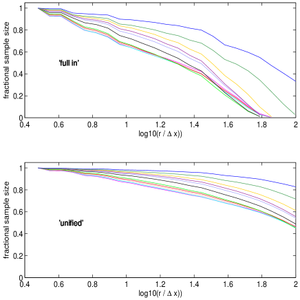
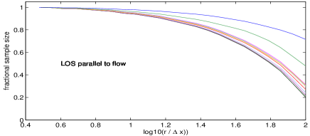
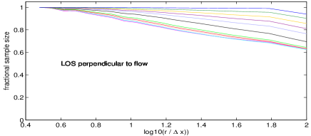
Figure 13: Sample size versus radial distance, normalized to the sample size at the smallest radius for cases ’full in’ (first panel), ’unified’ (second panel), parallel LOS (third panel), and perpendicular LOS (fourth panel) for the different runs, all at $\ell\approx 12$. Color coding as in Fig. 2.

Appendix B Structure functions from CDL data: computational details and additional results

B.1 Computing structure functions from CDL data

To compute $S_{p}(r)$ from our slab data, we consider data of only one time step, at $\ell\approx 12$. To average over all positions $\mathbf{x}$, we step through all grid points in the CDL. To average over all directed distances $\mathbf{r}$, we cast rays at each position $\mathbf{x}$ into 20 directions, given by the surface normals of an icosahedron centered at $\mathbf{x}$: $(\pm 1,\pm 1,\pm 1)$, $(0,\pm 1/\varphi,\pm\varphi)$, $(\pm 1/\varphi,\pm\varphi,0)$, and $(\pm\varphi,0,\pm 1/\varphi)$ with $\varphi=(1+\sqrt{5})/2$. We tested the robustness of our results against rotation of this icosahedron. We step along each ray and compute the longitudinal and transverse contribution to $S_{p}(r)$. Each ray is covered by 23 logarithmically spaced steps from 3 $\Delta x$ to 100 $\Delta x$, $\Delta x$ being the grid cell size. Much larger distances (beyond 128) make no sense because of the periodic domain. Only points within the CDL may contribute to $S_{p}(r)$. A ray that once left the CDL is forbidden to re-enter the CDL at a larger $r$.

As for a given position $\mathbf{x}$ and distance $r$ some rays may already reach outside the CDL while others still lie within, we distinguish two cases for each pair ($\mathbf{x}$, $r$): all 20 rays are still within the CDL (’full in’ case) or at least one ray has left the CDL (’some out’ case). The ’full in’ case ascertains that only symmetric contributions (all 20 directions) enter the mean in Eq. 18. The price to pay is a rather rapidly decreasing and non-uniform sample size: only points $\mathbf{x}$ close to the center of the CDL contribute to $S_{p}(r)$ for large $r$. Considering ’full in’ and ’some out’ contributions in the mean in Eq. 18 (’unified’ case) samples the CDL as completely as possible, but introduces some asymmetry in the computation of the mean in Eq. 18: some directions are missing for some $\mathbf{x}$ and $r$, especially for large $r$. The different sample sizes as function of distance $r$ are illustrated in Fig. 13. Third order structure functions are shown in Figs. 10 and 11.

While structure functions based on spherical averaging are of theoretical interest, observation based structure functions are necessarily based on line-of-sight data. This motivated us to compute structure functions also along individual one dimensional directions, parallel or perpendicular to the upstream flow. The direction of computation may be interpreted as a line-of-sight (LOS), although we stress that no density variations or radiative transfer effects are taken into account. Also, our demand that a ray having left the CDL may not re-enter it, implies for perpendicular LOSs that regions close to the (wiggled) confining shocks contribute to $S_{p}(r)$ only for small $r$, whereas large distances are dominated again by contributions from the central part of the CDL. For a parallel LOS, the velocity difference in Eq. 18 approaches, as $r$ increases, the difference between the two post shock flow velocities at each of the confining shocks.

B.2 Computation of ESS scaling exponents

Given the small inertial range of our structure functions, apparent in Fig. 10, top panel, we make use of the ESS hypothesis and compute linear fits to $Z_{p}$, i.e., to $\mathrm{log10}(S_{p})$ versus $\mathrm{log10}(S_{3})$. We restrict the analysis to distances where the third order structure functions still increase, i.e., we demand that $\mathrm{log10}(S_{3}(r_{i}))>0.99\,\mathrm{log10}(S_{3}(r_{i-1}))$ for $i>4$. We further require that at least eight data points enter the linear fit (corresponding to roughly half a magnitude in $r$). Within these limits, we search for the best linear fit (of $Z_{p}$) in terms of relative standard error. Finally, we reject even the best fit if its relative standard error exceeds 5%. While the choice of 5% is arbitrary, we found the results to remain essentially unchanged if we repeated the analysis with a value of 10%. For the ’full in’ case, the quality of the fits is illustrated in Fig. 10, bottom panel, for longitudinal structure functions and $p=2$. In appendix B, the quality of the fits is illustrated for all cases considered (’full in’, ’unified’, different LOSs) for $Z_{5}$ (Fig. 14). From $Z_{p}$, $p=1$ to $5$, and Eq. 20 a best estimate for the co-dimension $C$ is derived for each run (minimal RMS error). Note that typically more than the required 8 points enter each ESS fit and that the best fit is found for the smallest distances $r$. This situation is typical for nearly all the situations considered. The only exceptions are ESS for longitudinal structure functions computed along one dimensional line-of-sights (see Sect. 3.4.4).

B.3 ESS scaling exponents, beyond the ’full in’ case

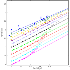
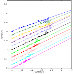
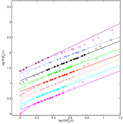
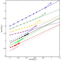
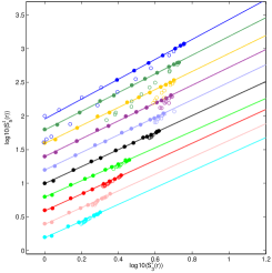
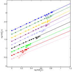
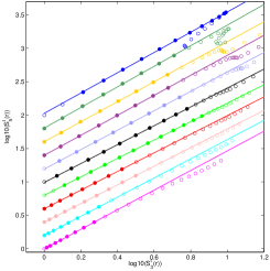
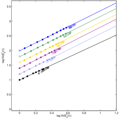
Figure 14: Fits (solid lines) of ESS scaling exponents $Z_{5}$ as the slope of $\mathrm{log10}(S_{5})$ versus $\mathrm{log10}(S_{3})$ for longitudinal (top row) and transverse (bottom row) structure functions for the cases ’full in’ (first column), ’unified’ (second column), parallel LOS (third column), and perpendicular LOS (fourth column). Filled symbols denote data used for the fit, empty symbols denote all data available. Color coding as in Fig. 2.

Table 4: Longitudinal (top) and transverse (bottom) ESS exponents $Z_{p}$ and best estimates for co-dimension $C$ for the case ’unified’ (left columns) and line-of-sights parallel (middle columns) and perpendicular (right columns) to the upstream flow, for the different runs at $\ell\approx 12$. Dashes indicate that no fit of sufficient quality could be obtained.

	’unified’						’parallel to upstream flow’						’perpendicular to upstream flow’
	p=1	p=2	p=4	p=5	$C$		p=1	p=2	p=4	p=5	$C$		p=1	p=2	p=4	p=5	$C$
R2_2	0.59	0.93	0.97	0.95	0.6		-	-	-	-	-		0.39	0.72	1.23	1.42	1.1
R4_2	0.56	0.89	1.02	1.03	0.6		-	-	-	-	-		0.42	0.77	1.10	1.09	0.5
R5_2	0.55	0.88	1.04	1.07	0.6		-	-	-	-	-		0.46	0.82	0.97	0.80	0.3
R7_2	0.51	0.83	1.11	1.22	0.5		0.68	0.94	0.98	1.29	0.6		0.47	0.74	0.94	0.72	0.5
R8_2	0.49	0.80	1.14	1.26	0.8		0.62	0.90	1.02	1.00	0.3		0.39	0.72	1.22	1.46	1.2
R11_2	0.50	0.81	1.15	1.27	0.8		0.60	0.88	1.05	1.08	0.6		0.40	0.73	1.21	1.37	1.0
R16_2	0.51	0.81	1.16	1.29	0.8		0.61	0.89	1.04	1.00	0.3		0.43	0.76	1.23	1.54	1.7
R22_2	0.52	0.81	1.16	1.31	0.8		0.61	0.89	1.04	1.02	0.3		0.40	0.73	1.18	1.29	0.9
R27_2	0.51	0.81	1.18	1.34	0.8		0.60	0.88	1.04	1.05	0.6		0.37	0.71	1.23	-	-
R33_2	0.50	0.80	1.16	1.34	0.8		0.58	0.87	1.05	1.05	0.6		-	-	-	-	-
R43_2	0.48	0.78	1.18	1.38	0.9		0.56	0.86	1.05	1.06	0.6		-	-	-	-	-
R2_2	0.47	0.78	1.15	1.27	0.8		0.38	0.74	1.26	1.52	1.6		0.42	0.75	1.20	1.36	0.9
R4_2	0.48	0.79	1.16	1.29	0.8		0.38	0.71	1.27	1.54	1.9		0.44	0.76	1.20	1.37	0.9
R5_2	0.49	0.80	1.15	1.28	0.8		0.38	0.71	1.26	1.49	1.5		0.45	0.77	1.19	1.37	0.9
R7_2	0.49	0.80	1.17	1.32	0.8		0.38	0.71	1.26	1.49	1.5		0.45	0.77	1.20	1.40	0.9
R8_2	0.50	0.80	1.16	1.31	0.8		0.39	0.72	1.24	1.45	1.2		0.47	0.77	1.19	1.37	0.9
R11_2	0.53	0.82	1.13	1.24	0.5		0.42	0.74	1.22	1.41	1.0		0.51	0.81	1.14	1.27	0.7
R16_2	0.57	0.85	1.10	1.19	0.4		0.42	0.75	1.20	1.38	1.0		-	-	-	-	-
R22_2	0.58	0.86	1.09	1.15	0.6		0.43	0.75	1.21	1.39	1.0		-	-	-	-	-
R27_2	0.59	0.87	1.08	1.13	0.6		0.42	0.75	1.21	1.39	1.0		-	-	-	-	-
R33_2	-	-	-	-	-		0.43	0.75	1.18	1.43	1.0		-	-	-	-	-
R43_2	-	-	-	-	-		0.44	0.77	1.26	1.47	1.2		-	-	-	-	-