Warm dense matter conductivity including electron-electron collisions

Abstract

We present an approach that can resolve the controversy with respect to the role of electron-electron collisions in calculating the dynamic conductivity of dense plasmas. In particular, the dc conductivity is analyzed in the low-density, non-degenerate limit where the Spitzer theory is valid and electron-electron collisions lead to the well-known reduction in comparison to the result considering only electron-ion collisions (Lorentz model). With increasing degeneracy, the contribution of electron-electron collisions to the dc conductivity is decreasing and can be neglected for the liquid metal domain where the Ziman theory is applicable. We give expressions for the effect of electron-electron collisions in calculating the conductivity in the warm dense matter region, i.e. for strongly coupled Coulomb systems at arbitrary degeneracy.

I Introduction

Physical properties of warm dense matter (WDM) have become an emerging field of research. New techniques such as intense ultra-short pulse laser irradiation or shock wave compression allow to produce states of matter with high energy density in the laboratory that are of relevance for astrophysical processes. In the density-temperature plane of Coulomb systems, the region of degenerate, strongly coupled plasmas is now accessible.

The calculation of properties of WDM is a challenging task. Transport properties, in particular the dc conductivity, are well investigated for a fully ionized plasma in the classical, low-density limit as given by Spitzer and Härm Spitzer53 within kinetic theory (KT), see also Brantov08 and references given there in. The evolution of the electron velocity distribution function is described by a Fokker-Planck kinetic equation. The linearized kinetic equations are solved with a Landau collision integral, that includes both the electron-ion ($e-i$) and electron-electron ($e-e$) collisions.

Alternatively, the conductivity of strongly degenerate electron systems such as liquid metals has been obtained by Ziman and Faber Ziman using the relaxation time approach. The treatment of $e-i$ interaction has been improved by Dharma-wardana dharma06 and others Appel62 ; RH82 ; Chatto81 who used expressions for the pseudo-potentials and ionic structure factors that are appropriate for the particular ions under consideration. Lee and More LeeMore extended this approach to the non-degenerate regime. Desjarlais MPD-LM later derived corrections to the Lee-More conductivity model due to partial ionization. However, to recover the Spitzer result for the conductivity, $e-e$ collisions have to be taken into account. This is not consistently possible within the relaxation time approach Appel61 , but has been done by Stygar stygar02 and Fortov et al.  Fortov03 using interpolation procedures, see also Adams et al.  Adams07 . In this work, we present a general approach using linear response theory (LRT) that allows also for a systematic treatment of $e-e$ collisions at arbitrary degeneracy.

The investigation of time-dependent fields is somehow difficult in KT, too. Often, the collision term in the time dependent kinetic equation is replaced by an energy dependent but static relaxation time ansatz, see Landau and Lifshits landau10 , Dharma-wardana dharma06 , or Kurilenko et al.  Berk92 ; Kuri95 . According to Landau and Lifshits landau10 it should be emphasized that such an approach is only applicable in the low-frequency limit. The high-frequency region, relevant for describing bremsstrahlung, can be treated in LRT, see Reinholz12 . In the present work, we focus on the static conductivity for a response to an electric field that is constant in time and space (dc conductivity).

Recently, the Kubo-Greenwood formula Kubo66 ; Greenwood was considered as a promising approach to the dynamical conductivity in dense, strongly interacting systems at arbitrary degeneracy. Based on the rich experience in electronic structure calculations for solids, liquids and complex molecules using density functional theory (DFT) and the enormous progress in computing power, ab initio simulation techniques have been developed that allow to treat a large number of constituents with individual atomic structure. Most successful so far has been a combination of DFT for the electron system and classical molecular dynamics (MD) simulations for the ions which we will refer to as the DFT-MD method in what follows; for details, see Desjarlais02 ; Mazevet05 ; holst08 ; Holst11 . This method does not rely on effective pair potentials or two-particle cross sections as in standard KT which become questionable in dense, strongly coupled plasmas. The evaluation of the Kubo-Greenwood formula using optimal single electron states gives the full account of $e-i$ interaction and treats $e-e$ interactions based on the exchange-correlation (XC) functional used in the DFT cycle. The inclusion of $e-e$ collisions into the DFT-MD calculations of transport properties in WDM is a subject of lively debate, especially for the limiting case of non-degeneracy.

Within this paper, we apply a generalized approach to non-equilibrium processes according to Zubarev et al.  ZMR2 ; Roepke13 . Using this generalized linear response theory (gLRT) transport properties are related to equilibrium correlation functions such as current-current or force-force correlation functions. Different expressions for the conductivity are deduced which lead to identical results should they be calculated exactly, as was shown analytically by performing partial integration. However, they are differently suited for performing calculations after perturbation expansions. In particular, expressions that are consistent with KT (Spitzer result for the dc plasma conductivity) are compared with the Ziman-Faber theory, the Kubo-Greenwood formula, and the rigorous results for the Lorentz model. In the Lorentz model, non-interacting electrons are considered to move under the influence of the potential of the ions at given configuration (adiabatic limit).

Transport theory for WDM benefits from different sources. On one hand, the conductivity of liquid metals and disordered solids is well described in the weak scattering limit (Fermi’s golden rule) by the Ziman formula if the conducting electrons are degenerate, see also the Ziman-Faber approach Ziman where alloys at finite temperatures are considered ChrisRoep85 . Main ingredients are the element-specific electron-ion pseudo-potential and the (dynamical) ion structure factor that are adequately described using the Kubo-Greenwood formula where the $e-i$ and the $e-e$ interaction (via the XC functional) are considered in any order. Evaluating the correlation functions within DFT-MD Desjarlais02 ; Mazevet05 ; holst08 ; Holst11 no perturbation expansion is performed. On the other hand, the conductivity of plasmas is described by KT so that in the low-density, non-degenerate limit the Coulomb interaction between $e-i$ as well as $e-e$ pairs leads to the Spitzer result. At higher densities, gLRT can be applied that considers correlation functions to be evaluated analytically using the method of thermodynamic Green functions Roep88 ; Berk93a ; rerrw99 ; Roepke13 ; RRN95 . Non-perturbative solutions are possible by classical MD simulations using effective pair potentials, see Igor05 , as long as the non-degenerate case is considered.

Bridging between both, the transport theory of condensed matter and plasma kinetic theory, the contribution of $e-e$ collisions that is clear in KT remains unclear in the Ziman or Kubo-Greenwood approach dharma06 . We address this problem within gLRT that incorporates the Kubo formula as well as the KT as particular special cases in Sec. II, see Reinholz12 ; Roepke13 . A simple expression is derived that accounts for the contribution of $e-e$ interactions provided that the contribution of the $e-i$ interaction is known. Accounting for $e-e$ collisions, we show that the dc conductivity of WDM is reduced in the non-degenerate region what becomes less relevant with increasing degeneracy (Sec. III). A simple fit formula is given in Sec. IV.1. Exemplarily, we present exploratory calculations for aluminum in the WDM region in Sec. IV.3. Further properties such as the optical conductivity and general thermoelectric transport coefficients will be considered in subsequent work.

II Linear response theory and equilibrium correlation functions

II.1 Fluctuations in equilibrium and transport properties

In the following we outline the conceptional ideas on which the generalized response equations are based. The definitions of the physical system and the quantities for its description are given for completeness of the presentation.

We consider a charge-neutral Coulomb system consisting of ions with (effective) charge $Ze$ and particle density $n_{\rm ion}$, and electrons of charge $-e$, mass $m$, and particle density $n_{\rm e}=Zn_{\rm ion}$. The Hamiltonian

$$\hat{H}=\hat{T}+\hat{V}_{\rm ei}+\hat{V}_{\rm ee}$$ (1)

of the system contains the kinetic energy ($\hat{T}$) of the electrons and ions, the electron-ion ($\hat{V}_{\rm ei}$) pseudo-potential and the electron-electron ($\hat{V}_{\rm ee}$) Coulomb interaction.

The interaction with an external, spatially uniform electric field ${\bf E}^{\text{ext}}(t)$ is given by

$$\hat{H}_{F}(t)=-e\sum_{i}{\bf\hat{r}}_{i}\cdot{\bf E}^{\text{ext}}(t)$$ (2)

with ${\bf\hat{r}}_{i}$ the position operator of the different electrons in the considered sample. We take the adiabatic limit and consider the electron contribution to the current density operator

$${\bf\hat{j}}=\frac{e}{m\Omega}\sum_{i}{\bf\hat{p}}_{i}=\frac{e}{m\Omega}{\bf\hat{P}}\,,$$ (3)

$\Omega$ denotes the volume of the sample, and ${\bf\hat{P}}$ the total momentum of the electron subsystem. Without loss of generality we consider periodic time dependence of the field with frequency $\omega$. In LRT, the average value of the current has the same periodic time dependence, $\langle{\bf\hat{j}}\rangle^{t}={\rm Re}[{\bf j}(\omega)\exp(-i\omega t)]$. Similarly, an inhomogeneous external field can be decomposed into Fourier components with wave vector $\bf k$. In the spatially homogeneous (${\bf k}\to 0$) and isotropic case considered here, the dynamical electric conductivity is defined as ${\bf j}(\omega)=\sigma(\omega){\bf E}(\omega)$, where ${\bf E}(\omega)$ is the screened internal electric field.

There is a fundamental theory for transport coefficients that relates those to equilibrium correlation functions ZMR2 ; Roepke13 ; Reinholz12 . We outline our approach and its general results in App. A. A main ingredient is the possibility to extend the relevant statistical operator considering a set $\{\hat{B}_{l}\}$ of relevant observables that characterizes the non-equilibrium state of the system. The fluctuations of the single-particle occupation numbers or the respective current densities could be considered. If the averages of these observables are already correctly taken into account, they don’t have to be calculated dynamically so that the corresponding non-equilibrium state is observed within a shorter time when considering the evolution from an intitial state. As shown in App. A, generalized response equations are derived to eliminate the Lagrange parameters $F_{n}$ according to self-consistency conditions. Assuming linearity with respect to the external field, a system of linear equations follows where the coefficients are equilibrium correlation functions,

$$\left<\hat{A};\hat{B}\right>_{z}=\int_{0}^{\infty}\textrm{d}t~{}\textrm{e}^{izt}\left(\hat{A}(t),\hat{B}\right)=\int_{0}^{\infty}\textrm{d}t~{}\textrm{e}^{izt}\int_{0}^{1}{\rm d}\lambda~{}\textrm{Tr}\left\{{\hat{A}(t-i\hbar\beta\lambda)\hat{B}^{\dagger}\hat{\rho}_{0}}\right\},$$ (4)

where $\rho_{0}$ is the equilibrium statistical operator. The time dependence $\hat{A}(t)=\textrm{e}^{i\hat{H}t/\hbar}\hat{A}\textrm{e}^{-i\hat{H}t/\hbar}$ is given by the Heisenberg picture with respect to the system Hamiltonian $\hat{H}$, so that ${\dot{\hat{A}}}=i[\hat{H},\hat{A}]/\hbar$. $\beta=(k_{B}T)^{-1}$ is the inverse temperature.

II.2 Different choices of relevant observables and corresponding response functions

Solving the generalized response equations, transport coefficients are related to equilibrium correlation functions which is an expression of the fluctuation-dissipation theorem (FDT). In principle, the equilibrium correlation functions (4) can be calculated because we know the equilibrium statistical operator. Thus, the FDT seems to be very convincing and promising to evaluate transport coefficients in dense, strongly correlated systems like WDM. However, the evaluation of the equilibrium correlation functions is a quantum statistical many-body problem that has to be treated by perturbation theory or numerical simulations. For an analytical approach, the interaction between the charged constituents of the system ($e,i$) is considered as perturbation. Additionally, we will show that the choice of relevant observables $\{\hat{B}_{l}\}$ is crucial for an effective solution scheme. We discuss three different sets of relevant observables $B_{l}$ to characterize the non-equilibrium state, which are taken in addition to the conserved observables energy $\hat{H}$ and particle number $\hat{N}$ of the system, see Roepke13 .

i) The empty set of relevant observables $\hat{B}_{l}$ is considered. It is equivalent to the grand canonical ensemble, see Eq. (43). All non-equilibrium distributions are formed dynamically. As the result we obtain the Kubo formula Kubo66

$$\sigma^{\rm Kubo}(\omega)=\frac{e^{2}\beta}{3m^{2}\Omega}\langle{\bf\hat{P}};{\bf\hat{P}}\rangle_{\omega+i\eta}^{{\rm irred}}\,,$$ (5)

where $\lim_{\eta\to 0}$ has to be taken after the thermodynamic limit. The response function is given by the correlation function of the electrical current, see Eq. (3). It coincides with the conductivity $\sigma(\omega)$ if only the irreducible part of the current-current correlation function is taken. Despite this compact, comprehensive and intuitive expression, its evaluation contains a number of difficulties. In particular, it is not suited for perturbation expansions of the dc conductivity because it is diverging in zeroth order of the interaction. We come back to this issue in Sec. II.3 and App. D.

ii) The fluctuations $\delta\hat{n}_{\bf p}=\hat{n}_{p}-\langle\hat{n}_{p}\rangle_{\rm eq}$ of the single-particle occupation number $\hat{n}_{\bf p}$ are chosen as relevant observables $B_{l}$. In this way, we can derive expressions in parallel to KT where the non-equilibrium state is characterized by the single-particle distribution function $f({\bf p},t)$. The modification of the equilibrium single-particle distribution function can be calculated straightforwardly according to

$$\textrm{Tr}\left\{{\hat{\rho}_{\rm rel}(t)\,\delta\hat{n}_{\bf p}}\right\}=\sum_{{\bf p}^{\prime}}\left(\delta\hat{n}_{\bf p},\delta\hat{n}_{{\bf p}^{\prime}}\right)F_{{\bf p}^{\prime}}(t)=\delta f({\bf p},t)\,.$$ (6)

The Lagrange multipliers $F_{\bf p}(t)$ are determined from the response equations (45). These response equations are generalized linear Boltzmann equations that contain a drift and collision term as expressions of equilibrium correlation functions. A comprehensive discussion is found in Ref. Reinholz12 .

The non-equilibrium single-particle distribution function (6) is known if we have information about all moments of the distribution function, i.e. the quantum averages of the observables

$${\bf\hat{P}}_{l}=\sum_{p}{\bf p}\,\left(\frac{\beta\,{\bf p}^{2}}{2m}\right)^{(l-1)/2}\,\hat{n}_{p}\,.$$ (7)

For instance, ${\bf\hat{P}}_{1}={\bf\hat{P}}$ is related to the electrical current, and ${\bf\hat{P}}_{3}$ to the heat current. Taking a finite number $L$ of these functions (7) as the set of relevant observables $\{B_{l}\}$, see Redmer97 ; Reinholz05 ; Reinholz12 ; Roepke13 , the response function is approximated by a ratio of two determinants

$$\sigma^{(L)}(\omega)=-\frac{e^{2}\beta}{m^{2}\Omega}\begin{vmatrix}0&N_{11}&\ldots&N_{1L}\\ N_{11}&d_{11}&\ldots&d_{1L}\\ \vdots&\vdots&\ddots&\vdots&\\ N_{L1}&d_{L1}&\ldots&d_{LL}\end{vmatrix}/\begin{vmatrix}d_{11}&\ldots&d_{1L}\\ \vdots&\ddots&\vdots&\\ d_{L1}&\ldots&d_{LL}\end{vmatrix}.$$ (8)

The Kubo scalar products are given analytically for the electron gas as

$$N_{ll^{\prime}}=\frac{1}{3}({\bf\hat{P}}_{l},{\bf\hat{P}}_{l^{\prime}})=\frac{Zn_{\rm ion}\,\Omega\,m}{\beta}\frac{\Gamma((l+l^{\prime}+3)/2)}{\Gamma(5/2)}\frac{I_{(l+l^{\prime}-1)/2}(\beta\mu_{e}^{id})}{I_{1/2}(\beta\mu_{e}^{id})},$$ (9)

with the ideal part of the electron chemical potential $\mu_{e}^{id}$ and the Fermi integrals $I_{\nu}(y)=\frac{1}{\Gamma(\nu+1)}\int\limits_{0}^{\infty}\frac{x^{\nu}dx}{e^{x-y}+1}$.

$$d_{ll^{\prime}}(\omega)=\frac{1}{3}\{\langle{\bf\dot{\hat{P}}}_{l};{\bf\dot{\hat{P}}}_{l^{\prime}}\rangle_{\omega+i\eta}^{{\rm irred}}-i\omega({\bf\hat{P}}_{l},{\bf\hat{P}}_{l^{\prime}})\}$$ (10)

are correlation functions (4) of the system in thermodynamic equilibrium.

With increasing number of moments, $L\to\infty$, the full solution of the KT would be reproduced. Further convergence issues, in particular for the static case, have been discussed in detail elsewhere, see RRN95 ; Redmer97 ; RRT89 ; Karachtanov13 ; Roepke89 . Note that the static conductivity is increasing if more moments are taken into account as a consequence of the Kohler variational principle, see Ref. Reinholz12 .

iii) The current density operator is taken as relevant observable $\hat{B}_{l}$. This relates directly to the thermodynamics of irreversible processes where the state of the system is described by currents. Corresponding generalized forces are identified as the response parameters $F_{l}$. In a first step, we consider the total momentum ${\bf\hat{P}}$ as relevant observable. The relevant distribution function is a shifted Fermi or Boltzmann distribution. Further details of the non-equilibrium distribution functions beyond the average of momentum (which is correctly reproduced) are formed dynamically. We obtain

$$\sigma^{\rm Ziman}(\omega)=\frac{e^{2}\beta}{3m^{2}\Omega}\frac{({\bf\hat{P}},{\bf\hat{P}})^{2}}{-i\omega({\bf\hat{P}},{\bf\hat{P}})+\langle{{\bf\dot{\hat{P}}};{\bf\dot{\hat{P}}}}\rangle_{\omega+i\eta}^{{\rm irred}}}$$ (11)

which we denote by Ziman since its static limit ($\omega=0$) for $T=0$ K is the Ziman-Faber formula Ziman for the conductivity. The Ziman formula is also denoted as second fluctuation-dissipation theorem since the inverse transport coefficients are related to the force-force correlation function $\langle{{\bf\dot{\hat{P}}};{\bf\dot{\hat{P}}}}\rangle_{\omega+i\eta}$. Note that ${\bf\hat{P}}$ is the first moment of the single-particle distribution function (7). Therefore, the response function (11) is identical with Eq. (8) for $L=1$, the first moment approach in KT.

Using the explicit expression for the Kubo scalar product (9), we obtain from Eq. (11) a generalized Drude expression for the conductivity rerrw00

$$\sigma^{\rm Ziman}(\omega)=\frac{\epsilon_{0}\omega_{\mathrm{pl}}^{2}}{-i\omega+\nu^{\rm Ziman}(\omega)}\,,$$ (12)

with the plasma frequency $\omega_{\mathrm{pl}}=\sqrt{e^{2}Zn_{\rm ion}/(\epsilon_{0}m)}$. The dynamical collision frequency

$$\nu^{\rm Ziman}(\omega)=\frac{\beta}{3Zn_{\rm ion}\Omega m}\langle{{\bf\dot{\hat{P}}};{\bf\dot{\hat{P}}}}\rangle_{\omega+i\eta}^{\textrm{irred}}$$ (13)

is given in terms of the irreducible part of the force-force correlation function. However, higher moments are needed in order to take into account $e-e$ collisions. As a special case, the two-moment approach with ${\bf\hat{P}}_{1},{\bf\hat{P}}_{3}$ as relevant observables is discussed in Ref. Reinholz12 and will be considered in the explicit calculations in Sec. III.

II.3 Perturbation theory for the dynamic conductivity and convergence

For the dynamic conductivity, we derived expressions (5), (8) and (11) which can be proven to be identical by performing partial integration, see Reinholz12 ; Roepke13 . They have, however, different properties when considering the time behavior of the respective equilibrium correlation functions and systematic perturbation expansions. This will be discussed in the following.

Version (i), the Kubo formula  (5) and the current-current correlation function. The momentum of the electrons is conserved in zeroth order of the interaction with the ions. Explicitly, evaluating the correlation function (4) in lowest order, we have

$$\sigma^{\rm Kubo}(\omega)=\lim_{\eta\to 0}\frac{e^{2}\beta}{3m^{2}\Omega}\frac{({\bf\hat{P}},{\bf\hat{P}})}{-i\omega+\eta}=\lim_{\eta\to 0}\frac{\epsilon_{0}\omega_{\rm pl}^{2}}{-i\omega+\eta}.$$ (14)

The dynamical conductivity is purely imaginary for finite frequencies. This result is well-known as the Lindhard RPA expression of the dielectric function $\epsilon(0,\omega)=1-\omega_{\rm pl}^{2}/\omega^{2}$. The dc conductivity ($\omega\to 0$) diverges. Therefore, the Kubo formula (5) is not appropriate to calculate the dc conductivity within perturbation theory. Applying a perturbation expansion, additional steps like partial summations or $\delta_{\eta}$ functions with finite width are required, see Appendix D. Note, that perturbation theory is suitable for finite frequencies.

Version (ii), the kinetic theory and the single-particle occupation number correlation function. The correlation functions $d_{ll^{\prime}}$ (10) in the expression for the conductivity (8) can be evaluated by perturbation theory using thermodynamic Green’s functions, see Reinholz12 and Sec. III.1. From the definition of the generalized forces ${\bf\dot{\hat{P}}}_{l}=i[\hat{H},{\bf\hat{P}}_{l}]/\hbar$ with $\hat{H}$ containing kinetic and potential energy, see Eq. (1), it is evident that $d_{ll^{\prime}}(\omega=0)$ is of second order in the interaction. The kinetic energy $\hat{T}$ commutes with ${\bf\hat{P}}_{l}$. The quantity ${\bf\dot{\hat{P}}}_{l}$ entering the correlation function $d_{ll^{\prime}}$ is decomposed in the contributions due to the $e-i$ and the $e-e$ interaction. The evaluation of the correlation functions

$$\langle{\bf\dot{\hat{P}}}_{l};{\bf\dot{\hat{P}}}_{l^{\prime}}\rangle_{\omega+i\eta}=-\frac{1}{\hbar^{2}}\left\{\langle[\hat{V}_{\rm ei},{\bf\hat{P}}_{l}];[\hat{V}_{\rm ei},{\bf\hat{P}}_{l^{\prime}}]\rangle_{\omega+i\eta}+\langle[\hat{V}_{\rm ee},{\bf\hat{P}}_{l}];[\hat{V}_{\rm ee},{\bf\hat{P}}_{l^{\prime}}]\rangle_{\omega+i\eta}\right\}$$ (15)

in Born approximation for the screened Coulomb potential $\hat{V}_{\rm ei}$ is given in Sec. III.1 for the static case; for arbitrary $\omega$ see Reinholz12 . It should be emphasized that for the dc conductivity a perturbation expansion is possible starting with a non-diverging term in lowest order, in contrast to the Kubo formula (5). Contributions due to $e-e$ collisions are represented by the second term in Eq. (15) for $l,l^{\prime}>1$ only since the lowest-order term vanishes, $[{\bf\hat{P}}_{1},\hat{V}_{\rm ee}]=0$.

Version (iii), the Ziman formula (11) and the force-force correlation function. Following the discussion of the correlation functions $d_{ll^{\prime}}$ (15) it is evident that the collision frequency $\nu^{\rm Ziman}(\omega)$, Eq. (13), behaves regular in the limit $\omega\to 0$ so that one can also perform this limit in expression (12). However, since the $e-e$ interaction does not contribute to ${\bf\dot{\hat{P}}}\equiv{\bf\dot{\hat{P}}}_{1}$, it treats the conductivity on the level of the Lorentz model only. It does not give the correct result in the low-density limit as was discussed in Reinholz12 , see also the following section III, but is correct in the limit of strong degeneracy.

The well known expression of the Ziman formula for $\omega=0$ was derived in Born approximation. It can be improved considering higher-order terms in the perturbation expansion ChrisRoep85 . However, then also secular divergent terms (van Hove limit) arise that have to be treated by partial summations AS74 ; HC75 . This is avoided if the single-particle distribution function is considered as relevant observable. The account of higher moments ${\bf\hat{P}}_{l}$ of the single-particle distribution function also improves the result for the Born approximation. For increasing numbers of moments, see RRN95 ; RRT89 , the solution converges to the Spitzer formula if considering the low-density limit. Going beyond ${\bf\hat{P}}_{1}$, the $e-e$ collisions contribute. Thus, to avoid singular expansions and partial summations, we can enlarge the number of relevant observables corresponding to the Kohler variational principle as given by version (ii), see Reinholz12 .

III Dc conductivity and electron-electron collisions

III.1 Renormalization function

As was shown in the previous section, the best choice of relevant observables to take into account $e-e$ collisions are the fluctuations of the single-particle occupation numbers, leading to Eq. (8). The calculations can be performed in Born approximation without encountering any divergencies and naturally including all relevant scattering mechanisms. Adopting the Drude form (12) obtained from the Ziman formula as the general expression for the conductivity,

$$\sigma(\omega)\equiv\frac{\epsilon_{0}\omega_{\mathrm{pl}}^{2}}{-i\omega+\nu(\omega)}\,,$$ (16)

we take this as definition of the dynamical collision frequency $\nu(\omega)$. To show the influence of $e-e$ collisions on the conductivity we relate the full dynamical collision frequency to the solution in the one-moment approach (13) as a reference value by introducing a complex renormalization function $r(\omega)$ in such a way that

$$\nu(\omega)\equiv r(\omega)\nu^{\rm Ziman}(\omega)=r(\omega)\frac{1}{({\bf\hat{P}},{\bf\hat{P}})}\langle{{\bf\dot{\hat{P}}};{\bf\dot{\hat{P}}}}\rangle_{\omega+i\eta}^{\rm irred}\,.$$ (17)

If the solution is approximated within a finite number $L$ of moments according to Eq. (8), a renormalization function $r^{(L)}(\omega)$ is defined correspondingly so that, see Refs. rerrw00 ; Reinholz05 ; rr00 ,

$$\sigma^{(L)}(\omega)=\frac{\epsilon_{0}\omega_{\mathrm{pl}}^{2}}{-i\omega+r^{(L)}(\omega)\nu^{\rm Ziman}(\omega)}\,.$$ (18)

Let us consider the simplest non-trivial approximation, the two-moment approach with ${\bf\hat{P}}_{1},{\bf\hat{P}}_{3}$, i.e. particle current and energy current as relevant observables. Then, from Eq. (8), the renormalization factor can be given explicitly in the static (dc) case as (for the dynamic case, see Reinholz12 )

$$r^{(2)}(0)=\frac{d_{33}d_{11}-d_{13}d_{31}}{d_{11}\left[d_{33}+\frac{N_{13}^{2}}{N_{11}^{2}}d_{11}-\frac{N_{31}}{N11}d_{13}-\frac{N_{13}}{N11}d_{31}\right]}\,.$$ (19)

The correlation functions $d_{ll^{\prime}}=\frac{1}{3}\left<{\bf\dot{\hat{P}}}_{l};{\bf\dot{\hat{P}}}_{l^{\prime}}\right>_{i\epsilon}=d_{ll^{\prime}}^{\rm ei}+d_{ll^{\prime}}^{\rm ee}$ have to be evaluated. The non-degenerate limit for a plasma with singly charged ions has already been discussed in Reinholz12 . Here we will calculate the renormalization function for arbitrary degeneracy and effective ion charge $Z$. In screened Born approximation, we have (summation over $k,p$ includes spin and respective wave vector summation)

$$d_{ll^{\prime}}^{\rm ei} = \pi\hbar Z^{2}\sum_{{k},{p},{q}}\int\limits_{-\infty}^{\infty}d\hbar\omega\left|\frac{V(q)}{\epsilon^{\rm RPA}(q,\omega)}\right|^{2}f_{k}^{e}(1-f_{\left|\bf{k}+\bf{q}\right|}^{e})f_{p}^{i}(1-f_{\left|\bf{p}-\bf{q}\right|}^{i})$$

$$\times\delta(\hbar\omega-E_{\left|\bf{k}+\bf{q}\right|}^{e}+E_{k}^{e})\delta(\hbar\omega-E_{p}^{i}+E_{\left|\bf{p}-\bf{q}\right|}^{i})K_{l}({\bf k},{\bf q})K_{l^{\prime}}(\bf{k},\bf{q})\,,$$

$$d_{ll^{\prime}}^{\rm ee} = \frac{\pi\hbar}{2}\sum_{{k},{p},{q}}\int\limits_{-\infty}^{\infty}d\hbar\omega\left|\frac{V(q)}{\epsilon^{\rm RPA}(q,\omega)}\right|^{2}f_{k}^{e}(1-f_{\left|\bf{k}+\bf{q}\right|}^{e})f_{p}^{e}(1-f_{\left|\bf{p}-\bf{q}\right|}^{e})$$

$$\times\delta(\hbar\omega-E_{\left|\bf{k}+\bf{q}\right|}^{e}+E_{k}^{e})\delta(\hbar\omega-E_{p}^{e}+E_{\left|\bf{p}-\bf{q}\right|}^{e})(K_{l}({\bf k},{\bf q})+K_{l}({\bf p},-{\bf q}))(K_{l^{\prime}}({\bf k},{\bf q})+K_{l^{\prime}}({\bf p},-{\bf q}))\,,$$

where $f_{k}^{c}=(e^{\beta(E_{k}^{c}-\mu_{c}^{id})}+1)^{-1}$, $E_{k}^{c}=\hbar^{2}k^{2}/(2m_{c})$ and $K_{l}({\bf k},{\bf q})=k_{z}(\beta E_{k}^{e})^{(l-1)/2}-(k_{z}+q_{z})(\beta E_{\left|\bf{k}+\bf{q}\right|}^{e})^{(l-1)/2}$ with index $c=i,e$ for ion and electron contributions, respectively. Exchange terms in $d_{ll^{\prime}}^{\rm ee}$ are small and not given here. The Coulomb interaction $V(q)=e^{2}/(\epsilon_{0}\Omega q^{2})$ is statically screened with $\epsilon^{\rm RPA}(q,0)=1+\kappa^{2}/q^{2}$, where $\kappa^{2}=(2\Lambda_{e}^{-3}I_{-1/2}(\beta\mu_{e}^{id})+Z^{2}n_{\rm ion})e^{2}/(\epsilon_{0}k_{B}T)$ is related to the Debye screening length, the (ideal) electron chemical potential $\mu_{e}^{id}$ (see Eq. (9)) and thermal wavelength $\Lambda_{e}=(2\pi\hbar^{2}/mk_{B}T)^{1/2}$. The explicit evaluation of the correlation functions $d_{ll^{\prime}}^{\rm ei},d_{ll^{\prime}}^{\rm ee}$ in Born approximation relevant for the two-moment approach $r^{(2)}(0)$, Eq. (19), is shown in App. B. The limit of non-degenerate electrons is discussed in the following subsection.

Whereas the statically screened Coulomb potential is a reasonable description for the $e-e$ interaction leading to a convergent result for the correlation function, taking this approximation for the interaction of electrons with ions (effective charge $Z$) is only applicable in the low-density limit. For WDM at higher densities, the interaction at short distances is of relevance where the Coulomb potential has to be replaced by a pseudo-potential. Also, the ionic contribution to the screening should be taken into account via the ion-ion structure factor. Both effects are taken into account in DFT-MD simulations, see Sec. III.3. They would improve the result for $d_{ll^{\prime}}^{\rm ei}$ in the high-density region.

By introducing the renormalization function $r^{L}(\omega)$ in Eq. (18) we have improved the Ziman result for the conductivity to the full solution of KT if an infinite set of moments is used, $L\to\infty$. Furthermore, evaluation of the correlation functions (III.1) and (III.1) allows considering the influence of $e-e$ collisions beyond the Lorentz model so that the correct Spitzer result is obtained in the low-density limit. For the following discussions it is helpful to introduce a correction factor, see also Adams07 ,

$$R_{\rm ee}(\omega)=\frac{\sigma_{\rm ei+ee}(\omega)}{\sigma_{\rm ei}(\omega)}\,,$$ (22)

where ${\sigma}_{\rm ei+ee}(\omega)$ denotes the dynamical conductivity determined within gLRT including the $e-e$ interaction, whereas ${\sigma}_{\rm ei}(\omega)$ is that of the Lorentz model neglecting $e-e$ interactions.

III.2 Non-degenerate plasma with singly-charged ions

Here we discuss results for the fully ionized hydrogen plasma ($Z=1$) in the low-density limit, see Redmer97 ; Roep88 ; EssRoep98 ; RR89 . We introduce the plasma parameter $\Gamma=e^{2}(4\pi n_{\rm e}/3)^{1/3}/(4\pi\epsilon_{0}k_{B}T)$ and the electron degeneracy parameter

$$\Theta=\frac{2mk_{B}T}{\hbar^{2}}(3\pi^{2}n_{\rm e})^{-2/3}$$ (23)

as dimensionless parameters. Due to simple dependencies in the low-density limit ($\Gamma\ll 1,\Theta\gg 1$), the dc conductivity $\sigma(n_{\rm e},T)$ is traditionally also related to a dimensionless function $\sigma^{*}(\Gamma,\Theta)$ according to

$$\sigma(n_{\rm e},T)=\frac{(k_{B}T)^{3/2}(4\pi\epsilon_{0})^{2}}{m^{1/2}e^{2}}\;\sigma^{*}(\Gamma,\Theta)\,.$$ (24)

In the low-density limit, this function can be expressed as

$$\sigma^{*}(\Gamma,\Theta)=\frac{\textrm{prefactor}\;a}{\textrm{Coulomb logarithm}\;L(\Gamma,\Theta)}\,.$$ (25)

Explicit expressions of the Coulomb logarithm $L$ depend on the treatment of the collision term, in particular the screening and whether strong collisions have been taken into account, see Redmer97 ; Roep88 ; RR89 . Different approximations and approaches are summarized in Tab. 1.

Table 1: Coulomb logarithm and prefactor in the low-density limit according to Eq. (25) for different approximations originally derived via the Fokker-Planck equation (FP), the relaxation time approximation (RTA), or linear response theory (LRT). Collisions are treated in Born approximation (weak, B) or T-matrix (strong, T).

	notation	collisions	originally	prefactor $a$		Coulomb
			derived by	$ei$	$ei+ee$	logarithm
Spitzer Spitzer53	$\sigma^{\rm KT}$	strong	FP	1.016	0.591	$L_{\rm Sp}$
Brooks-Herring Brooks	$\sigma^{\rm Lorentz}$	weak	RTA	1.016	-	$L_{\rm BH}$
Ziman Ziman	$\sigma^{\rm Ziman}$	weak	RTA	0.299	-	$L_{\rm Zi}$
Eq. (8), 1 moment	$\sigma^{\rm(1),B}$	weak	LRT	0.299	-	$L_{\rm Zi}$
Eq. (8), 2 moments	$\sigma^{\rm(2),B}$	weak	LRT	0.972	0.578	$L_{\rm Zi}$
Eq. (8), 2 moments	$\sigma^{\rm(2),T}$	strong	LRT	0.972	0.578	$L_{\rm Sp}$

KT for the fully ionized plasma in the high-temperature, low-density limit leads to the Spitzer result Spitzer53 with the Spitzer Coulomb logarithm

$$L_{\rm Sp}(\Gamma)=\frac{1}{2}\ln\left(\frac{3}{2}\Gamma^{-3}\right),$$ (26)

valid for $\Gamma^{2}\Theta\gg 1$ only. Strong collisions as well as $e-e$ collisions are taken into account. Contrary, the relaxation time approximation allows the derivation of analytical expressions for $\Gamma^{2}\Theta\ll 1$ in the case of the Lorentz plasma valid for highly charged ions where collisions can be treated within Born approximation. What follows is the Brooks-Herring formula Brooks with the Brooks-Herring Coulomb logarithm

$$L_{\rm BH}(\Gamma,\Theta)=-\frac{1}{2}\ln(\zeta)-\frac{1}{2}(\gamma+1)-\zeta\ln(\zeta)+\dots,$$ (27)

where $\zeta=(2/3\pi^{2})^{1/3}\Gamma/\Theta$, and $\gamma=0.577216\dots$ is Euler’s constant.

For completeness, we give the Ziman formula Ziman that arises from evaluating the force-force correlation function $d_{ll^{\prime}}^{\textrm{ei}}$ (III.1), calculating the Born approximation in the adiabatic and static case. For the Coulomb logarithm we have

$$L_{\rm Zi}=\frac{3\pi^{1/2}}{4}\Theta^{3/2}\int_{0}^{\infty}dq\,\,q^{3}f_{e}(q/2)\left|\frac{V_{\rm ei}(q)}{\epsilon^{\rm RPA}_{e}(q,0)}\right|^{2}\frac{\epsilon_{0}^{2}}{e^{4}}\,S_{ii}(q)\,,$$ (28)

containing the static ion-ion structure factor $S_{ii}(q)$. This Coulomb logarithm is applicable for any degeneracy and leads to the Brooks-Herring Coulomb logarithm in the low-density limit ($\Theta\gg 1,S_{ii}(q)=1$).

Inspecting Tab. 1, it is apparent that the known limiting cases discussed above can be reproduced within gLRT. While the one-moment approximation leads to the Ziman formula, we conclude that the two-moment approach is already a reasonable approximation to the prefactor $a$ given by Spitzer. It can be improved taking higher moments into account RRN95 ; RRT89 .

In any case, we find the low-density limit $L=-\frac{1}{2}\ln(n)+{\cal O}(n^{0})$, where the contributions ${\cal O}(n^{0})$ depend on the plasma parameters and the approximation taken. Regardless of the treatment of the collision integral, the conductivity is lower if $e-e$ collisions are taken into account. For the fully ionized hydrogen plasma ($Z=1$) in the low-density limit, we find the correction factor (22)

$$R_{\rm ee}^{\rm KT}=\lim_{\Theta\gg 1}\frac{{\sigma}^{\rm KT}}{{\sigma}^{\rm Lorentz}}=\frac{0.591}{1.016}=0.582\,,$$ (29)

from the prefactors given in Tab. 1. The prefactor $a^{\rm Lorentz}=2^{5/2}\pi^{-3/2}\approx 1.016$ results from solving the Fokker-Planck equation for the Lorentz model. The same prefactor is found in the Brooks-Herring formula (27) using the relaxation time ansatz. Thus, this result corresponds to the evaluation of the conductivity according to version (ii) by taking into account arbitrary numbers of moments.

The Ziman formula (28) with the prefactor $a^{\rm Ziman}=3/[4(2\pi)^{1/2}]\approx 0.299$ can be applied to the strongly degenerate electron gas, but is no longer exact for higher temperatures. As discussed above, the force-force correlation function [version (iii) in Subsec. II.3] in Born approximation cannot reproduce the details of the distribution function. The inclusion of $e-e$ scattering leads to the prefactor 0.591 in the Spitzer formula (26); this result is reproduced starting from Eq. (8). The convergence with increasing rank $L$ is shown, for instance, in Redmer97 ; RRN95 ; RRT89 . We now compare the exact limit Eq. (29) with the result using the prefactors in the two-moment approach.

$$R_{\rm ee}^{(2)}=\lim_{\Theta\gg 1}\frac{\sigma^{(2)}_{\rm ei+ee}}{\sigma^{(2)}_{\rm ei}}=\frac{0.578}{0.972}=0.594\,.$$ (30)

The two-moment approach with ${\bf P}_{1},\,{\bf P}_{3}$ as relevant observables (i.e. particle current and energy current) allows for a variational approach to the single-particle distribution function working well for the low-density, non-degenerate limit. It will be extended to arbitrary degeneracy in Subsec. IV.1.

III.3 The Kubo-Greenwood formula: DFT-MD calculations of correlation functions in WDM

Recent progress in numerical simulations of many-particle systems allows to calculate correlation functions in WDM, e.g. in planetary interiors French12 . In classical systems, MD simulations have been performed for sufficiently large systems using effective two-particle potentials in order to obtain correlation functions that can be compared with analytical results, see Igor05 ; Baalrud13 ; Lorin15 . In WDM, it is inevitable to allow for quantum effects and strong correlations in the region where electrons are degenerate. This can be done, for example, within MD simulations based on finite-temperature DFT using Kohn-Sham (KS) single-electron states. To treat a disordered system of moving ions in adiabatic approximation, in addition to the general periodic boundary conditions for the macroscopic system, the ion positions are fixed in a finite supercell (volume $\Omega_{c}$) at each time step so that the KS potential is periodic with respect to this supercell. We can introduce Bloch states $u_{{\bf k}\nu}({\bf r})$ where ${{\bf k}}$ is the wave vector (first Brillouin zone of the supercell) and $\nu$ is the band index. Subsequently, the MD step is performed by moving the ions according to the forces imposed by the electron system using the Hellmann-Feynman theorem. This procedure is repeatedly performed until thermodynamic equilibrium is reached. Then physical observables such as the equation of state (pressure, internal energy), pair distribution functions, and diffusion coefficients can be extracted. In this way, the ion dynamics is treated properly, allowing to resolve even the collective ion acoustic modes Rueter13 ; White13 . Furthermore, an evaluation of the Kubo formula is possible for a number of snapshots of the DFT-MD simulation; for details, see Desjarlais02 ; Mazevet05 ; holst08 ; Holst11 ; Mattsson05 ; French14 .

The DFT-MD method works very well for fairly high density or coupling parameters, but the limiting case $\Gamma\ll 1$ and $\Theta>1$ has been addressed too, see Lambert11 ; Wang13 . It is still an open question to what extent the $e-e$ correlations in the XC functional represent $e-e$ collisions in this limit as discussed above. The numerical results indicate that at least parts of the $e-e$ contributions are included.

Starting point for the calculation of the conductivity in the DFT-MD method is the Kubo formula (5). The equilibrium statistical operator $\hat{\rho}_{0}$ contains the Kohn-Sham Hamilton operator $\hat{H}_{\rm KS}$. The time-dependence of the operators within the Heisenberg picture in the correlation functions (4) is treated as ${\bf\hat{P}}(t-i\hbar\tau)=\textrm{e}^{\frac{i}{\hbar}(t-i\hbar\tau)\hat{H}_{\rm KS}}{\bf\hat{P}}\textrm{e}^{-\frac{i}{\hbar}(t-i\hbar\tau)\hat{H}_{\rm KS}}$. Single-electron states ($\hat{H}_{KS}|k\nu\rangle=E_{k\nu}|k\nu\rangle$) are introduced solving the Schrödinger equation for a given ion configuration within the KS approach. With the momentum operator (7) in second quantization ${\bf\hat{P}}=\sum_{{\bf kk^{\prime}}\nu\nu^{\prime}}\langle{\bf k}\nu|{\bf\hat{p}}|{\bf k^{\prime}}\nu^{\prime}\rangle\hat{a}^{\dagger}_{{\bf k}\nu}\hat{a}_{{\bf k}^{\prime}\nu^{\prime}}$, the averages with the equilibrium statistical operator are evaluated using Wick’s theorem. From the Kubo formula (5), we find for the real part of conductivity

$${\rm Re}\,\sigma^{\rm KG}_{\alpha\beta}(\omega) = \frac{2\pi e^{2}}{3\Omega_{c}m^{2}\omega}\sum_{{\bf k}\nu\nu^{\prime}}\langle{\bf k}\nu|{\bf\hat{p}}|{\bf k}\nu^{\prime}\rangle\cdot\langle{\bf k}\nu^{\prime}|{\bf\hat{p}}|{\bf k}\nu\rangle(f_{{\bf k}\nu}-f_{{\bf k}\nu^{\prime}})\delta_{\eta}(E_{{\bf k}\nu}-E_{{\bf k}\nu^{\prime}}-\hbar\omega)\,.$$ (31)

Here, a broadened $\delta$ function

$$\delta_{\eta}(x)=\frac{1}{\pi}\frac{\eta}{x^{2}+\eta^{2}}$$ (32)

is introduced and the matrix elements are given by $\langle{\bf k}\nu|{\bf\hat{p}}|{\bf k^{\prime}}\nu^{\prime}\rangle=\delta_{\bf k,k^{\prime}}\left[\hbar{\bf k}\delta_{\nu,\nu^{\prime}}+\frac{1}{\Omega_{c}}\int_{\Omega_{c}}d^{3}{\bf r}u^{*}_{{\bf k}\nu}({\bf r})(\hbar/i)(\partial/\partial{\bf\hat{r}})u_{{\bf k}\nu^{\prime}}({\bf r})\right]$.

Extensive DFT-MD simulations have been performed, for instance, for warm dense hydrogen Holst11 ; holst08 ; French12 using up to $N_{c}=512$ atoms in a supercell (depending on the density) and periodic boundary conditions so that $N_{c}$ discrete bands appear in the electronic structure calculation for the cubic supercell. Expression (31) has been evaluated numerically, where $f_{{\bf k}\nu}=f(E_{{\bf k}\nu})$ describes the occupation of the $\nu$th band, which corresponds to the energy $E_{{\bf k}\nu}$ at $\bf k$. Since a discrete energy spectrum results from the finite simulation volume $\Omega_{c}$, the $\delta_{\eta}$ function has to be broadened, see App. D, at least by about the minimal discrete energy difference. An integration over the Brillouin zone is performed by sampling special $\bf k$ points, with a respective weighting factor $W(\bf k)$ holst08 ; Desjarlais02 . The imaginary part of the conductivity can be calculated using the Kramers-Kronig relation.

The Kubo-Greenwood formula (31) takes adequately into account $e-i$ collisions via the interaction potential as well as the ion-ion correlations via a structure factor. This way to treat the $e-i$ interaction makes the transition from WDM to solid state band structure calculations more consistent. Pseudo-potentials and ionic structure factors are correctly treated. The $e-e$ interaction is considered in the KS Hamiltonian via the XC functional. Using the representation by Bloch states $|{\bf k}\nu^{\prime}\rangle$ which diagonalize the KS Hamiltonian, the time dependence in the current-current correlation function (31) is trivial leading to the $\delta_{\eta}$ function. As shown in App. D, convergent results in the static case can be obtained due to the broadening of the $\delta_{\eta}$ function (32). It is not clear until now whether $e-e$ collisions are rigorously reproduced in this approach, and more detailed investigations to solve this problem are planned for the future.

IV Results

IV.1 The correction factor for arbitrary degeneracy

After discussing the correction factor (22) in the limit of non-degenerate hydrogen-like plasmas, we give now results for the static case $R_{\textrm{ee}}(\omega=0)=R_{\rm ee}$ for arbitrary degeneracy that is relevant for WDM. Using the definition of the renormalization functions $r$ in the Drude-like expression (18), we can express the static correction factor as

$$R_{\rm ee}=\frac{\sigma_{\rm ei+ee}}{\sigma_{\rm ei}}=\frac{r_{\rm ei}}{r_{\rm ei+ee}}\,,$$ (33)

where $r_{\rm ei+ee}=r^{(2)}(0)$ shall be calculated according to Eq. (19) and for $r_{\rm ei}$ the $e-e$ contributions are neglected. In general, considering arbitrary degeneracy $\Theta$, the result depends on the plasma parameters $T,n_{\rm e}$ as well as the ion charge $Z$. The correlation functions in Eq. (19) were calculated in Born approximation. For the evaluation of the corresponding integrals, see App. B. For easy access in any application we give an expression which was fitted to the numerical data. The following fit formula is valid in the temperature range of $T\gtrsim 10^{4}$ K up to temperatures where relativistic effects need to be taken into account, and free electron densities $n_{\rm e}\lesssim 10^{24}$ cm^-3 with an error of less than 2%,

$$R_{\rm ee}(T,\Theta,Z)=1-A(Z)+\left\{\frac{1}{A(Z)}+\frac{1}{a\,B(Z)}\ln\left(1+\left[\frac{e^{-\frac{B(Z)}{A(Z)}}}{C(T,Z)}\frac{3\sqrt{\pi}}{4}\Theta^{3/2}\right]^{a}\right)\right\}^{-1}+G(T,Z)\cdot e^{-\frac{\left[\ln(\Theta)-M(T)\right]^{2}}{2\left[S(T)\right]^{2}}}\,,$$ (34)

where we introduced the fit coefficient $a=0.76$ and the functions

$$A(Z) =\frac{9\sqrt{2}}{13(Z+\sqrt{2})},$$ (35)

$$B(Z) =\frac{3\left[\sqrt{2}Z\left(67+39\ln(2)\right)+56\right]}{[13(Z+\sqrt{2})]^{2}}\approx\frac{21(19Z+8)}{[13(Z+\sqrt{2})]^{2}},$$ (36)

$$C(T,Z) =e^{\gamma}\frac{(1+Z)}{2\pi\hbar}\frac{e^{2}}{4\pi\epsilon_{0}}\sqrt{\frac{2m}{k_{B}T}}\approx 225.2\frac{1+Z}{\sqrt{T[{\rm K}]}},$$ (37)

$$G(T,Z) =\frac{1}{Z}\left[\Big{(}0.0443\ln\big{(}T[{\rm K}]\big{)}\Big{)}^{3}-\Big{(}0.0476\ln\big{(}T[{\rm K}]\big{)}\Big{)}^{2}+0.0185\ln\big{(}T[{\rm K}]\big{)}-0.0170\right],$$ (38)

$$M(T) =5.9-2.5\ln\Big{(}\ln\big{(}T[{\rm K}]\big{)}\Big{)},$$ (39)

$$S(T) =1+0.015\ln\big{(}T[{\rm K}]\big{)},$$ (40)

where $\gamma$ is again Euler’s constant and $\Theta$ is defined in Eq. (23). Instead of the density $n_{\rm e}$ we use the electron degeneracy parameter $\Theta$ in Eq. (34) that was designed using the known limiting cases as discussed in Subsec. III.2. The explicit dependence on temperature $T$ and effective charge $Z$ in Eqs. (35)-(37) is based on the analytical result for the classical behavior, see App. C, and the high-density limit $\lim_{\Theta\ll 1}R_{\rm ee}(T,\Theta,Z)=1$. Furthermore, we use a Gaussian-like term in the fit in order to interpolate at arbitrary degeneracy parameter $\Theta$, with the functions given by Eqs. (38)-(40), see App. C. The fit is not only valid for fully ionized hydrogen but also for WDM with any effective ionization $Z$.

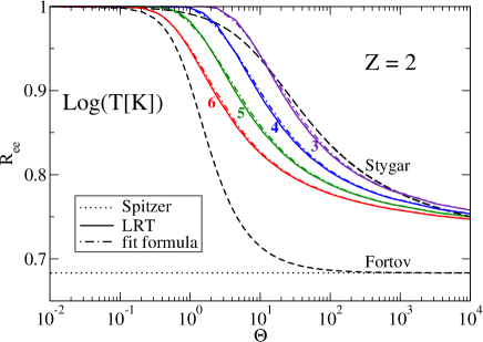
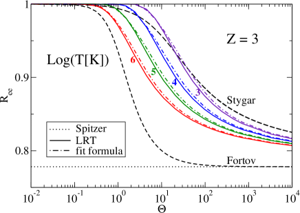
Figure 3: (Color online) Correction factor $R_{\rm ee}$ of the conductivity due to $e-e$ collisions as function of the degeneracy parameter $\Theta$ for $Z=2$ (left panel) and $Z=3$ (right panel) for different temperatures $T=(10^{3},10^{4},10^{5},10^{6})$ K; same notation as in Fig. 1.

Fig. 1 shows the results for $Z=1$ in dependence on the density and temperature. The $e-e$ interaction generally leads to a reduction of the static conductivity which is expected due to an additional scattering process. Also, this becomes less relevant with increasing degeneracy due to the Pauli exclusion effect. Fig. 3 in App. C illustrates the results for $Z=2$ and $3$, respectively. With increasing effective charge, the $e-e$ correction factor becomes smaller.

Beside the comparison of the fit formula (34) with the numerical results, Figs. 1 and 3 show the low-density limit given by Spitzer, see Eq. (29), which would be reached at very large values of $\Theta$ only. Also shown are approximations proposed by Stygar et al. stygar02

$$R_{\rm ee}^{\rm Stygar}(\Theta,Z)=R_{\rm ee}^{\rm KT}(Z)+\frac{1-R_{\rm ee}^{\rm KT}(Z)}{1+0.6\ln\left(1+\frac{\Theta}{20}\right)},$$ (41)

and Fortov et al. Fortov03

$$R_{\rm ee}^{\rm Fortov}(\Theta,Z)=R_{\rm ee}^{\rm KT}(Z)+\frac{1-R_{\rm ee}^{\rm KT}(Z)}{\sqrt{1+\Theta^{2}}},$$ (42)

with the Spitzer values $R_{\rm ee}^{\rm KT}(Z=1)=0.582$, see Eq. (29), and $R_{\rm ee}^{\rm KT}(Z=2)=0.683$, see Spitzer53 . The value $R_{\rm ee}^{\rm KT}(Z=3)=0.778$ follows from the low-density limit $1-A(Z)$ in Eq. (34). The phenomenologically constructed approximations of Fortov et al. and Stygar et al. do not include an explicit dependence on $T$. The Stygar et al. expression gives the behavior in the low-density limit qualitatively correct, whereas the behavior in the region of strong degeneracy is better described by that of Fortov et al. Fortov03 . A numerical analysis of the correction factor using gLRT has already been presented by Adams et al. in Ref. Adams07 but no fit formula was given.

The inclusion of further effects such as dynamical screening, ion-ion structure factor, and strong collisions (see Refs. RR89 ; RRMK89 ; Redmer97 ; Reinholz05 ; Karachtanov13 ) requires more detailed investigations. However, these effects are of less relevance for the correction due to $e-e$ collisions, both in the high-density and low-density limit. In the latter case, corrections appear only in higher orders of the virial expansion. Dynamical screening can be taken into account approximatively by an effective screening radius, see Refs. Karachtanov11 ; Karachtanov13 , but affects the correction factor by less than 2%.

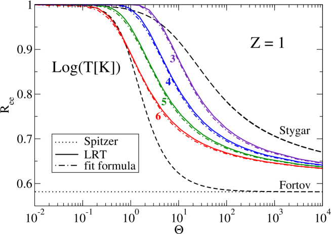
Figure 1: (Color online) Correction factor $R_{\rm ee}$ of the conductivity due to $e-e$ collisions as function of degeneracy parameter $\Theta$ at $Z=1$ for different temperatures $T=(10^{3},10^{4},10^{5},10^{6})$ K. Numerical calculations (LRT, full lines) are compared with the fit formula (34) (dot-dashed lines) and the approximations (41) of Stygar et al. stygar02 and (42) of Fortov et al. Fortov03 (dashed lines).

IV.2 The contribution of $e-e$ collisions

The discussion on the inclusion of $e-e$ collisions in the case of DFT simulations is still ongoing. However, this is crucial when comparing different approximations as will be seen in the following Subsection. Here we want to respond to an argumentation given by Dharma-wardana in Ref. dharma06 . Using the relaxation time approach, the single-center T-matrix combined with a total ion-ion structure factor derived from quantum HNC was calculated. Comparison with data for aluminum and gold show good coincidence in the region of a degenerate electron system. Here, Fermi’s golden rule and the relaxation time ansatz are justified which follows from our discussion as well.

A more general discussion in Ref. dharma06 on the role of $e-e$ interaction for the electrical conductivity argues that no resistivity can be observed because the total current is conserved under $e-e$ interaction. This seems trivial. However, it is not stringent to conclude that this is also the case in the general case of a two-component plasma. There is an indirect influence via the screening of the electron-ion pseudo-potential interaction that arises within a mean-field treatment. Even more, those collisions are entropy producing. The umklapp processes in crystalline solids ChrisRoep85 are not relevant in a plasma since there is no long-range order. It is correct that the interaction with the ion subsystem is necessary to obtain any change in the total electron current, but it cannot be said that $e-e$ interactions play no part in the static or dynamic conductivity at all.

The Spitzer result takes into account the contribution of $e-e$ collisions to the conductivity. This is due to the flexibility of the single-momentum distribution $f(\bf p)$ that is sensitive to the contribution of $e-e$ collisions. The same is also obtained introducing moments of the distribution function as done in the variational approach Redmer97 ; Reinholz05 . It is claimed and generally accepted that the Spitzer result is the benchmark for the low-density limit of a classical plasma. In contrast, the conclusion drawn in dharma06 , that this does not establish the validity of results of the Spitzer type, is not convincingly justified. The other main argument is, that good agreement between experimental data and calculations neglecting $e-e$ contributions shows that the direct role of $e-e$ interactions, taken for granted in the plasma literature, needs to be seriously reconsidered. We have shown that it is the particular case of highly degenerate WDM states where the contribution of $e-e$ collisions to the conductivity becomes small indeed. This can readily be seen from the correction factor $R_{\rm ee}(\Theta)$ that approaches the value $1$ for $\Theta\ll 1$.

IV.3 Conductivity of aluminum plasma

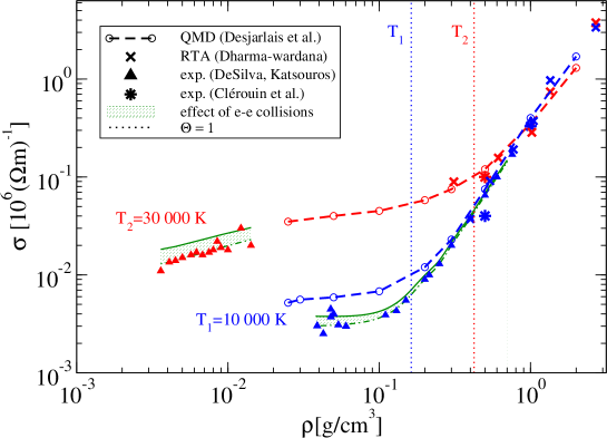
Figure 2: (Color online) Aluminum dc conductivity as function of density for 10 000 K (blue) and 30 000 K (red). Experiments were performed by DeSilva and Katsouros Silva (triangles) and Clerouin et al. Clerouin (stars) for which regression curves are given by dashed-dotted lines (green). The DFT-MD results of Desjarlais et al. Desjarlais02 are shown as hollow circles on dashed lines. Calculations of Dharma-wardana dharma06 based on the relaxation time approximation (RTA) are given as crosses. Degeneracy effects become important right to the vertical dotted lines ($\Theta=1$). Solid lines (green) show the conductivity of a hypothetical Lorentz plasma, obtained by extracting the $e-i$ scattering contributions from the regression curve (dashed-dotted line) according to the correction factor $R_{\rm ee}$, Eq. (34), for the given densities and temperatures.

The static electrical conductivity of Al plasma has been investigated experimentally by a number of groups, see e.g. Silva ; Clerouin ; Krisch98 , and also been discussed in the context of theoretical approaches, see Kuhlbrodt et al. Redmer99 ; Kuhlbrodt00 ; Kuhlbrodt01 and references there in, and Refs. dharma06 ; Desjarlais02 ; Mazevet05 ; Clerouin . Exemplarily, we consider experimental data that were theoretically analyzed by Desjarlais et al.  Desjarlais02 , see also Mazevet05 , using the Kubo-Greenwood formula (31). The results for the dc conductivity are shown in Fig. 2. The dotted lines indicate the density for which $\Theta=1$, i.e. degeneracy effects are important to the right of these lines.

For solid state densities, the electron system is degenerate ($\Theta<1$, region right to the dotted lines) and the correction factor is $R_{\rm ee}\approx 1$ there, see Figs. 1 and 3. The conductivity is essentially determined by the $e-i$ interaction whereas the $e-e$ interaction does not give a direct contribution but influences the $e-i$ pseudo-potential due to screening and exchange interactions. In this region, excellent agreement between the measured data Silva ; Clerouin and the DFT-MD simulations using the Kubo-Greenwood approach Desjarlais02 can be stated. Evaluations based on gLRT yield also the correct qualitative behavior in this region but depend on the choice for the screening function and the ion-ion structure factor Redmer99 ; Kuhlbrodt00 ; Kuhlbrodt01 , see Eq. (28).

At low densities, the aluminum plasma is at conditions where $\Theta>1$ so that the plasma is no longer degenerate. In this region, the correction factor is $R_{\rm ee}<1$, see Figs. 1 and 3, so that $e-e$ collisions contribute to the conductivity. In order to illustrate the influence of $e-e$ collisions, we propose the following procedure. Dividing the measured values by the correction factor $R_{\rm ee}$, Eq. (34), yields the contribution of the $e-i$ collisions to the conductivity, thus giving simultaneously an estimate for the effect of $e-e$ collisions. To apply the correction factor the charge state $Z$ has to be specified. We use the ionization degree calculated from coupled mass action laws, see Refs. [55, 58]. For the temperature of 30 000 K, at the densities considered here a value $Z\approx 1$ has been given. It was also found that at 10 000 K the ionization degree is much lower in this low-density region. The calculated average charge state of $Z\approx 0.1$ indicates that at most 1/10 of the Al atoms are ionized, and correspondingly the free electron density $n_{\rm e}=n_{\rm ion}\approx n_{\rm atom}/10$ is also reduced. Besides the reduced number of charge carriers, an additional scattering contribution on the neutral atoms leads to a further reduction of the the electrical conductivity as was shown in Refs. Redmer99 ; Kuhlbrodt00 ; Kuhlbrodt01 . Within a partially ionized system this may become the stronger effect than that of $e-e$ collisions. This might well justify taking the $e-e$ contribution into account via the correction factor instead of an explicit numerical calculation.

Please note that the electrical conductivity in this partially ionized, non-degenerate region $\Theta>0$ and $\Gamma<1$ strongly depends on the ionization degree of the plasma and the effective interaction between the electrons, ions, and neutral atoms. The calculation of corresponding mass action laws and two-particle potentials is the main problem in this region which has been addressed in chemical models, see Redmer99 ; Kuhlbrodt00 ; Kuhlbrodt01 . Applying DFT-MD simulations in this low-density region is a challenge since most of the DFT codes are based on plane-wave expansions which become computationally expensive there. Furthermore, the XC functional has to be chosen such that the correct band-gap (ionization energy) is reproduced. Standard XC functionals, such as given by Perdew et al. PBE , underestimate the band gap systematically MPD-CPP so that, e.g., hybrid functionals HSE have to be applied. These issues are subject of future work.

V Conclusions

We conclude that $e-e$ collisions have to be included in the low-density, nondegenerate region of WDM. Compared with calculations of the dc conductivity that take into account only $e-i$ collisions, such as the use of the relaxation time ansatz, the contribution of the $e-e$ collisions can be represented by a correction factor $R_{\rm ee}$ that depends mainly on the degeneracy parameter $\Theta$. In the case of a strongly degenerate electron gas ($\Theta\ll 1$), the contribution of $e-e$ collisions can be neglected since only umklapp processes are of relevance in solids. In the non-degenerate limit $\Theta\gg 1$, the $e-e$ collisions lead to a reduction of the dc conductivity by a factor of about 0.5 for $Z=1$. With increasing $Z$ the reduction becomes less relevant leading to the Lorentz plasma result for $Z\gg 1$.

The generalized linear response theory allows to evaluate the transport coefficients of WDM in a wide region, joining the limits of strong degeneracy known from liquid metals and of low densities as known from standard plasma physics. The present work considers free electrons interacting with ions having an effective charge $Z$. The fit formula given in Sec. IV.1 to calculate the influence of $e-e$ collisions on the conductivity allow for a better implementation in codes and other applications.

Future work will be concerned with the frequency dependence of the correction factor $R_{\rm ee}$. While it was already shown numerically in Reinholz12 , that the renormalization function is not relevant in the high frequency limit, $\lim_{(\omega_{\textrm{pl}}/\omega)\rightarrow 0}r(\omega)=1$, the intermediate frequency region has to be investigated for any degeneracy.

The implementation of pseudo-potentials and the ion-ion structure factor become of relevance with increasing free electron density. However, at high densities, the influence of the renormalization function is fading, $r(\omega)\to 1$. Therefore these effects are of high relevance for the $e-i$ collisions determining the collision frequency $\nu^{\textrm{Ziman}}$, but barely relevant for the correction factor $R_{\rm ee}$.

Another issue is the composition of WDM in the low-density, low-temperature limit where a chemical model is applicable. The ionization degree and composition are derived from a mass action law, that gives the effective charge $Z$ in dependence of temperature $T$ and ion density $n_{\rm ion}$. In particular, for the partially ionized plasma, additional scattering with neutrals will reduce the conductivity at low temperatures considerably. Further work is necessary in order to relate predictions of chemical models to those based on DFT, and to clarify the role of $e-e$ collisions within DFT-MD in the low-density limit.

Appendix A Generalized linear response theory

In the case of a charged particle system considered here, described by the Hamiltonian $\hat{H}$, under the influence of an external field, $\hat{H}_{F}(t)=-e{\bf\hat{r}}{\bf E}^{\rm ext}(t)$, the non-equilibrium statistical operator has to be determined. Following Zubarev ZMR1 ; Roep98 ; Reinholz05 ; Reinholz00 , one starts with a relevant statistical operator

$$\hat{\rho}_{\rm rel}(t)=\frac{1}{Z_{\rm rel}(t)}\textrm{e}^{-\beta(\hat{H}-\mu\hat{N})+\sum_{l}F_{l}(t)\hat{B}_{l}},\qquad Z_{\rm rel}(t)=\textrm{Tr}\left\{{\textrm{e}^{-\beta(\hat{H}-\mu\hat{N})+\sum_{l}F_{l}(t)\hat{B}_{l}}}\right\}\,,$$ (43)

as a generalized Gibbs ensemble which is derived from the principle of maximum of the entropy. This relevant distribution is characterized by a set of relevant observables $\{\hat{B}_{l}\}$ chosen in addition to energy $\hat{H}$ and number of particles $\hat{N}$. The Lagrange parameters $\beta,\mu,F_{l}(t)$, which are real valued numbers, are introduced to fix the given averages

$$\textrm{Tr}\left\{{\hat{B}_{l}\,\hat{\rho}(t)}\right\}=\langle\hat{B}_{l}\rangle^{t}=\textrm{Tr}\left\{{\hat{B}_{l}\,\hat{\rho}_{\rm rel}(t)}\right\}\,.$$ (44)

These self-consistent conditions ensures that the observed averages $\langle\hat{B}_{l}\rangle^{t}$ are exactly reproduced by the hermitian $\hat{\rho}_{\rm rel}(t)$. Similar relations are used in equilibrium to eliminate the Lagrange parameters $\beta$ and $\mu$. Starting with the relevant statistical operator, the stationary non-equilibrium state is formed dynamically, and this process converges the faster the more relevant observables $\hat{B}_{l}$ are included to characterize the initial state. The selection of the set of relevant observables has no influence on the result if the calculations are performed rigorously, but will influence the result if approximations such as perturbation expansions are performed.

In linear response, the response parameters $F_{l}(t)$ are considered to be small so that we can solve the implicit relation (44). The response parameter are determined after expanding up to the first order with respect to the external field ${\bf E}^{\text{ext}}(\omega)$ (we consider a homogeneous field, e.g. zero wave vector) and the response parameters $F_{l}$, where $F_{l}(t)={\rm Re}\{F_{l}\textrm{e}^{-i\omega t}\}$. We arrive at the response equations Reinholz12

$$\sum_{l^{\prime}}\left[\left({\hat{B}}_{l};\dot{\hat{B}}_{l^{\prime}}\right)+\left<\dot{\hat{B}}_{l};\dot{\hat{B}}_{l^{\prime}}\right>_{z}-i\omega\left\{\left({\hat{B}}_{l};{\hat{B}}_{l^{\prime}}\right)+\left<\dot{\hat{B}}_{l};\delta{\hat{B}}_{l^{\prime}}\right>_{z}\right\}\right]F_{l^{\prime}}=\beta\frac{e}{m}\left\{\left({\hat{B}}_{l};{\bf\hat{P}}\right)+\left<\dot{\hat{B}}_{l};{\bf\hat{P}}\right>_{z}\right\}\cdot{\bf E}^{\text{ext}}(\omega)\,$$ (45)

with $z=\omega+i\eta$ ($\lim_{\eta\to+0}$) and the Laplace transform of the correlation functions, Eq. (4). The time derivative of the position operator in $\hat{H}_{F}(t)$ leads to the total momentum ${\bf\hat{P}}=\sum_{p}{\bf p}\,\hat{n}_{p}$, and subsequently to the right hand side of Eq. (45).

Considering $L$ relevant observables $\delta\hat{B}_{l}=\hat{B}_{l}-{\rm Tr}\{\hat{B}_{l}\rho_{0}\}$, Eq. (45) is a system of $L$ linear equations to determine the response parameters $F_{l}$ for a given external field ${\bf E}^{\text{ext}}(\omega)$. It is the most general form of LRT, allowing for arbitrary choice of relevant observables $\hat{B}_{l}$ and corresponding response parameters $F_{l}$. Comparing with kinetic theory Reinholz12 , the first correlation function on the left hand side can be identified as a collision term, while the right hand side represents the drift term due to the external perturbing field.

The set of relevant observables $\hat{B}_{l}$ to characterize the non-equilibrium state can be chosen arbitrarily, and the calculated non-equilibrium properties are independent on this choice provided no approximations like perturbation expansions are performed. At least, the set of relevant observables $\hat{B}_{l}$ should contain conserved quantities that determine the equilibrium state. Conveniently, also long-living fluctuations in the system that are hardly produced by the dynamical evolution (such as bound state formation) should be taken into account. Otherwise, a perturbation expansion is converging only slowly. Different expressions and results can be understood as approximations, working in a Markov approximation and describing the system on different levels of sophistication. Results that are obtained in lowest order are improved summing up (sometimes divergent) terms that occur in higher order perturbative expansions. Alternatively, we can suggest different choices of the set of relevant observables $\hat{B}_{l}$ like a variational approach (Kohler variational principle), see Reinholz12 .

Starting with the occupation numbers $\hat{n}_{p}$ of the single-particle states $|p\rangle$ as set of relevant observables $\hat{B}_{l}$, we arrive at the generalized linear Boltzmann equations Reinholz12 ($\delta\dot{\hat{n}}_{p}=\dot{\hat{n}}_{p}$)

$$\sum_{p^{\prime}}\left[(\delta\hat{n}_{p},\dot{\hat{n}}_{p^{\prime}})+\left<\dot{\hat{n}}_{p};\dot{\hat{n}}_{p^{\prime}}\right>_{z}-i\omega\left\{(\delta{\hat{n}}_{p},\delta\hat{n}_{p^{\prime}})+\left<\dot{\hat{n}}_{p};\delta{\hat{n}}_{p^{\prime}}\right>_{z}\right\}\right]F_{p^{\prime}}=\frac{e}{m}\beta\sum_{p^{\prime\prime}}\left[(\delta\hat{n}_{p},{\hat{n}}_{p^{\prime\prime}})+\left<\dot{\hat{n}}_{p};{\hat{n}}_{p^{\prime\prime}}\right>_{z}\right]{\bf p}^{\prime\prime}\cdot{\bf E}^{\text{ext}}(\omega)\,.$$ (46)

This is the basic equation to work out the linear response approach given in Sec. II.1.

Appendix B Calculation and simplification of the correlation functions, Eqs. (III.1, III.1)

The expression (III.1),

$$d_{ll^{\prime}}^{\rm ei} = \pi\hbar Z^{2}2(2s_{i}+1)\sum_{\bf{k}\bf{p}\bf{q}}\int\limits_{-\infty}^{\infty}d\hbar\omega\left|\frac{V(q)}{\epsilon^{\rm RPA}(q,\omega)}\right|^{2}f_{k}^{e}(1-f_{\left|\bf{k}+\bf{q}\right|}^{e})f_{p}^{i}(1-f_{\left|\bf{p}-\bf{q}\right|}^{i})$$ (47)

$$\times\delta(\hbar\omega-E_{\left|\bf{k}+\bf{q}\right|}^{e}+E_{k}^{e})\delta(\hbar\omega-E_{p}^{i}+E_{\left|\bf{p}-\bf{q}\right|}^{i})K_{l}({\bf k},{\bf q})K_{l^{\prime}}({\bf k},{\bf q})\,,$$

is evaluated by performing the integral over $\hbar\omega$. In the resulting $\delta$ function that describes energy conservation, we can neglect the ionic contributions because of the large mass ratio (adiabatic limit, elastic collisions of the electrons at the fixed ions). The ions are treated classically, and the summation over $\bf p$ and spin summation gives simply $(2s_{i}+1)\sum_{\bf p}f^{i}_{p}=n_{\rm ion}\Omega=N_{\rm ion}$, the number of ions. In particular,

$$d_{11}^{\rm ei} = 2\pi\hbar Z^{2}n_{\rm ion}\Omega\sum_{\bf{k}\bf{q}}\left[\frac{e^{2}}{\epsilon_{0}\Omega(q^{2}+\kappa^{2})}\right]^{2}f_{k}^{e}(1-f_{\left|\bf{k}+\bf{q}\right|}^{e})\delta(E_{k}^{e}-E_{\left|\bf{k}+\bf{q}\right|}^{e})q_{z}^{2}\,,$$ (48)

or with $q_{z}^{2}\to q^{2}/3$ and transforming the $\delta$ function

$$d_{11}^{\rm ei} = \frac{e^{4}}{(4\pi\epsilon_{0})^{2}}\frac{32\pi^{2}}{3}\pi\hbar Z^{2}n_{\rm ion}\Omega\frac{4\pi\,2\pi}{(2\pi)^{6}}\int_{0}^{\infty}dq\frac{q^{4}}{(q^{2}+\kappa^{2})^{2}}\int_{0}^{\infty}dk\,k^{2}\,f_{k}^{e}(1-f_{k}^{e})\int_{-1}^{1}dz\,\delta\left(z+\frac{q}{2k}\right)\frac{m}{\hbar^{2}kq}\,.$$ (49)

Now, the integral over $z$ can be performed so that $k\leq q/2$, and we transform the $k$ integral as $k\,dk=dk^{2}/2=d(\beta E_{k})m/(\hbar^{2}\beta)$ (note that the superscript $e$ for electrons is omitted throughout the rest of this appendix),

$$d_{11}^{\rm ei} = \frac{e^{4}}{(4\pi\epsilon_{0})^{2}}\frac{4}{3\pi^{2}}\pi\hbar Z^{2}n_{\rm ion}\Omega\frac{m}{\hbar^{2}}\int_{0}^{\infty}dq\frac{q^{3}}{(q^{2}+\kappa^{2})^{2}}\left(-\frac{m}{\hbar^{2}\beta}\right)\int_{\beta\hbar^{2}q^{2}/(8m)}^{\infty}d(\beta E_{k})\frac{d}{d(\beta E_{k})}\frac{1}{e^{\beta E_{k}-\beta\mu_{e}^{\rm id}}+1}\,,$$ (50)

so that the integral over $k$ is performed,

$$d_{11}^{\rm ei} = \frac{e^{4}}{(4\pi\epsilon_{0})^{2}}\frac{4}{3\pi^{2}}\pi\hbar Z^{2}n_{\rm ion}\Omega\frac{m^{2}}{\hbar^{4}\beta}\int_{0}^{\infty}dq\frac{q^{3}}{(q^{2}+\kappa^{2})^{2}}\frac{1}{e^{\beta\hbar^{2}q^{2}/(8m)-\beta\mu_{e}^{\rm id}}+1}$$ (51)

or, using dimensionless $Q=\sqrt{\beta\hbar^{2}q^{2}/m}$,

$$d_{11}^{\rm ei} = Zd\frac{2}{n_{\rm e}\Lambda_{e}^{3}}\int_{0}^{\infty}dQ\;\frac{Q^{3}}{(Q^{2}+\frac{\hbar^{2}\beta}{m}\kappa^{2})^{2}}\;\frac{1}{e^{Q^{2}/8-\alpha}+1}\,,$$ (52)

with $\alpha=\beta\mu_{e}^{\rm id}$, the thermal wavelength $\Lambda_{e}$ (see below Eq. (III.1) in Sec. III.1) and the prefactor

$$d=\frac{4}{3}(2\pi)^{1/2}Z^{2}n_{\rm ion}^{2}\Omega m^{1/2}\beta^{1/2}\frac{e^{4}}{(4\pi\epsilon_{0})^{2}}.$$ (53)

In analogy to Eq. (52) we now calculate the correlation functions (47) with higher moments. With $K_{1}({\bf k},{\bf q})=-q_{z},\,\,\,K_{3}({\bf k},{\bf q})=-q_{z}(\beta E_{k})$, and replacing $(\beta E_{k})\to x$ we find

$$d_{ll^{\prime}}^{\rm ei} = Zd\frac{2}{n_{\rm e}\Lambda_{e}^{3}}\int_{0}^{\infty}dQ\frac{Q^{3}}{(Q^{2}+\frac{\hbar^{2}\beta}{m}\kappa^{2})^{2}}S_{ll^{\prime}}(Q),$$ (54)

with

$$S_{11}(Q)=\frac{1}{e^{Q^{2}/8-\alpha}+1},$$

$$S_{13}(Q)=S_{31}(Q)=\frac{Q^{2}/8}{e^{Q^{2}/8-\alpha}+1}+\int_{Q^{2}/8}^{\infty}dx\frac{1}{e^{x-\alpha}+1},$$

$$S_{33}(Q)=\frac{Q^{4}/64}{e^{Q^{2}/8-\alpha}+1}+2\int_{Q^{2}/8}^{\infty}dx\frac{x}{e^{x-\alpha}+1}.$$

We evaluate the $e-e$ correlation functions, Eq. (III.1), in the lowest non-vanishing order. Because of total momentum conservation, $d_{11}^{\rm ee}=d_{13}^{\rm ee}=0$. The first and only correlation function within two-moment approach is

$$d_{33}^{\rm ee}=2\pi\beta^{2}\hbar\sum_{\bf{k}\bf{p}\bf{q}}\int\limits_{-\infty}^{\infty}d\hbar\omega\left|\frac{V(q)}{\epsilon^{\rm RPA}(q,\omega)}\right|^{2}f(E_{k})(1-f(E_{k}+\hbar\omega))f(E_{p})(1-f(E_{p}-\hbar\omega))$$ (55)

$$\times\delta(\hbar\omega-E_{\left|\bf{k}+\bf{q}\right|}+E_{k})\delta(\hbar\omega-E_{p}+E_{\left|\bf{p}-\bf{q}\right|})\left[k_{z}E_{k}-(k_{z}+q_{z})(E_{k}+\hbar\omega)+p_{z}E_{p}-(p_{z}-q_{z})(E_{p}-\hbar\omega)\right]^{2}.$$

The dynamically screened Coulomb potential will be replaced by the static Debye potential, see Sec. III.1. The effect of dynamical screening that leads to the Lenard-Balescu expression for the conductivity has been discussed elsewhere Redmer97 . For the evaluation, using spherical coordinates, we obtain

$$d_{33}^{\rm ee} = \beta^{2}\hbar\frac{2\pi\Omega^{3}}{3(2\pi)^{9}}\int d^{3}q\int\limits_{-\infty}^{\infty}d\hbar\omega\int d^{3}p\int d^{3}k\left|\frac{e^{2}}{\epsilon_{0}\Omega(q^{2}+\kappa^{2})}\right|^{2}f(E_{k})(1-f(E_{k}+\hbar\omega))f(E_{p})(1-f(E_{p}-\hbar\omega))$$ (56)

$$\times\delta\left(\hbar\omega-\frac{\hbar^{2}kq\cos\theta_{k}}{m}-\frac{\hbar^{2}q^{2}}{2m}\right)\delta(\hbar\omega-\frac{\hbar^{2}pq\cos\theta_{p}}{m}+\frac{\hbar^{2}q^{2}}{2m})$$

$$\times\left[q^{2}(E_{p}-E_{k})^{2}+2{\bf q}\cdot({\bf p}-{\bf k}-2{\bf q})(E_{p}-E_{k})\hbar\omega+({\bf p}-{\bf k}-2{\bf q})^{2}\hbar^{2}\omega^{2}\right].$$

The angles between the $q$-direction and the direction of $k$ or $p$ are denoted by $\theta_{k}$ and $\theta_{p}$, respectively.

The square brackets written in spherical coordinates are

$$\left[\frac{\hbar^{4}}{4m^{2}}q^{2}(p^{2}-k^{2})^{2}+\frac{\hbar^{2}}{m}(pq\cos\theta_{p}-qk\cos\theta_{k}-2q^{2})(p^{2}-k^{2})\hbar\omega\right.$$ (57)

$$\left.+(p^{2}+k^{2}+4q^{2}-4pq\cos\theta_{p}+4kq\cos\theta_{k}-2pk(\cos\theta_{p}\cos\theta_{k}+\sin\theta_{p}\sin\theta_{k}(\cos\phi_{p}\cos\phi_{k}+\sin\phi_{p}\sin\phi_{k}))\hbar^{2}\omega^{2}\right].$$

The last parentheses can be rewritten as $\cos\phi_{p}\cos\phi_{k}+\sin\phi_{p}\sin\phi_{k}=\cos(\phi_{p}-\phi_{k})$. $\phi_{p}-\phi_{k}$ can be introduced as new variable, the integral vanishes. We are left with

$$d_{33}^{\rm ee}=\beta^{2}\hbar\frac{4\pi\Omega}{3(2\pi)^{6}}\frac{m^{2}}{\hbar^{4}}\int_{0}^{\infty}dq\,q^{2}\int\limits_{-\infty}^{\infty}d\hbar\omega\int_{0}^{\infty}dk\,k^{2}\int_{-1}^{1}dz_{k}\int_{0}^{\infty}dp\,p^{2}\int_{-1}^{1}dz_{p}\,\frac{e^{4}}{(q^{2}+\kappa^{2})^{2}}$$

$$\times f(E_{k})(1-f(E_{k}+\hbar\omega))f(E_{p})(1-f(E_{p}-\hbar\omega))\frac{1}{kq}\delta\left(z_{k}+\frac{q}{2k}-\frac{m\omega}{\hbar kq}\right)\frac{1}{pq}\delta\left(z_{p}-\frac{q}{2p}-\frac{m\omega}{\hbar pq}\right)$$

$$\times\left[q^{2}\frac{\hbar^{4}}{4m^{2}}(p^{2}-k^{2})^{2}+2(qpz_{p}-qkz_{k}-2q^{2})\frac{\hbar^{2}}{2m}(p^{2}-k^{2})\hbar\omega+(p^{2}+k^{2}+4q^{2}-4pqz_{p}+4kqz_{k}-2pkz_{p}z_{k})\hbar^{2}\omega^{2}\right].$$

Introducing dimensionless variables $Q$ as defined above and $x=\sqrt{\beta E_{k}},\;y=\sqrt{\beta E_{p}},\;\omega=\nu Q/(\beta\hbar)$, and performing the integrals over $z_{p},z_{k}$, we have

$$d_{33}^{\rm ee} = \frac{16\pi e^{4}\Omega m^{7/2}}{3\epsilon_{0}^{2}(2\pi)^{6}\beta^{5/2}\hbar^{6}}\int_{0}^{\infty}dQ\,\frac{Q^{3}}{(Q^{2}+\frac{\hbar^{2}\beta}{m}\kappa^{2})^{2}}\int\limits_{-\infty}^{\infty}d\nu\int_{|\nu-Q/2|/\sqrt{2}}^{\infty}dx\,x\int_{|\nu+Q/2|/\sqrt{2}}^{\infty}dy\,y$$

$$\times\frac{1}{e^{x^{2}-\alpha}+1}\frac{1}{1+e^{-x^{2}-\nu Q+\alpha}}\frac{1}{e^{y^{2}-\alpha}+1}\frac{1}{1+e^{-y^{2}+\nu Q+\alpha}}$$

$$\times\left[(y^{2}-x^{2})^{2}-2(y^{2}-x^{2})\nu Q+2(y^{2}+x^{2})\nu^{2}-4\left(\frac{\nu^{2}}{2}-\frac{Q^{2}}{8}\right)\nu^{2}\right].$$

Now we substitute $x^{2}=\hat{x}+\nu^{2}/2-\nu Q/2+Q^{2}/8,\,\,\,y^{2}=\hat{y}+\nu^{2}/2+\nu Q/2+Q^{2}/8$, thus shifting the lower bound of the $x$ and $y$ integral to zero. In general the final expression

$$d_{33}^{\rm ee} =\frac{d}{\sqrt{2\pi}}\frac{2}{n_{\rm e}^{2}\Lambda_{e}^{6}}\int_{0}^{\infty}dQ\frac{Q^{3}}{\left(Q^{2}+\frac{\hbar^{2}\beta}{m}\kappa^{2}\right)^{2}}f_{33}^{\rm ee}(\alpha,Q)\qquad\textrm{with}$$

$$f_{33}^{\rm ee}(\alpha,Q) =\int\limits_{-\infty}^{\infty}d\nu\int_{0}^{\infty}d{\hat{x}}\int_{0}^{\infty}d{\hat{y}}\left[({\hat{y}}-{\hat{x}})^{2}+2\nu^{2}({\hat{y}}+{\hat{x}})\right]\frac{1}{e^{{\hat{x}}+\nu^{2}/2-\nu Q/2+Q^{2}/8-\alpha}+1}$$

$$\times\frac{1}{1+e^{-{\hat{x}}-\nu^{2}/2-\nu Q/2+\alpha-Q^{2}/8}}\frac{1}{e^{{\hat{y}}+\nu^{2}/2+\nu Q/2+Q^{2}/8-\alpha}+1}\frac{1}{1+e^{-{\hat{y}}-\nu^{2}/2+\nu Q/2+\alpha-Q^{2}/8}},$$

is evaluated numerically. For the classical limit an analytical expression can be given, see App. C.

Appendix C Correlation functions in the classical limit and construction of a fit formula

Expressions for the correlation functions derived in App. B are further analyzed in the limit of non-degeneracy. We introduce integrals of the form:

$$J_{1,b} =\int\limits_{0}^{\infty}dQ\frac{Q^{3}}{(Q^{2}+\frac{\hbar^{2}\beta}{m}\kappa^{2})^{2}}\frac{1}{e^{Q^{2}/8-\alpha}+1}\left(\frac{Q^{2}}{8}\right)^{b},$$ (61)

$$J_{2,b} =\int\limits_{0}^{\infty}dQ\frac{Q^{3}}{(Q^{2}+\frac{\hbar^{2}\beta}{m}\kappa^{2})^{2}}\int\limits_{0}^{\infty}dx\frac{(x+Q^{2}/8)^{b}}{e^{x+Q^{2}/8-\alpha}+1},$$ (62)

$$J_{3} =\int\limits_{0}^{\infty}dQ\frac{Q^{3}}{(Q^{2}+\frac{\hbar^{2}\beta}{m}\kappa^{2})^{2}}f_{33}^{\rm ee}(\alpha,Q),$$ (63)

For the correlation functions, Eqs. (54, B), we find:

$$\frac{d_{11}}{\Omega} =Zd\frac{2}{n_{\rm e}\Lambda_{e}^{3}}\cdot J_{1,b=0},$$ (64)

$$\frac{d_{13}}{\Omega} =Zd\frac{2}{n_{\rm e}\Lambda_{e}^{3}}\cdot\left(J_{1,b=1}+J_{2,b=0}\right),$$ (65)

$$\frac{d_{33}^{\rm ei}}{\Omega} =Zd\frac{2}{n_{\rm e}\Lambda_{e}^{3}}\cdot\left(J_{1,b=2}+2\cdot J_{2,b=1}\right),$$ (66)

$$\frac{d_{33}^{\rm ee}}{\Omega} =\frac{d}{\sqrt{2\pi}}\frac{2}{n_{\rm e}^{2}\Lambda_{e}^{6}}\cdot J_{3}.$$ (67)

In the classical limit ($\alpha<<0$, $\kappa^{2}\approx\kappa^{2}_{\rm D}=\beta(1+Z)n_{\rm e}e^{2}/\epsilon_{0}$) the integrals yield

$$J_{1,b} =e^{\alpha}\int\limits_{0}^{\infty}dQ\frac{Q^{3}}{(Q^{2}+\frac{\hbar^{2}\beta}{m}\kappa^{2})^{2}}e^{-Q^{2}/8}\left(\frac{Q^{2}}{8}\right)^{b}=e^{\alpha}\cdot\begin{cases}-\frac{1}{2}\mathrm{Ei}\left(-\tilde{k}^{2}\right)&b=0\\ \frac{1}{2}&b=1;2\end{cases},$$ (68)

$$J_{2,b=0} =e^{\alpha}\int\limits_{0}^{\infty}dQ\frac{Q^{3}}{(Q^{2}+\frac{\hbar^{2}\beta}{m}\kappa^{2})^{2}}e^{-Q^{2}/8}=J_{1,b=0},$$ (69)

$$J_{2,b=1} =e^{\alpha}\int\limits_{0}^{\infty}dQ\frac{Q^{3}}{(Q^{2}+\frac{\hbar^{2}\beta}{m}\kappa^{2})^{2}}e^{-Q^{2}/8}\left(\frac{Q^{2}}{8}+1\right)=J_{1,b=0}+J_{1,b=1},$$ (70)

$$J_{3} =e^{2\alpha}\int\limits_{0}^{\infty}dQ\frac{Q^{3}}{(Q^{2}+\frac{\hbar^{2}\beta}{m}\kappa^{2})^{2}}e^{-2Q^{2}/8}\underbrace{\int\limits_{-\infty}^{\infty}d\nu\int\limits_{0}^{\infty}d{\hat{x}}\int\limits_{0}^{\infty}d{\hat{y}}\,e^{-{\hat{x}}-{\hat{y}}-\nu^{2}}[({\hat{y}}-{\hat{x}})^{2}+2\nu^{2}({\hat{y}}+{\hat{x}})]}_{4\sqrt{\pi}}$$ (71)

$$=-4\sqrt{\pi}e^{2\alpha}\cdot\frac{1}{2}\mathrm{Ei}\left(-2\tilde{k}^{2}\right)=-4\sqrt{\pi}e^{2\alpha}\cdot\left(\frac{1}{2}\mathrm{Ei}\left(-\tilde{k}^{2}\right)+\frac{\ln(2)}{2}\right),$$ (72)

with the coefficient $\tilde{k}^{2}=\tilde{k}^{2}(\alpha)=\frac{\hbar^{2}\beta}{8m}\kappa_{\rm D}^{2}=\frac{(1+Z)\cdot e^{2}}{\pi^{2}\hbar\epsilon_{0}}e^{\alpha}\sqrt{\frac{2m}{k_{B}T}}$, the exponential integral $\mathrm{Ei}(x)=-\int\limits_{-x}^{\infty}\frac{e^{-t}}{t}dt=\gamma+\ln|x|+{\cal O}(x)$ and $\gamma$ as Euler’s constant, see Sec. III.2. The term in order of $\tilde{k}^{2}$ is neglected, we approximate $\mathrm{Ei}\left(-\tilde{k}^{2}\right)\approx\gamma+\ln\left|-\tilde{k}^{2}\right|$, and therefore $\mathrm{Ei}(-2\tilde{k}^{2})\approx\mathrm{Ei}(-\tilde{k}^{2})+\ln(2)$. We obtain for the fractions of correlation functions:

$$\frac{N_{13}}{N_{11}} =\frac{5}{2},$$ (73)

$$\frac{d_{13}}{d_{11}} =1-\frac{1}{\mathrm{Ei}(-\tilde{k}^{2})},$$ (74)

$$\frac{d_{33}^{\rm ei}}{d_{11}} =2-\frac{3}{\mathrm{Ei}(-\tilde{k}^{2})},$$ (75)

$$\frac{d_{33}^{\rm ee}}{d_{11}} =\frac{\sqrt{2}}{Z}\left(1+\frac{\ln(2)}{\mathrm{Ei}(-\tilde{k}^{2})}\right).$$ (76)

For the renormalization functions (19) in two-moment approximation in the classical case we find

$$r_{\rm ei}^{\rm cl}(\alpha) =\frac{4}{13}-\frac{84}{169}\frac{1}{{\rm Ei}(-\tilde{k}^{2})}+{\cal O}\left(\frac{1}{{\rm Ei}(-\tilde{k}^{2})}\right)^{2},$$ (77)

$$r_{\rm ei+ee}^{\rm cl}(\alpha) =\frac{4(Z+\sqrt{2})}{13Z+4\sqrt{2}}+\frac{12Z\left[\sqrt{2}\left(\ln(8)+4\right)-7Z\right]}{(13Z+4\sqrt{2})^{2}}\frac{1}{\mathrm{Ei}(-\tilde{k}^{2})}+{\cal O}\left(\frac{1}{{\rm Ei}(-\tilde{k}^{2})}\right)^{2},$$ (78)

for the Lorentz plasma and the plasma with $e-e$ correlations, respectively. The correction factor (33) is then given as

$$R_{\rm ee}^{\rm cl}(\alpha) =\frac{r_{\rm ei}(\alpha)}{r_{\rm ei+ee}(\alpha)}$$ (79)

$$=1-\frac{9\sqrt{2}}{13(\sqrt{2}+Z)}-\frac{3\left[\sqrt{2}Z\left(67+39\ln(2)\right)+56\right]}{169(Z+\sqrt{2})^{2}}\frac{1}{{\rm Ei}(-\tilde{k}^{2})}+{\cal O}\left(\frac{1}{{\rm Ei}(-\tilde{k}^{2})}\right)^{2}.$$ (80)

Instead of the degeneracy $\alpha$ the correction factor can be rewritten as a function of the degeneracy parameter $\Theta$

$$R_{\rm ee}(\Theta\gg 1) =1-A(Z)+B(Z)\left(\ln\frac{1}{C(T,Z)}\frac{3\sqrt{\pi}}{4}\Theta^{3/2}\right)^{-1},$$ (81)

because of $\alpha\approx\ln(\frac{4}{3\sqrt{\pi}}\Theta^{-3/2})$ in classical regimes. The functions $A(Z)$, $B(Z)$ and $C(T,Z)$ are given in Eqs. (35-37).

In the classical limit, the asymptotic behavior of the correction factor with respect to the temperature is given analytically with Eq. (81). In the degeneracy limit ($\alpha\gg 0$, $\Theta\ll 1$), the correlation function $d_{33}^{\rm ee}=0$, so that the correction factor $R_{\rm ee}=1$. Therefore we construct a fit-function $R_{\rm ee}$ in which the analytical classical result goes to $1$ for high degeneracy, see the first three terms of Eq. (34) in relation to Eq. (81). Eq. (34) includes a fit coefficient $a$ which doesn’t affect the classical limit and can be used for a better adjustment in the intermediate range. Finally, the discrepancy between our fit formula and numerical results was reduced by a Gaussian-like term, see the last term of Eq. (34).

The fit formula Eq. (34) for the correction factor $R_{\rm ee}$ is now compared with the numerical evaluation using the expressions for the correlation functions according to (54, B) in App. B in Figs. 1 ($Z=1$) and 3 ($Z=2,3$).

Appendix D Broadening of the $\delta$-function

Another topic is the broadening of the $\delta$-function to make a smooth transition in the static case ($\omega\to 0$ ). For the application of the Kubo-Greenwood formula given as Eq. (31), Desjarlais et al. Desjarlais02 pointed out: ”In practice, because of the finite simulation volume and resulting discrete eigenvalues, the $\delta$-function must be broadened. We use a Gaussian broadening of the $\delta$-function that is as small as feasible without recovering the local oscillations in the optical conductivity resulting from the discrete band structure”.

To discuss expression (31), we consider a finite value for $\eta$,

$$\delta_{\eta}(z)=\frac{\eta}{\eta^{2}+z^{2}}.$$ (82)

The finite width of the $\delta$ function can be interpreted as an additional damping to overcome the level spacing due to the finite volume with periodic boundary conditions. The limit $\eta\rightarrow 0$ can be taken only in the final expressions, summing up all orders of perturbation expansion. Expanding with respect to interaction $\hat{V}$, the van Hove limit ($\hat{V}^{2}/\eta\to 0$) has to be taken, see HC75 . Therefore, for finite $\eta$ a perturbation expansion of (31) can be performed.

With the perturbation expansion

$$\langle k_{1}|{\bf\hat{p}}|k_{2}\rangle=\hbar{\bf k}_{1}\delta_{k_{1},k_{2}}+\frac{\langle k_{1}|\hat{V}|k_{2}\rangle}{E_{1}-E_{2}}(\hbar{\bf k}_{1}-\hbar{\bf k}_{2})$$ (83)

we have with ${\bf k}_{2}={\bf k}_{1}+{\bf q}$ and $\langle k_{1}|\hat{V}|k_{2}\rangle=V_{q}$

$${\rm Re}\,\sigma^{\rm KG}(0)=\frac{\pi e^{2}\hbar}{3m^{2}\Omega}\sum_{k,q}\frac{\partial f(E_{k})}{\partial E_{k}}\left({\bf k}\delta_{q,0}+\frac{V_{q}}{E_{k}-E_{k+q}}{\bf q}+\dots\right)^{2}\frac{\eta}{\eta^{2}+(E_{k}-E_{k+q})^{2}}.$$ (84)

Considering the screened interaction with uncorrelated ions in the nondegenerate case, $V_{q}^{2}=N_{\rm ion}Z^{2}e^{4}/[\epsilon_{0}\Omega(q^{2}+\kappa^{2})]^{2}$, Eq. (84) leads to

$${\rm Re}\,\sigma^{\rm KG}(0)=\frac{\pi e^{2}\hbar\beta}{3m^{2}}\int\frac{d^{3}k}{(2\pi)^{3}}f(E_{k})\left(k^{2}\frac{1}{\eta}+\int\frac{d^{3}q}{(2\pi)^{3}}\frac{n_{\rm ion}Z^{2}e^{4}}{[\epsilon_{0}(q^{2}+\kappa^{2})]^{2}(E_{k}-E_{k+q})^{2}}q^{2}\frac{\eta}{\eta^{2}+(E_{k}-E_{k+q})^{2}}+\dots\right).$$ (85)

Before the last term is reinterpreted as a $\delta$-function, we estimate the denominator $E_{k}-E_{k+q}$ by the broadening parameter $\eta$ of the $\delta_{\eta}$ function so that

$${\rm Re}\,\sigma^{\rm KG}(0)=\frac{\pi e^{2}\hbar\beta}{3m^{2}}\int\frac{d^{3}k}{(2\pi)^{3}}f(E_{k})k^{2}\tau^{\rm KG}(k)+\dots$$ (86)

with

$$\tau^{\rm KG}(k) = \frac{1}{\eta}+\frac{1}{k^{2}}\int\frac{d^{3}q}{(2\pi)^{3}}\frac{n_{\rm ion}Z^{2}e^{4}}{[\epsilon_{0}(q^{2}+\kappa^{2})]^{2}(E_{k}-E_{k+q})^{2}}q^{2}\frac{\eta}{\eta^{2}+(E_{k}-E_{k+q})^{2}}+\dots$$ (87)

$$=\frac{1}{\eta}+\frac{1}{k^{2}}\frac{n_{\rm ion}Z^{2}e^{4}}{\epsilon^{2}_{0}}\int_{0}^{\infty}\frac{dq}{(2\pi)^{2}}\frac{q^{4}}{(q^{2}+\kappa^{2})^{2}}\left(\frac{m}{\hbar^{2}kq}\right)^{3}\int_{-1}^{1}dz\frac{\eta m/kq}{(\eta m/kq)^{2}+(z+q/2k)^{2}}\frac{1}{(z+q/2k)^{2}}$$

$$=\frac{1}{\eta}+\frac{1}{k^{2}}\frac{n_{\rm ion}Z^{2}e^{4}}{\epsilon^{2}_{0}}\int_{0}^{\infty}\frac{dq}{(2\pi)^{2}}\frac{q^{4}}{(q^{2}+\kappa^{2})^{2}}\left(\frac{m}{\hbar^{2}kq}\right)^{3}\left[\frac{\hbar^{2}kq}{\eta m}\frac{2}{1-(q/2k)^{2}}+\pi\left(\frac{\hbar^{2}kq}{\eta m}\right)^{2}\right]$$

$$=\frac{1}{\eta}+\frac{1}{\eta^{2}}\frac{1}{k^{3}}\frac{n_{\rm ion}Z^{2}e^{4}m\pi}{\epsilon^{2}_{0}\hbar^{2}}\int_{0}^{2k}\frac{dq}{(2\pi)^{2}}\frac{q^{3}}{(q^{2}+\kappa^{2})^{2}}+{\cal O}\left(\frac{e^{4}}{\eta}\right)\,.$$

In principle, one has to sum the leading divergent terms $\propto(1/\eta)\left(e^{4}/\eta\right)^{n}$. We give here only the first contributions,

$$\frac{1}{\eta}+\frac{1}{\eta^{2}}A+\dots=\frac{1}{\eta}\left[1+\frac{1}{\eta}A+\dots\right]=\frac{1}{\eta}\frac{1}{1-\frac{1}{\eta}A+\dots}.$$ (88)

Now the limit $\eta\to 0$ can be performed with the result $-1/A$.

For comparison, see Reinholz12 , with the golden rule for the transition rates and $S(q)\approx 1\rightarrow|V_{\textrm{ei}}(q)|^{2}\approx V_{q}^{2}$, the energy dependent relaxation time can be calculated

$$\frac{1}{\tau_{k}} = -\frac{2\pi}{\hbar}\sum_{q}V^{2}_{q}\delta(E_{k}-E_{k+q})\frac{\bf E\cdot\bf q}{\bf E\cdot\bf k}.$$ (89)

The $\bf q$ integral in Eq. (89) can be performed using spherical coordinates where $\bf k$ is in $z$ direction, $\bf E$ in the $x-z$ plane. It is convergent only in the case of a screened Coulomb potential. Using the statically screened Debye potential $V_{q}=e^{2}/\{\epsilon_{0}\Omega_{0}(q^{2}+\kappa^{2}_{\rm D})\}\,,\,\kappa^{2}_{\rm D}=\beta n_{\rm e}e^{2}/\epsilon_{0}$, we find the energy dependent collision frequency

$$\nu_{k}=\tau_{k}^{-1}=n_{\rm e}\frac{Ze^{4}}{4\pi\epsilon_{0}^{2}}\frac{m}{\hbar^{3}k^{3}}\left(\ln\sqrt{1+b}-\frac{1}{2}\frac{b}{1+b}\right),$$ (90)

with $b=4k^{2}/\kappa^{2}_{\rm D}$ in the Coulomb logarithm. The static conductivity is determined as

$$\sigma_{\textrm{dc}}^{\rm Lorentz} = \frac{e^{2}\hbar^{2}}{m^{2}}\beta\frac{1}{\Omega_{0}}\sum_{k}\,k_{E}^{2}\,\tau_{k}\,f_{k}(1-f_{k})=\epsilon_{0}\omega^{2}_{\textrm{pl}}\tau^{\rm Lorentz}=\frac{e^{2}n_{\rm e}}{m\,\nu^{\rm Lorentz}}\,.$$ (91)

We introduce the average relaxation time $\tau^{\rm Lorentz}$ and the static collision frequency $\nu^{\rm Lorentz}=1/\tau^{\rm Lorentz}$. The approach can also be applied for a pseudo-potential describing the $e-i$ interaction and an ion structure factor describing the ion configuration. The Lorentz model is solved if using the relaxation time ansatz. It corresponds to the Brooks-Herring result where the semiconductor conductivity for the screened electron-hole interaction is considered.

References

- (1) J. L. Spitzer and R. Härm, Phys. Rev. 89, 977 (1953).
-
(2)
A.V. Brantov, V.Y. Bychenkov, and W. Rozmus, JETP 106, 983 (2008);
H.B. Nersisyan, M.E. Veysman, N.E. Andreev, and H.H. Matevosyan, arXiv: 1311.7332 [physics.plasma-ph]. - (3) J. M. Ziman, Philos. Mag. 6, 1013 (1961); T. E. Faber, Introduction to the Theory of Liquid Metals, Cambridge University Press, Cambridge, England, 1972, Chap. 3.
- (4) M. W. C. Dharma-wardana, Phys. Rev. E 73, 036401 (2006).
- (5) J. Appel, Phys. Rev. 125, 1815 (1962).
- (6) G. Röpke and F. E. Höhne, phys. stat. sol. (b) 107, 603 (1982).
- (7) D. Chattopadhyay and H. J. Queisser, Rev. Mod. Phys. 53, 745 (1981).
- (8) Y. Lee and R. More, Phys. Fluids 27, 1273 (1983).
- (9) M.P. Desjarlais, Contrib. Plasma Phys. 41, 267 (2001).
- (10) J. Appel, Phys. Rev. 122, 1760 (1961).
- (11) W. A. Stygar, G. A. Gerdin, and D. L. Fehl, Phys. Rev. E 66, 046417 (2002).
- (12) V. E. Fortov, V. Ya. Ternovoi, M. V. Zhernokletov, M. A. Mochalov, A. L. Mikhailov, A. S. Filimonov, A. A. Pyalling, V. B. Mintsev, V. K. Gryaznov, and I. L. Iosilevski, JETP 97, 259 (2003).
- (13) J. R. Adams, N. S. Shilkin, V. E. Fortov, V. K. Gryaznov, V. B. Mintsev, R. Redmer, H. Reinholz, and G. Röpke, Phys. Plasmas 14, 062303 (2007).
- (14) L. D. Landau and E. M. Lifschitz, Physical Kinetics, Vol. 10 of Course of Theoretical Physics (Pergamon Press, Oxford, 1981).
- (15) M. Berkovsky, Y. Kurilenkov, and H. Milchberg, Phys. Fluids B 4, 2423 (1992).
- (16) Y. Kurilenkov, M. Berkovsky, S. Hocini, and M. Skowronek, J. Phys. B: At. Mol. Opt. Phys. 28, 2021 (1995).
- (17) H. Reinholz and G. Röpke, Phys. Rev. E 85, 036401 (2012).
- (18) R. Kubo, J. Phys. Soc. Japan 12, 570 (1957); Rep. Prog. Phys. 29, 255 (1966).
- (19) D. A. Greenwood, Proc. Phys. Soc. London 71, 585 (1958).
- (20) M. P. Desjarlais, J. D. Kress, and L. A. Collins, Phys. Rev. E 66, 025401(R) (2002).
- (21) S. Mazevet, M. P. Desjarlais, L. A. Collins, J. D. Kress, and N. H. Magee, Phys. Rev. E 71, 016409 (2005).
- (22) B. Holst, R. Redmer, and M. P. Desjarlais, Phys. Rev. B 77, 184201 (2008).
- (23) B. Holst, M. French, and R. Redmer, Phys. Rev. B 83, 235120 (2011).
- (24) D. Zubarev, V. Morozov, and G. Röpke, Statistical Mechanics of Non-equilibrium Processes (Akademie-Verlag, Berlin, 1997), Vol. 2.
- (25) G. Röpke, Non-equilibrium Statistical Physics, Wiley-VCH, Weinheim, 2013.
- (26) V. Christoph and G. Röpke, phys. stat. sol. (b) 131, 11 (1985).
- (27) G. Röpke, Phys. Rev. A 38, 3001 (1988).
- (28) M. Berkovsky, Y. Kurilenkov, and H. Milchberg, Phys. Lett. A 168, 416 (1993).
- (29) H. Reinholz, R. Redmer, G. Röpke, and A. Wierling, Contrib. Plasma Phys. 39, 77 (1999).
- (30) H. Reinholz, R. Redmer, and S. Nagel, Phys. Rev. E 52, 5368 (1995).
- (31) I. Morozov, H. Reinholz, G. Röpke, A. Wierling, and G. Zwicknagel, Phys. Rev. E 71, 066408 (2005).
- (32) R. Redmer, Physics Reports 282, 35 (1997).
- (33) H. Reinholz, Annales de Physique 30, 1 (2005).
- (34) H. Reinholz, R. Redmer, and D. Tamme, Contrib. Plasma Phys. 29, 395 (1989).
- (35) G. Röpke and R. Redmer, Phys. Rev. A 39, 907 (1989).
- (36) V. S. Karakhtanov, R. Redmer, H. Reinholz, and G. Röpke, Contrib. Plasma Phys. 53, 639 (2013).
- (37) H. Reinholz, R. Redmer, G. Röpke, and A. Wierling, Phys. Rev. E 62, 5648 (2000).
- (38) P. N. Argyres and J. L. Sigel, Phys. Rev. B 9, 3197 (1974).
- (39) M. Huberman and G. V. Chester, Adv. Phys. 24, 489 (1975).
- (40) H. Reinholz and G. Röpke, in Condensed Matter Theories, edited by G. Anagnostatos, R. Bishop, K. Gernoth, J. Ginis, and A. Theophilou (Nova Science Publ., New York, 2000), Vol. 15, pp. 337–356.
- (41) A. Esser and G. Röpke, Phys. Rev. E 58, 2446 (1998).
- (42) G. Röpke and R. Redmer, Phys. Rev. A 39, 907 (1989).
- (43) H. Brooks, Phys. Rev. 83, 879 (1951); F. J. Blatt, Solid State Phys. 4, 199 (1957).
- (44) M. French, A. Becker, W. Lorenzen, N. Nettelmann, M. Bethkenhagen, J. Wicht, and R. Redmer, Astrophys. J. Suppl. 202, 5 (1012).
- (45) S. D. Baalrud and J. Daligault, Phys. Rev. Lett. 110, 235001 (2013).
- (46) H. D. Whitley, C. R. Scullard, L. X. Benedict, J. I. Castor, A. Randless, J. N. Glosli, D. F. Richards, M. P. Desjarlais, and F. R. Graziani, Contrib. Plasma Phys. 55, xxx (2015). DOI: 10.1002/ctpp.201400066.
- (47) H. R. Rüter and R. Redmer, Phys. Rev. Lett. 112, 145007 (2014).
- (48) T. G. White, S. Richardson, B. J. B. Crowley, L. K. Pattison, J. W. O. Harris, and G. Gregori, Phys. Rev. Lett. 111, 175002 (2013).
- (49) A. E. Mattsson, P. A. Schultz, M. P. Desjarlais, T. R. Mattsson, and K. Leung, Modelling Simul. Mater. Sci. Eng. 13, R1 (2005).
- (50) M. French and T. R. Mattsson, Phys. Rev. B 90, 165113 (2014).
- (51) Cong Wang, Yao Long, Xian-Tu He, Jun-Feng Wu, Wen-Hua Ye, and Ping Zhang, Phys. Rev. E 88, 013106 (2013).
- (52) F. Lambert, V. Recoules, A. Decoster, J. Clérouin, and M. Desjarlais, Phys. Plasmas 18, 056306 (2011).
- (53) R. Redmer, G. Röpke, F. Morales, and K. Kilimann, Phys. Fluids B 2, 390 (1990).
- (54) V. S. Karakhtanov, R. Redmer, H. Reinholz, and G. Röpke, Contrib. Plasma Phys. 51, 355 (2011).
-
(55)
J. Clérouin, P. Noiret, P. Blottiau, V. Recoules, B. Siberchicot, P. Renaudin, C. Blancard, G. Faussurier, B. Holst and C. E. Starrett,
Phys. Plasmas 19, 082702 (2012);
J. Clérouin, Contrib. Plasma Phys. 53, 326 (2013). - (56) A. W. DeSilva and J. D. Katsouros, Phys. Rev. E 57, 5945 (1998).
- (57) I. Krisch and H.-J. Kunze, Phys. Rev. E 58, 6557 (1998).
- (58) R. Redmer, Phys. Rev. E 59, 1073 (1999).
- (59) S. Kuhlbrodt and R. Redmer, Phys. Rev. E 62, 7191 (2000).
- (60) S. Kuhlbrodt, R. Redmer, A. Kemp, and J. Meyer-ter-Vehn, Contrib. Plasma Phys. 41, 3 (2001).
- (61) J. P. Perdew, K. Burke, and M. Ernzerhof, Phys. Rev. Lett. 77, 3865 (1996).
- (62) M.P. Desjarlais, Contrib. Plasma Phys. 45, 300 (2005).
- (63) J. Heyd, G. E. Scuseria, and M. Ernzerhof, J. Chem. Phys. 118, 8207 (2003).
- (64) D. Zubarev, V. Morozov, and G. Röpke, Statistical Mechanics of Non-equilibrium Processes (Akademie-Verlag, Berlin, 1996), Vol. 1.
- (65) G. Röpke, Phys. Rev. E 57, 4673 (1998).
- (66) H. Reinholz, Aust. J. Phys. 53, 133 (2000).