Periodic ordering of clusters and stripes in a two-dimensional lattice model. I. Ground state, mean-field phase diagram and structure of the disordered phases

Abstract

The short-range attraction and long-range repulsion (SALR) between nanoparticles or macromolecules can lead to spontaneous pattern formation on solid surfaces, fluid interfaces or membranes. In order to study the self-assembly in such systems we consider a triangular lattice model with nearest-neighbor attraction and third-neighbor repulsion. At the ground state of the model ($T=0$) the lattice is empty for small values of the chemical potential $\mu$, and fully occupied for large $\mu$. For intermediate values of $\mu$ periodically distributed clusters, bubbles or stripes appear if the repulsion is sufficiently strong. At the phase coexistences between the vacuum and the ordered cluster phases and between the cluster and the lamellar (stripe) phases the entropy per site does not vanish. As a consequence of this ground state degeneracy, disordered fluid phases consisting of clusters or stripes are stable, and the surface tension vanishes. For $T>0$ we construct the phase diagram in the mean-field approximation and calculate the correlation function in the self-consistent Brazovskii-type field theory.

I Introduction

Particles in many soft-matter and biological systems are charged, and repel each other with screened electrostatic interactions Israelachvili (2011); Shukla et al. (2008); Stradner et al. (2004); Campbell et al. (2005); Seul and Andelman (1995). The repulsion is also present between particles covered by polymeric brushes Sanchez-Iglesias et al. (2012); Lafitte et al. (2013) and between membrane proteins Seul and Andelman (1995); Scheve et al. (2013); in the latter case the repulsion can be caused by elastic deformations of the lipid membraneHelfrich (1973). On the other hand, the particles attract each other with the van der Waals and with solvent-mediated solvophobic, depletion or Casimir effective potentials Shukla et al. (2008); Sanchez-Iglesias et al. (2012); Stradner et al. (2004); Campbell et al. (2005); Dijkstra et al. (1999); Scheve et al. (2013); Machta et al. (2012). In addition, capillary forces between the particles trapped on liquid interfaces are present Pergamenshchik (2012). The sum of all the interactions often has a form of the short-range attraction and long-range repulsion (SALR potential)  Sear and Gelbart (1999); Pini et al. (2000); Imperio and Reatto (2004, 2007, 2006); Pini et al. (2006); Archer et al. (2007); Shukla et al. (2008); Archer (2008).

The attraction favours phase separation, while the repulsion suppresses the growth of the clusters. As a result, the particles can form different patterns on surfaces, fluid interfaces or membranes. The stable patterns are determined by the competition between the disordering effect of the thermal motion, the chemical potential controlling the number of particles, and the attractive and repulsive parts of the interaction potential.

The topology of the phase diagram for particles interacting with the SALR potential is expected to be similar to the topology of the phase diagram in amphiphilic systems Ciach et al. (2013). The determination of the phase diagram for a particular form of the SALR potential, however, is a real challenge both on the experimental and on the theoretical side. There are many metastable states and the time scale of ordering is large. The periods of density oscillations in different ordered phases can be different, and may depend on the thermodynamic state. This leads to incommensurability of the period of oscillations and the system size. The incommensurability may strongly influence the theoretical and simulation results. Because of the above difficulties, the complete phase diagram for a two-dimensional (2d) system was determined so far in the density-functional theory (DFT) for one particular shape of the SALR potentialArcher (2008). For the same shape of the SALR potential a sketch of the phase diagram was obtained in Ref.Imperio and Reatto (2006) by Monte Carlo (MC) simulations. The potential $V(r)$ considered in Ref.Archer (2008); Imperio and Reatto (2006, 2004, 2007) consisted of two exponentially decaying terms with the decay rates and amplitudes (of opposite sign) ensuring the global balance between the attraction and the repulsion, i.e. $\int d{\bf r}V(r)=0$.

In this work we are interested in the SALR potentials leading to formation of small clusters or thin stripes separated by distances comparable to their thickness. Such patterns can be formed when the range of the attraction is $\sim 1-1.5\sigma$ and the range of the repulsion is $\sim 1.5-3\sigma$, where $\sigma$ is the particle diameter. The above interaction ranges are expected for cone-shape membrane proteins when a cluster of a few molecules induces a large local curvature of the lipid bilayer, and for charged nanoparticls or globular proteins in solvents with weak ionic strength. In the latter systems the decay rate of the repulsion, i.e. the Debye screening length, depends on the dielectric constant and the concentration of ions and takes the values $\lambda_{D}\sim 1-100nm$. Thus, the relevant particle diameters are $\sigma\sim 0.5-50nm$. The range of the attractive solvophobic and/or depletion forces between the nanoparticles or proteins is a little bit larger than $\sigma$. The above interaction ranges were found in particular for lysozyme molecules in waterShukla et al. (2008) (see Fig.1 in Kowalczyk et al. (2011)).

In this work we extend the lattice model introduced in Ref. Pȩkalski et al. (2013) to a 2d lattice. In order to allow for close packing of the particles, we consider a triangular lattice. We postulate the interactions as simple as possible for the above ranges of the attractive and the repulsive parts of the potential. We consider various values of $\int d{\bf r}V(r)$ to study the effect of the strength of the repulsion on the pattern formation. We pay particular attention to the less studied potentials with dominant repulsion, where $\int d{\bf r}V(r)>0$. The calculations and simulations are much simpler in the case of lattice models, therefore the lattice models can be investigated in a great detail. Moreover, the generic lattice model can describe the properties common for a whole family of the SALR systems. We expect that for particles self-assembling at solid substrates or on interfaces into clusters, bubbles or stripes the model can play analogous role as the lattice gas (Ising) model plays for the phase separation.

The model is introduced in sec.2. In sec.3 its ground state is described. In sec.4 the correlation function, boundary of stability of the disordered phase and the phase diagram are calculated in the MF approximation. In sec.5 we describe some effects of fluctuations. Sec.6 contains summary and discussion.

II The model

We consider a surface in equilibrium with a bulk reservoir with temperature $T$ and chemical potential $\mu_{p}$. The interaction $h$ of the particles with the binding sites on a solid substrate, or with the lipids in the membrane plays analogous role as the chemical potential, and we introduce $\mu=\mu_{p}+h$. We assume that the particles can occupy sites of a triangular lattice with the lattice constant comparable with the diameter of the adsorbed particles $\sigma$. This way we allow for close packing of the particles. Because of this property the triangular lattice can yield more realistic results than the square lattice. In the case of adsorption on a solid substrate the model is appropriate for a triangular lattice of adsorption centers. The lattice sites are ${\bf x}=x_{1}{\bf e}_{1}+x_{2}{\bf e}_{2}$, where ${\bf e}_{1}$, ${\bf e}_{2}$ and ${\bf e}_{3}={\bf e}_{2}-{\bf e}_{1}$ are the unit lattice vectors on the triangular lattice, i.e. $|{\bf e}_{1}|=|{\bf e}_{2}|=|{\bf e}_{1}-{\bf e}_{2}|=1$ (in $\sigma$-units), and $x_{i}$ are integer. We assume $1\leq x_{i}\leq L$, where $L$ is the size of the lattice in the directions ${\bf e}_{1}$ and ${\bf e}_{2}$. We also assume periodic boundary conditions (PBC), $L+1\equiv 1$ and $0\equiv L$.

In order to mimic the SALR interactions, we assume that the nearest-neighbors attract each other (SA), then the interaction changes sign for the next-nearest neighbors, becomes repulsive for the third neighbors (LR), and vanishes for larger separations (see Fig.1). The nearest-neighbor attraction is the standard assumption in the lattice-gas models. In the case of charged particles in electrolyte the assumed range of repulsion ($\sim 2.5\sigma$) should be of order of the Debye screening length, $2.5\sigma\sim\lambda_{D}$. Since in various solvents with weak ionic strength $\lambda_{D}\sim 1-100nm$, the model is suitable for charged molecules, nanoparticles or globular proteins.

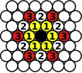
Figure 1: The interactions in the lattice model. The occupied central site (black) attracts each one of the occupied nearest-neighbor sites labelled 1 (yellow) and repels each one of the occupied third-neighbor sites labelled 3 (red). The interactions between the central site and the remaining sites vanishes. The strength of the attraction is $J_{1}$ and the strength of the repulsion is $J_{2}$.

The Hamiltonian has the form

$$H=\frac{1}{2}\sum_{\bf x}\sum_{\bf x^{\prime}}\hat{\rho}({\bf x})V({\bf x}-{\bf x}^{\prime})\hat{\rho}({\bf x^{\prime}})-\sum_{\bf x}\mu\hat{\rho}({\bf x}),$$ (1)

where $\hat{\rho}({\bf x})=1(0)$ when the site ${\bf x}$ is (is not) occupied. The interaction energy between the occupied sites ${\bf x}$ and ${\bf x}+\Delta{\bf x}$ is given by

$$V(\Delta{\bf x})=\sum_{i=1}^{3}\Big{[}-J_{1}\Big{(}\delta^{Kr}(\Delta{\bf x}+{\bf e}_{i})+\delta^{Kr}(\Delta{\bf x}-{\bf e}_{i})\Big{)}$$ (2)

$$+J_{2}\Big{(}\delta^{Kr}(\Delta{\bf x}+2{\bf e}_{i})+\delta^{Kr}(\Delta{\bf x}-2{\bf e}_{i})\Big{)}\Big{]}.$$

$-J_{1}$ and $J_{2}$ represent the attraction well and the repulsion barrier respectively, and $\delta^{Kr}({\bf x})=1$ for ${\bf x}={\bf 0}$, while $\delta^{Kr}({\bf x})=0$ for ${\bf x}\neq{\bf 0}$.

The probability of a particular microscopic state $\{\hat{\rho}({\bf x})\}$ ($\{\hat{\rho}({\bf x})\}$ denotes the values of $\hat{\rho}({\bf x})$ at all the lattice sites) has the form

$$p[\{\hat{\rho}({\bf x})\}]=\Xi^{-1}\exp(-\beta H[\{\hat{\rho}({\bf x})\}]),$$ (3)

where $\beta=1/(k_{B}T)$ and $k_{B}$ is the Boltzmann constant. The grand potential is expressed in terms of the grand statistical sum

$$\Xi=\sum_{\{\hat{\rho}({\bf x})\}}\exp(-\beta H[\{\hat{\rho}({\bf x})\}])$$ (4)

in the standard way

$$\Omega=-k_{B}T\ln\Xi=-pa_{0}L^{2}=\langle H\rangle-TS=U-TS-\mu\langle N\rangle,$$ (5)

where $a_{0}=\sigma^{2}\sqrt{3}/2$ is the area per lattice site, $p$ is 2d pressure, $\langle N\rangle$ is the average number of particles, $S$ is the entropy, and the internal energy is $U=\langle H+\mu N\rangle$.

The probability of the state $\{\hat{\rho}({\bf x})\}$ for $\mu=\tilde{V}(0)/2-\Delta\mu$ is the same as the probability of the state $\{1-\hat{\rho}({\bf x})\}$ for $\mu=\tilde{V}(0)/2+\Delta\mu$ Pȩkalski et al. (2013), where

$$\tilde{V}(0)=\sum_{\bf x}V({\bf x})=6(J_{2}-J_{1}).$$ (6)

Because of the above property, the phase diagram is symmetric with respect to the symmetry axis $\mu=\tilde{V}(0)/2=3(J_{2}-J_{1})$.

We choose $J_{1}$ as the energy unit, and introduce the notation $X^{*}=X/J_{1}$ for any quantity $X$ with dimension of energy, in particular

$$T^{*}=k_{B}T/J_{1},\quad J^{*}=J_{2}/J_{1},\quad\mu^{*}=\mu/J_{1},\quad H^{*}=H/J_{1}.$$ (7)

III The ground state

The grand potential for $T=0$ reduces to the minimum of $H^{*}[\{\hat{\rho}(x)\}]/L^{2}$. The stability regions of the homogeneous and various periodic phases on the $(J^{*},\mu^{*})$ plane were obtained by a direct calculation of $H^{*}[\{\hat{\rho}(x)\}]/L^{2}$. Two phases can coexist when $H^{*}[\{\hat{\rho}(x)\}]/L^{2}=-p^{*}$ in these phases takes the same value. The ground state (GS) and the structure of the stable phases are shown in Fig.2 and 3. For weak repulsion the vacuum and the fully occupied lattice coexist for $\mu^{*}=3J^{*}-3$. For $J^{*}>1/2$ the stability regions of the two phases are separated by the region of stability of periodic structures. The topology of the ground state is similar to the one found before in the 1d version of the model Pȩkalski et al. (2013), except that the stability region of the periodic phase splits into stability regions of several periodic phases: hexagonally ordered clusters of rhomboidal (OR) or hexagonal (HC) shape, the stripe (lamellar) phase (L) and hexagonally ordered rhomboidal (RB) or hexagonal (HB) bubbles. By the model symmetry, the bubble phases are “negatives“ (i.e. $\hat{\rho}({\bf x})\to 1-\hat{\rho}({\bf x})$) of the cluster phases.

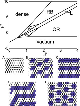
Figure 2: Ground state of the model. $\mu^{*}$ and $J^{*}$ denote the chemical potential and the third-neighbor repulsion respectively, both in units of the nearest-neighbor attraction. The structures of the stable phases are shown in the panels A-E, with: A) vacuum, B) ordered rhomboidal clusters (OR), C) and D) lamellar phase (L), E) hexagonal clusters (HC). Dense phase, hexagonal bubble phase (HB) and rhomboidal bubble phase (RB) are ”negatives“ of the phases a), b) and c) respectively, i.e. the occupied sites are replaced by the empty ones and vice versa. The symmetry line is given by $\mu^{*}=3J^{*}-3$. Configurations stable at the coexistence lines are shown in Fig. 3.

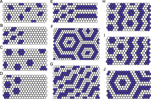
Figure 3: Examples of the ground state structures stable at the coexistence lines. Left panels: vacuum - OR phase coexistence (a-b) and vacuum - HC phase coexistence (c-d). Central panels: OR - lamellar phase coexistence. Right panels: HC - lamellar phase coexistence.

For $J^{*}>1/2$ the ground state is strongly degenerated at the coexistence lines, and the entropy per lattice site does not vanish. This can be easily shown for the coexistence between the vacuum and the OR or HC phases. In the vacuum $H^{*}=0$. The change of $H^{*}[\{\hat{\rho}({\bf x})\}]$ when a single rhomboidal or hexagonal cluster appears in the vacuum is $-5-4\mu^{*}$ or $-12+3J^{*}-7\mu^{*}$, respectively. For $\mu^{*}=-5/4$ or $\mu^{*}=(-12+3J^{*})/7$ the Hamiltonian does not change if an arbitrary number of noninteracting rhomboidal or hexagonal clusters appears in the system. The clusters do not interact if the distance between them is sufficiently large. There are no more restrictions on the positions and orientations of the clusters in the states with $H^{*}=0$ at the vacuum - OR and vacuum - HC phase coexistences (Fig.3a,c). For this reason the entropy per lattice site does not vanish. Note that the surface tension between the vacuum and the OR phases as well as between the vacuum and the HC phases vanishes, because $H^{*}=0$ when the interface between the two phases is present (Fig.3b,d). For $-5-4\mu^{*}<0$ and $-12+3J^{*}-7\mu^{*}<0$ the OR and HC phases respectively are more stable than the vacuum. In these phases the noninteracting clusters are packed as densely as possible (Fig.2 b and e).

The HC and OR phases coexist with the lamellar phase for $\mu^{*}=(13J^{*}-14)/5$ and $\mu^{*}=3J^{*}-7/2$ respectively. Note that $p^{*}$ takes the same value in the lamellar phase shown in Fig.2c, and in the zig-zag lamellar phase shown in Fig.2d. There are many configurations of the zig-zag stripes having thickness 2 in one of the lattice directions and separated by empty regions of the same shape (Fig.2 d). Thus, in the stability region of the lamellar phase the GS is degenerated. The zig-zag lamellas are discussed in more detail in Ref.Almarza et al. (2014).

At the coexistence between the lamellar and the ordered cluster phases there exists a large number of disordered states with the same value of $p^{*}$ as for the two coexisting ordered phases. Characteristic examples of such states are shown in Fig.3 e-j. Note that these states include the interface between the ordered cluster and the lamellar phases (Fig.3 e,i). In Fig.3g closely packed zig-zag clusters of different length are present. The thickness of the clusters in direction ${\bf e}_{3}$ is 2 except at the two opposing vertices where the thickness is 1. In Fig.3f,j the clusters are surrounded by lamellar rings. Structures with a few closely packed clusters surrounded by one or a few lamellar rings are stable too. All the clusters, layers or rings are packed as densely as possible under the constraint that the neighboring objects do not repel each other. More precisely, the polygons obtained by surrounding the clusters or stripes by a single layer of empty sites must cover the whole lattice. This requirement follows from the negative value of the grand potential per site in the L, HC and OR phases. We call the phase stable along the coexistence between the lamellar and the HC or OR phases a ’molten lamella’. The GS at the HC - OR coexistence, $\mu^{*}=(36J^{*}-49)/8$, is not degenerated.

The degeneracy of the GS at the phase coexistence and the vanishing surface tension are closely related. An arbitrary number of interfaces can appear when the surface tension vanishes. As a result, the number and the size of the droplets of the coexisting phases can be arbitrary. This leads to disordered states that can be considered as fluids of clusters or stripes. At $T^{*}=0$ these disordered phases are stable only at the phase coexistence, i.e. for a single value of the chemical potential for given interaction strength.

IV MF approximation

We consider stable or metastable structures with densities periodic in space. For the position-dependent density $\bar{\rho}({\bf x})$ the mean-field acting on the site ${\bf x}$ has the form

$$h({\bf x})=-\sum_{{\bf x^{\prime}}}V({\bf x}-{\bf x^{\prime}})\bar{\rho}({\bf x^{\prime}}),$$ (8)

where the interaction potential $V$ is defined in Eq.(2). The MF grand potential is

$$\Omega_{MF} = \frac{1}{2}\sum_{{\bf x}_{1}}\sum_{{\bf x}_{2}}\bar{\rho}({\bf x}_{1})\bar{\rho}({\bf x}_{2})V({\bf x}_{1}-{\bf x}_{2})+\sum_{\bf x}f_{h}(\bar{\rho}({\bf x}))-\mu\sum_{\bf x}\bar{\rho}({\bf x}),$$ (9)

where

$$f_{h}(\bar{\rho}({\bf x}))=k_{B}T\Big{[}\bar{\rho}({\bf x})\ln(\bar{\rho}({\bf x}))+(1-\bar{\rho}({\bf x}))\ln(1-\bar{\rho}({\bf x}))\Big{]}.$$ (10)

The grand potential (9) assumes a minimum for $\bar{\rho}$ which satisfies the self-consistent equation Ciach (2011a); Pȩkalski et al. (2013)

$$\bar{\rho}({\bf x})=\frac{e^{\beta(h({\bf x})+\mu)}}{1+e^{\beta(h({\bf x})+\mu)}}.$$ (11)

IV.1 The structure of the disordered phase

The structure factor in the disordered phase (with $\bar{\rho}=const.$) is obtained from the relations $S({\bf k})=\tilde{G}({\bf k})/\bar{\rho}$ and $\tilde{G}({\bf k})=1/\tilde{C}({\bf k})$ Evans (1979). In MF $\tilde{G}_{MF}({\bf k})=1/\tilde{C}_{MF}({\bf k})$, where

$$\tilde{C}_{MF}({\bf k})=\frac{\delta^{2}\beta\Omega_{MF}}{\delta\tilde{\rho}({\bf k})\delta\tilde{\rho}(-{\bf k})}=\beta\tilde{V}({\bf k})+\frac{1}{\bar{\rho}(1-\bar{\rho})}.$$ (12)

In the above $\tilde{\rho}({\bf k})=\sum_{\bf x}\rho({\bf x})e^{i{\bf k}\cdot{\bf x}}$ and

$$\beta\tilde{V}({\bf k})=\sum_{\bf x}\beta V({\bf x})e^{i{\bf k}\cdot{\bf x}}=$$

$$2\beta^{*}\Big{[}J^{*}\Big{(}\cos(2k_{1})+\cos(2k_{2})+\cos(2(k_{1}-k_{2}))\Big{)}-\cos k_{1}-\cos k_{2}-\cos(k_{1}-k_{2})\Big{]}$$ (13)

is the interaction potential in the Fourier representation. In the case of the triangular lattice ${\bf k}\equiv(k_{1},k_{2})=k_{1}{\bf f}_{1}+k_{2}{\bf f}_{2}$, and ${\bf x}\cdot{\bf y}$ is the standard scalar product in $\mathbb{R}^{2}$. The unit vectors of the dual lattice satisfy ${\bf f}_{i}\cdot{\bf e}_{j}=\delta^{Kr}_{ij}$ and $|{\bf f}_{i}|=2/\sqrt{3}$.

The maximum of the structure factor $S({\bf k})$ corresponds to the minimum of $\tilde{V}({\bf k})$. For $J^{*}<1/4$ the function given by Eq.(IV.1) assumes the minimum for ${\bf k}={\bf 0}$, whereas for $J^{*}\geq 1/4$ the minimum occurs for $k_{1}=2k_{2}=k_{b}$ with

$$k_{b}=2\arccos\Big{(}\frac{J^{*}+\sqrt{J^{*2}+2J^{*}}}{4J^{*}}\Big{)}.$$ (14)

(In Ref.Ciach (2011a) this extremum of $\tilde{V}({\bf k})$ was overlooked.) By symmetry of the lattice there are two other minima of the same depth. Thus, $\tilde{V}({\bf k})$ takes the global minima for the wavevectors

$${\bf k}_{b}^{(i)}=k_{b}{\bf e}_{i}.$$ (15)

We used the relations ${\bf e}_{1}={\bf f}_{1}+\frac{1}{2}{\bf f}_{2}$ and ${\bf e}_{2}={\bf f}_{2}+\frac{1}{2}{\bf f}_{1}$. Note that the characterisitc length $2\pi/k_{b}$ is noninteger. Thus, the period of damped oscillations in the correlation function is incommensurate with the lattice. Similar result was obtained by the exact transfer matrix method for the 1d version of our model Pȩkalski et al. (2013). In Figs.4 and 5 we show the correlation function $G_{MF}$ in Fourier and real-space representation for $J^{*}=3$ and $J^{*}=1/4$ respectively.

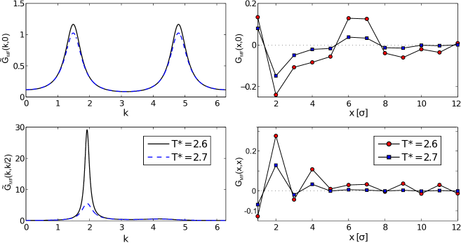
Figure 4: The correlation function for $J^{*}=3$ and $\rho^{*}=0.5$. Red circles and solid lines correspond to $T^{*}=2.6$ while blue squares and dashed lines to $T^{*}=2.8$. Left column: G in Fourier space; top panel: $\tilde{G}_{MF}(k,0)$, bottom panel: $\tilde{G}_{MF}(k,k/2)$. Right column: G in real space; top panel: $G_{MF}(x,0)$, i.e. for points ${\bf x}=x{\bf e}_{1}$, and bottom panel: $G_{MF}(x,x)$, i.e. for points ${\bf x}=x{\bf e}_{1}+x{\bf e}_{2}$. The temperature of the $\lambda$- line is $T^{*}_{\lambda}=2.575$.

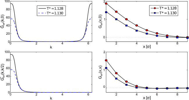
Figure 5: The correlation function for $J^{*}=1/4$ and $\rho^{*}=0.5$. Red circles and black solid lines correspond to $T^{*}=1.128$ while blue squares and dashed lines to $T^{*}=1.13$. Left column: G in Fourier space; top panel: $\tilde{G}_{MF}(k,0)$, bottom panel: $\tilde{G}_{MF}(k,k/2)$. Right column: G in real space; top panel: $G_{MF}(x,0)$, i.e. for points ${\bf x}=x{\bf e}_{1}$, and bottom panel: $G_{MF}(x,x)$, i.e. for points ${\bf x}=x{\bf e}_{1}+x{\bf e}_{2}$. The temperature of the $\lambda$- line is $T^{*}_{\lambda}=1.124$.

IV.2 Boundary of stability of the disordered phase

The disordered phase is unstable if the grand potential decreases when the density wave with an infinitesimal amplitude and some wavevector ${\bf k}$ appears, i.e. when $\tilde{C}_{MF}({\bf k})<0$. The boundary of stability of the disordered phase is given by $\tilde{C}_{MF}({\bf k}_{b})=0$. For $k_{b}=0$ and $k_{b}>0$ it corresponds to the spinodal and the $\lambda$-line respectively. From Eq.(12) we obtain the explicit expression for the boundary of stability of the disordered phase

$$T^{*}_{\lambda}=-\tilde{V}^{*}({\bf k}_{b})\rho(1-\rho).$$ (16)

In the density waves that destabilize the disordered phase the density oscillates in the principal directions of the lattice (see (15)). In the case of the lamellar structure the layers of constant density are perpendicular to either one of the unit lattice vectors ${\bf e}_{i}$ (three-fold degeneracy). In the case of the hexagonal structure the density is a superposition of 3 planar density waves in the principal lattice directions.

The shape of the $\lambda$-line in the $(\rho,T^{*})$ variables is the same as the shape of the spinodal line of the phase separation, except that the temperature scale is given by $-\tilde{V}({\bf k}_{b})$ rather than by $-\tilde{V}({\bf 0})$. This property is common for different forms of the SALR potential Archer (2008); Ciach (2008); Pȩkalski et al. (2013). However, in $(\mu^{*},T^{*})$ variables the shapes of the spinodal and the $\lambda$-lines differ significantly from each other. Moreover, the shape of the $\lambda$-line depends on $J^{*}$ (Fig.6). For $J^{*}<1/4$ the two branches of the spinodal form a cusp. On the low-$T^{*}$ side of these lines there are two minima of $\Omega_{MF}^{*}$, corresponding to the gas and liquid phases. For $J^{*}>1/4$ the two branches form a loop for high $T^{*}$. Inside the loop the grand potential assumes a minimum for periodic structures. For increasing $J^{*}$ the size of the loop increases, and for $J^{*}>1$ the gas- and liquid branches of the instability line disappear. Similar shapes were obtained in the one-dimensional lattice model Pȩkalski et al. (2013) and in the three-dimensional continuous model Barbosa (1993). Thus, the above evolution of the MF lines of instability for increasing repulsion seems to be a generic property, independent of the particular shape of the SALR potential and dimensionality of the system. Note that for $J^{*}>1/4$ we obtain instability with respect to periodic ordering for high $T^{*}$ in MF, whereas for $T^{*}=0$ the periodic phases appear only for $J^{*}>1/2$. Thus, for $1/4<J^{*}<1/2$ gas and liquid phases are stable for low $T^{*}$, periodic structures occur for intermediate $T^{*}$, and for high $T^{*}$ a disordered phase is stable. Phase separation for low $T^{*}$ and periodic ordering for high $T^{*}$ was observed before for different forms of the SALR potential for moderate repulsion in MF theories Pȩkalski et al. (2013); Andelman et al. (1987); Archer et al. (2008).

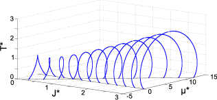
Figure 6: MF lines of instability (solid) of the homogeneous phase in the $(\mu^{*},T^{*})$ variables for a range of $J^{*}$. We used $\partial\Omega_{MF}/\partial\rho=0$, (9) and (16).

IV.3 First-order transitions

We solve Eq.(11) numerically by iterations with initial states of different symmetries and periods, and next compare the MF grand potential (9) per lattice site for the obtained metastable structures. We assume PBC and consider different values of $L$. This way structures with periods $L/n$ where $n$ is integer can be generated. We find very large number of metastable states, especially for high $T^{*}$, where the order is weak (small amplitude of the density oscillations). To overcome this problem we assume that when the amplitudes of the density oscillations in the periodic phases are small, the density has the form

$$\rho_{p}({\bf x})=\rho_{0}+\delta\rho_{p}+\Phi_{p}g_{p}({\bf x}).$$ (17)

In the above $\rho_{0}$ is the position-independent density corresponding to the extremum of $\Omega_{MF}$ for given $\mu^{*}$ and $T^{*}$. The $\delta\rho_{p}$ is the shift of the average density in the periodic phase $p$, and $g_{p}({\bf x})$ is the normalized periodic function with the symmetry of the corresponding $p$ phase, where $p=l,h$ for the lamellar and the hexagonal phase respectively. For the densities of the form (17) the excess grand potential,

$$\Delta\Omega_{p}[\rho_{p}]=\Omega_{MF}[\rho_{p}]-\Omega_{MF}[\rho_{0}],$$ (18)

is a function of $\delta\rho_{p}$ and $\Phi_{p}$ (see Eq.(9)). It takes a minimum for $\delta\rho_{p}$ and $\Phi_{p}$ corresponding to a stable or a metastable phase $p$. We limit ourselves to $\delta\rho_{p}\to 0$ and $\Phi_{p}\to 0$, and from the conditions $\partial\Delta\Omega_{p}/\partial\delta\rho_{p}=0=\partial\Delta\Omega_{p}/\partial\Phi_{p}$ obtain the approximate values of $\delta\rho_{p}$ and $\Phi_{p}$, and of the excess grand potential in the lamellar and hexagonal phases. Next, from $\Delta\Omega_{h}=0$ and $\Delta\Omega_{h}=\Delta\Omega_{l}$ we obtain the transitions between the disordered and hexagonal, and between the hexagonal and the lamellar phases respectively. These transition lines are shown as dashed lines in Fig.7. Some details of the calculation are given in Appendix.

The phase diagram obtained in the MF approximation described above is presented in Fig. 7 for $J^{*}=3$. F, H, OR, L₁ and L₂ denote the disordered fluid, the high-$T^{*}$ hexagonal phase, the ordered rhombus, and the low-$T^{*}$ and high-$T^{*}$ lamellar phases respectively. The MF density distribution in the H and L₂ phases is shown in Fig. 8, and the structure of the OR and L₁ phases for $T^{*}\to 0$ is shown in Fig.2b and Fig.2c,d respectively. In the H phase the clusters form a hexagonal pattern, but in contrast to the OR phase the orientation of the long axes of the rhombuses is not fixed. The OR phase can be present only in the case of small asymmetric clusters, i.e. for large repulsion. For $J^{*}=1$ (hence for $\int d{\bf r}V(r)=0$) hexagonal clusters appear for $T^{*}=0$ (Fig. 2 e) and only positional ordering of the clusters can occur. In the L₂ phase the orientation of the lamellas differs from the ground-state orientations, and agrees with the orientation of the density waves that destabilize the homogeneous phase. Beacuse of a very large number of metastable structures characterized by very similar values of the grand potential, it is likely that some details of the phase diagram are not reproduced in Fig.7 with full precision.

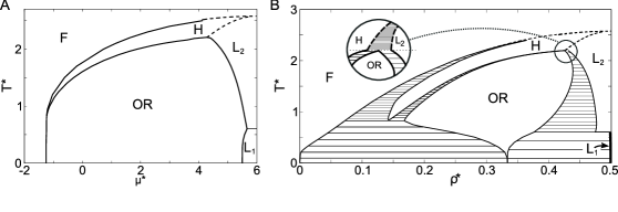
Figure 7: Mean-field phase diagram for $J^{*}=3$ in ($\mu^{*},T^{*}$) (Panel A) and ($\rho^{*},T^{*}$) (Panel B) variables. F, H, OR, L₁ and L₂ denote disordered fluid, hexagonal phase, ordered rhombuses and low- and high temperature lamellar phases respectively. Typical microstates of the OR and L₁ phases are shown in Figs. 2b and 2c,d respectively. MF density profiles in the phases H and L₂ are shown in Fig.8. The L₁ lamellar phase is stable for $T^{*}<0.65$ and $\rho\approx 0.5$ (the density interval is within the thickness of the line). When temperature rises ($T^{*}>0.65$), the L₂ phase (see Fig.8b) becomes stable. The density ranges of the two-phase regions for temperatures $T^{*}>2$ (dashed lines) are also within the thickness of the line.

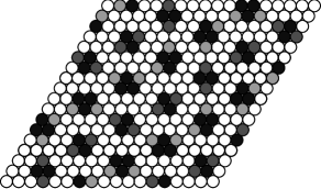
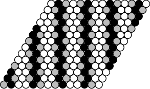
Figure 8: A: Structure of the hexagonal phase H for $J^{*}=3$, $T^{*}=0.925$ and $\rho^{*}=0.15364$. Site colors represent different ranges of probability for a particle to occur at the given site, namely: white - $(0,0.065)$, light gray - $(0.206,0.213)$ , dark gray - $(0.37,0.4)$, black - $(0.5,0.57)$. B: Structure of the lamellar phase L₂ for $J^{*}=3$, $T^{*}=1$ and $\rho^{*}=0.4905$. Sites colors represent different ranges of probability for a particle to occur at the given site, namely: white - $(0,0.045)$, light gray - $(0.6758,0.676)$, black - $0.9955$.

V Beyond Mean Field

In MF the self-assembled clusters and stripes are present only in the ordered phases, and for $T\to 0$ the density of the disordered phase at the coexistence with the OR phase is very small. This is because in the case of delocalized clusters the average density is position independent, and the repulsion contribution to the mean-field grand potential for large position-independent density is large (see (9)). In the case of rhomboidal clusters separated by distances larger than the range of the repulsion, however, the repulsion contribution to the internal energy is absent. Therefore for low $T^{*}$ the density of the disordered phase at the coexistence with the ordered cluster phase is significantly underestimated in the mean-field approximation. In sec.5a we take into account the degeneracy of the GS and present a semi-quantitative analysis of the disordered cluster fluid for $\beta^{*}(5+4\mu^{*})\to 0$ and $\beta^{*}\gg 0$.

For high $T^{*}$ thermal fluctuations destroy the periodic order, and the stability region of the disordered phase enlarges compared to the MF results. Based on the results obtained earlier for similar models Pȩkalski et al. (2013); Archer et al. (2008); Imperio and Reatto (2006) we expect that the phases with small amplitude of the density oscillations posses only short-range order beyond MF. We thus expect locally hexagonal arrangement of clusters instead of the H phase and locally lamellar order instead of the L₂ phase for $T^{*}>1.5$. According to the Brazovskii theory Brazovskii (1975), the order-disorder transition to a lamellar phase is fluctuation-induced first order in off-lattice systems. On various lattices, however, either first order or continuous order-disorder transition to the periodically ordered phase may occur Ciach and Stell (2003). We determine the order of this transition, and calculate the correlation function in the field-theoretic formalism in sec. 5b.

V.1 The effect of the degeneracy of the ground state on the phase diagram for $T^{*}>0$

For $J^{*}>1$ and the state points that satisfy $\beta^{*}(5+4\mu^{*})\to 0^{-}$ all the microscopic states consisting of $N$ noninteracting rhombuses are almost equally probable, since the probability of such states is proportional to $\exp[\beta^{*}(5+4\mu^{*})N]\approx 1$, and for $\beta^{*}\gg 0$ other states (with $H^{*}>0$) are rare. We can obtain an upper bound for the grand potential of the cluster fluid by considering a subset of all such microscopic states. Let us consider the sublattice shown in Fig.9a. The sites of the sublattice can be empty, or occupied by noninteracting rhombuses.

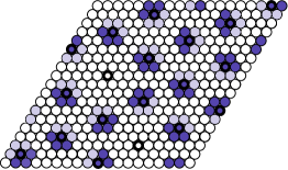
Figure 9: A: The black solid circles represent sites of the sublattice considered in sec. 5 A. The corresponding sites are occupied if they belong to a rhomboidal cluster. The dark blue color indicates one of the possible orientations of the rhomboidal clusters. B: A portion of the ($\rho^{*}$,$T^{*}$) phase diagram for $J^{*}=3$ with the coexistence region between the cluster fluid (CF) and the OR phase (dash-dotted lines) estimated on the basis of the sublattice shown in panel A.

There are 6 possible orientations of the rhombuses at each site of the sublattice and the number of sublattice sites is $L^{2}/19$. The sublattice sites are occupied or empty independently of one another, and the grand potential and the average density can be obtained immediately,

$$\Omega^{*}/L^{2}=-\frac{T^{*}}{19}\ln\Bigg{(}1+6e^{\beta^{*}(5+4\mu^{*})}\Bigg{)}$$ (19)

and

$$\bar{\rho}=\frac{4}{19}\frac{6e^{\beta^{*}(5+4\mu^{*})}}{1+e^{\beta^{*}(5+4\mu^{*})}}.$$ (20)

For $\beta^{*}(5+4\mu^{*})=0$ we obtain $\bar{\rho}\approx 0.18$. This gives the order of magnitude of the density in the cluster fluid for $\mu^{*}=-5/4$. We compare the grand potential per lattice site, Eq. (19), with $\Omega_{MF}^{*}/L^{2}$ calculated in the MF approximation for the OR phase. This way we obtain a rough estimate of the coexistence region between the cluster fluid and the OR phase. The corresponding portion of the phase diagram is shown in Fig.9b. Since only a subset of the microscopic states was considered and in the disordered phase the positions of the rhombuses are not restricted to the sublattice sites, the stability region of the CF phase is expected to be larger than shown in Fig.9b. By analogy we expect that the molten lamella phase found at the coexistence between the OR and lamellar phases for $T^{*}=0$ will remain stable for $T^{*}>0$ for the state points that satisfy $\beta^{*}(2\mu^{*}+5-6J^{*})\to 0$.

V.2 The effect of mesoscopic fluctuations on the correlation function

In this subsection we investigate the effect of mesoscopic fluctuations on the structure of the disordered phase in the field-theoretic formalism. The grand potential (5) in the coarse-grained description Ciach and Patsahan (2012); Ciach (2011b, 2008) is approximated by

$$\beta\Omega\approx-\ln\Big{(}\int D\rho e^{-\beta\Omega_{MF}[\rho]}\Big{)}=\beta\Omega_{MF}[\bar{\rho}]-\ln\Big{(}\int D\phi e^{-\beta H_{f}[\bar{\rho},\phi]}\Big{)}$$ (21)

where

$$\beta H_{f}[\bar{\rho},\phi]=\beta\Omega_{MF}[\bar{\rho}+\phi]-\beta\Omega_{MF}[\bar{\rho}],$$ (22)

$\phi({\bf x})$ is a mesoscopic fluctuation of the density, and the average density denoted by $\bar{\rho}({\bf x})$ satisfies the extremum condition

$$\frac{\delta\beta\Omega}{\delta\rho({\bf x})}=\frac{\delta\beta\Omega_{MF}}{\delta\rho({\bf x})}+\langle\frac{\delta\beta H_{f}}{\delta\rho({\bf x})}\rangle_{f}=0.$$ (23)

In derivation of the above Eq.(21) was used, and $\langle...\rangle_{f}$ denotes averaging with the probability $\propto\exp(-\beta H_{f})$. The MF approximation is valid when the second term on the RHS of (23) is negligible. In this theory $\rho({\bf x})$ is the mesoscopic density, i.e. the density averaged over a mesoscopic region around each point ${\bf x}$. In Eq.(21) $\Omega_{MF}[\rho]$ describes the grand potential of a system whose mesoscopic density is constrained to have the form $\rho({\bf x})$ Ciach and Patsahan (2012); Ciach (2011b, 2008). In our approximation the explicit expression for $\Omega_{MF}[\rho]$ is given in Eq.(9). We limit our attention to the disordered phase with $\bar{\rho}({\bf x})=\bar{\rho}=const.$. The correlation function in Fourier representation, $\langle\tilde{\phi}({\bf k})\tilde{\phi}(-{\bf k})\rangle=\tilde{G}({\bf k})=1/\tilde{C}({\bf k})$, can be obtained from the equation

$$\tilde{C}({\bf k})=\frac{\delta^{2}\beta\Omega}{\delta\tilde{\rho}({\bf k})\delta\tilde{\rho}(-{\bf k})}=\tilde{C}_{MF}({\bf k})+\langle\frac{\delta^{2}\beta H_{f}}{\delta\tilde{\rho}({\bf k})\delta\tilde{\rho}(-{\bf k})}\rangle_{f}-\langle\frac{\delta\beta H_{f}}{\delta\tilde{\rho}({\bf k})}\frac{\delta\beta H_{f}}{\delta\tilde{\rho}(-{\bf k})}\rangle_{f}^{conn}$$ (24)

where $\langle AB\rangle_{f}^{conn}=\langle AB\rangle_{f}-\langle A\rangle_{f}\langle B\rangle_{f}$.

We write (22) in the form

$$\beta H_{f}[\bar{\rho},\phi]=\frac{1}{2}\int d{\bf k}\tilde{\phi}({\bf k})\tilde{C}(\bar{\rho},{\bf k})\tilde{\phi}(-{\bf k})+\Delta H_{f},$$ (25)

neglect the correction term $\Delta H_{f}$ and approximate the $n-$th functional derivative of $\Omega$ for $n\geq 3$ by the corresponding derivative of $\Omega_{MF}$. This way we obtain the self-consistent Gaussian approximation for the correlation function $\tilde{G}({\bf k})$. In this self-consistent approximation Eq.(24) takes the form

$$\tilde{C}({\bf k})=\beta\tilde{V}({\bf k})+A_{2}+\frac{A_{4}}{2}\int\frac{d{\bf k}^{\prime}}{(2\pi)^{d}\tilde{C}({\bf k}^{\prime})}-\frac{A_{3}^{2}}{2}\int\frac{d{\bf k}^{\prime}}{(2\pi)^{d}\tilde{C}({\bf k}^{\prime})\tilde{C}({\bf k}^{\prime}+{\bf k})}$$ (26)

where

$$A_{n}=\frac{d^{n}\beta f_{h}(\rho)}{d\rho^{n}}$$ (27)

and for the lattice models $f_{h}(\rho)$ is given in Eq.(10).

Here we limit ourselves to $\rho\approx 1/2$ where $A_{3}\approx 0$. For $A_{3}=0$ we obtain from (26) the Brazovskii approximation Brazovskii (1975),

$$\tilde{C}({\bf k})=\beta\tilde{V}({\bf k})+A_{2}+a(\beta^{*},\rho)$$ (28)

where

$$a(\beta^{*},\rho)=\frac{A_{4}}{2}\int\frac{d{\bf k}}{(2\pi)^{d}(\beta\tilde{V}({\bf k})+A_{2}+a(\beta^{*},\rho))}.$$ (29)

We numerically solve Eq.(29) for $\rho=1/2$ and a range of $T^{*}$. The maximum of $\tilde{G}({\bf k})$ is compared with the MF result in Fig.10.

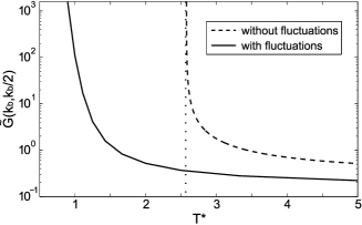
Figure 10: The maximum of the correlation function in Fourier representation, $\tilde{G}(k_{b},k_{b}/2)$ for $\rho=1/2$ as a function of the reduced temperature $T^{*}=k_{B}T/J_{1}$. Dashed and solid lines correspond to the MF and the Brazovskii-type approximation respectively. In the MF approximation $\tilde{G}(k_{b},k_{b}/2)$ is approximated by $\tilde{G}_{MF}(k_{b},k_{b}/2)$ (see sec. 4 A) which diverges at the $\lambda$-line $T^{*}=2.575$, while in a presence of fluctuations $\tilde{G}(k_{b},k_{b}/2)$ diverges at $T^{*}=0$.

The boundary of stability of the disordered phase in this approximation should be given by $\tilde{C}({\bf k}_{b})=0$. However, in a 2d system the integral in Eq.(29) diverges for the state points for which $\tilde{C}({\bf k}_{b})=0$. Thus, the assumption that LHS of Eq. (28) vanishes, leads to divergent RHS for $T^{*}>0$. This indicates the absence of the instability of the disordered phase with respect to small-amplitude density waves for $T^{*}>0$, and a fluctuation-induced first-order phase transition is expected Brazovskii (1975). Note, however that $\tilde{G}(k_{b},k_{b}/2)$ is very large, $\sim 10^{2}$ for $T^{*}=1$ and very quickly increases for $T^{*}<1$ (see Fig.10). The correlation function in the Brazovskii approximation is shown in Fig.11 for $\rho=1/2$ and two temperatures, $T^{*}=1$ and $T^{*}=2.7$.

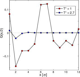
Figure 11: The correlation function along the lattice direction, i.e. for the sites ${\bf x}=x{\bf e}_{1}$ for $\rho=1/2$ and two temperatures, $T^{*}=1$ (red circles) and $T^{*}=2.7$ (blue squares) in the Brazovskii approximation.

VI Summary and discussion

We have introduced a triangular lattice model for self-assembly of nanoparticles or proteins on surfaces, interfaces or membranes. We have assumed nearest-neighbor attraction and third-neighbor repulsion. Such interaction ranges were found for example for lysozyme molecules in water Shukla et al. (2008). The advantage of the lattice model is the possibility of detailed investigation of the ground state, where the disordering effect of thermal motion is absent. We have found stability regions of periodically distributed clusters, bubbles or stripes. A very interesting property of the ground state is its strong degeneracy at the coexistence between ordered phases of different symmetry. The entropy per site at the coexistence between different ordered phases does not vanish. We identify the disordered states stable at the phase coexistence between vacuum and hexagonally ordered clusters (Fig.3a,c) with a disordered cluster fluid. The disordered states stable at the coexistence between the ordered clusters and stripes (Fig.3e-j) correspond to a disordered phase called molten lamella. The structures stable at the above phase coexistences include the interface between the two phases. Thus, the surface tension vanishes.

The vanishing surface tension and the strong degeneracy of the GS at the phase coexistence as well as an ultra-low surface tension for $T^{*}>0$ were observed previously in surfactant solutions Ciach et al. (1989); Ciach and Góźdź (2001); Gommper and Schick (1994). Here we show that the amphiphilic molecules are not necessary to obtain the vanishing surface tension at $T=0$. The surface tension vanishes when the ground state is strongly degenerated at the phase coexistence, and the stable structures include the interface. The effects of the vanishing surface tension in the case of the colloid and amphiphilic self-assembly are very similar. Namely, disordered phases with strong local inhomogeneities become stable. In the case of amphiphiles these phases are the micellar, the microelmulsion and the sponge phases, whereas in the case of the SALR potential - the cluster fluid and the molten lamella.

The degeneracy of the ground state leads to a huge number of thermodynamically stable patterns. Particularly interesting are the patterns stable in the molten lamella phase. The patterns are composed of a few motifs: clusters, stripes or rings that are surrounded by a single layer of empty sites. A transition between different stable patterns is a collective phenomenon, involving a large fraction of the particles. The information encoded in the stable patterns cannot be easily destroyed by the thermal motion when $T^{*}$ is not high.

We have determined the phase diagram for $T^{*}>0$ in the mean-field approximation. We have obtained the same sequence of the orderd periodic phases as in Ref.Archer (2008). For increasing density the stable phases are: fluid, hexagonally ordered clusters, lamellar phase and hexagonally ordered bubbles. For high $T^{*}$ the phase diagrams on the lattice and in continuum are very similar. However, on the lattice there are two lamellar phases with different orientations of the stripes w.r.t the lattice directions. For strong repulsion ($J^{*}=3$) we obtain two hexagonal phases, with and without orientational ordering of the long axes of the rhomboidal clusters. The regions occupied by the ordered phases and the extent of the two-phase regions on the $(\rho^{*},T^{*})$ phase diagram are also different than in Ref.Archer (2008). For weak repulsion ($J^{*}=1$, i.e. $\int d{\bf r}V(r)=0$) the clusters are symmetrical and there is a single haxagonal phase, as in Ref.Archer (2008).

Unfortunately, in the mean-field approximation the effect of the degeneracy of the ground state cannot be correctly described. In mean field the mesoscopic fluctuations are neglected, whereas in the SALR systems the displacements of the clusters or stripes lead to formation of the disordered cluster fluid or molten lamella. The dominant role of mesoscopic fluctuations makes the studies of the SALR systems particularly difficult. In off-lattice systems the phase diagrams obtained in the DFT Archer (2008) and in MC simulations Imperio and Reatto (2006) differ significantly from each other. The main features present on the MC and absent on the DFT phase diagram are: (i) a stability of the cluster fluid phase between the ordered cluster phase and the homogeneous fluid (ii) a reentrant melting of the ordered cluster phase for high temperatures. Similar difference between the high-$T$ part of the phase diagrams in mean-field approximation and in a presence of fluctuations was observed in the context of block copolymers when fluctuations were taken into account within field-theoretic methods Brazovskii (1975); Fredrickson and Helfand (1987); Podneks and Hamley (1996).

We expect similar differences between mean-field and exact results for the present lattice model. From our preliminary studies of the effects of fluctuations two conclusions follow: (i) the cluster fluid is stable for low $T^{*}$ up to the density $\rho=0.2$ or larger, and (ii) the transition to the lamellar phase is fluctuation-induced first order. The fluctuation-induced first-order transitions are usually very weakly first order. Moreover, the maximum of the structure factor increases to very large values for $T^{*}<0.8$, and it may be difficult to determine the order of the transition in experiment or simulation. The effects of fluctuations on the phase diagram of this model are studied in much more detail by Monte Carlo simulations in Ref.Almarza et al. (2014).

Acknowledgments The work of JP was realized within the International PhD Projects Programme of the Foundation for Polish Science, cofinanced from European Regional Development Fund within Innovative Economy Operational Programme ”Grants for innovation”. AC and JP acknowledge the financial support by the NCN grant 2012/05/B/ST3/03302. N.G.A. gratefully acknowledges financial support from the Dirección General de Investigación Científica y Técnica under Grant No. FIS2010-15502, from the Dirección General de Universi- dades e Investigación de la Comunidad de Madrid under Grant No. S2009/ESP-1691 and Program MODELICO-CM.

VII Appendix. Grand potential for weakly ordered periodic phases in MF

The normalized functions $g_{p}$ satisfy the equations

$$\frac{1}{V_{u}}\sum_{{\bf x}\in V_{u}}g_{p}({\bf x})=0$$ (30)

and

$$\frac{1}{V_{u}}\sum_{{\bf x}\in V_{u}}g_{p}^{2}({\bf x})=1.$$ (31)

In the above equations the summation is over the unit cell of the ordered structure with the area $V_{u}$. The length of the unit cell in our case is $2\pi/k_{b}$. The functions $g_{p}$ for the lamellar and hexagonal phases have the forms

$$g_{l}({\bf x})=\sqrt{2}\cos(k_{b}{\bf x}\cdot{\bf e}_{i})$$ (32)

and

$$g_{h}({\bf x})=\sqrt{\frac{2}{3}}\sum_{i=1}^{3}\cos(k_{b}{\bf x}\cdot{\bf e}_{i})$$ (33)

where $k_{b}$ is given in Eq.(14). In the case of noninteger $2\pi/k_{b}$, in order to calculate Eqs.(30) and (31), we make the approximation

$$\frac{1}{V_{u}}\sum_{{\bf x}\in V_{u}}f(k_{b}{\bf x})\simeq\int_{0}^{2\pi}\frac{dz_{1}}{(2\pi)}\int_{0}^{2\pi}\frac{dz_{2}}{(2\pi)}f({\bf z}),$$ (34)

where $z_{i}=k_{b}x_{i}$.

From the condition $\partial\Delta\Omega/\partial\delta\rho_{p}=0$ we obtain for $\Phi_{p}\ll 1$

$$\delta\rho_{p}\cong-\frac{A_{3}\Phi_{p}^{2}}{2(\beta^{*}{\tilde{V}^{*}(0)+A_{2})}},$$ (35)

where $A_{n}$ is defined in Eq.(27), and $\beta^{*}\tilde{V}^{*}(0)\rho_{0}+A_{1}-\beta^{*}\mu^{*}=0$. After some algebra we obtain the approximate expression

$$\beta^{*}\Delta\Omega_{p}^{*}=\Phi^{2}_{p}\,\,\frac{\beta^{*}\tilde{V}^{*}(\mathbf{k}_{b})+A_{2}}{2}+\Phi^{3}_{p}\,\,\frac{A_{3}\kappa_{3}^{p}}{3!}+\Phi^{4}_{p}\Big{[}\frac{A_{4}\kappa_{4}^{p}}{4!}-\frac{A_{3}^{2}}{8(\beta^{*}\tilde{V}^{*}(0)+A_{2})}\Big{]}+O(\Phi^{5}_{p}),$$ (36)

where the geometric factors are defined as $\kappa_{n}^{p}=\frac{1}{V_{u}}\sum_{V_{u}}g_{p}({\bf x})^{n}$ and take the following values $\kappa_{3}^{l}=0$, $\kappa_{4}^{l}=\frac{3}{2}$, $\kappa_{3}^{h}=\sqrt{\frac{2}{3}}$, $\kappa_{4}^{h}=\frac{5}{2}$ Ciach and Góźdź (2010). From $\partial\Delta\Omega/\partial\delta\Phi_{p}=0$ we obtain the amplitude $\Phi_{p}$, and after inserting it to (36), the value of $\beta\Delta\Omega_{p}^{*}$ for given $T^{*}$ and $\rho_{0}$.

References

- Israelachvili (2011) J. N. Israelachvili, Intermolecular and Surface Forces (Third Edition) (Academic Press, Boston, 2011).
- Shukla et al. (2008) A. Shukla, E. Mylonas, E. D. Cola, S. Finet, P. Timmins, T. Narayanan, and D. I. Sveergun, Proc. Nat. Acad. Sci. USA 105, 5075 (2008).
- Stradner et al. (2004) A. Stradner, H. Sedgwick, F. Cardinaux, W. Poon, S. Egelhaaf, and P. Schurtenberger, Nature 432, 492 (2004).
- Campbell et al. (2005) A. I. Campbell, V. J.Anderson, J. S. van Duijneveldt, and P. Bartlett, Phys. Rev. Lett 94, 208301 (2005).
- Seul and Andelman (1995) M. Seul and D. Andelman, Science 267, 476 (1995).
- Sanchez-Iglesias et al. (2012) A. Sanchez-Iglesias, M. Grzelczak, T. Altantzis, B. Goris, J. Perez-Juste, S. Bals, G. V. Tondeloo, S. H. Donaldson, B. F. Chmelka, J. N. Israelachvili, et al., ACS Nano 6, 11059 (2012).
- Lafitte et al. (2013) T. Lafitte, S. Kumar, and A. Z. Panagiotopolous, Soft Matter (2013), DOI: 10.1039/C3SM52328D.
- Scheve et al. (2013) C. S. Scheve, P. A. Gonzales, N. Momin, and J. C. Stachowiak, J. Am. Chem. Soc 135, 1185 (2013).
- Helfrich (1973) W. Helfrich, Z Naturforsch 28 c, 693 (1973).
- Dijkstra et al. (1999) M. Dijkstra, R. van Roij, and R. Evans, Phys. Rev. E 59, 5744 (1999).
- Machta et al. (2012) B. B. Machta, S. L. Veatch, and J. P. Sethna, Phys. Rev. Lett 109, 138101 (2012).
- Pergamenshchik (2012) V. M. Pergamenshchik, Phys. Rev. E 85, 021403 (2012).
- Sear and Gelbart (1999) R. P. Sear and W. M. Gelbart, J. Chem. Phys 110, 4582 (1999).
- Pini et al. (2000) D. Pini, G. Jialin, A. Parola, and L. Reatto, Chem. Phys. Lett. 327, 209 (2000).
- Imperio and Reatto (2004) A. Imperio and L. Reatto, J. Phys.:Cond. Mat 18, S2319 (2004).
- Imperio and Reatto (2007) A. Imperio and L. Reatto, Phys. Rev. E 76, 040402 (2007).
- Imperio and Reatto (2006) A. Imperio and L. Reatto, J. Chem. Phys 124, 164712 (2006).
- Pini et al. (2006) D. Pini, A. Parola, and L. Reatto, J. Phys.:Cond. Mat 18, S2305 (2006).
- Archer et al. (2007) A. J. Archer, D. Pini, R. Evans, and L. Reatto, J. Chem. Phys 126, 014104 (2007).
- Archer (2008) A. J. Archer, Phys. Rev. E 78, 031402 (2008).
- Ciach et al. (2013) A. Ciach, J. Pȩkalski, and W. T. Gozdz, Soft Matter 9, 6301 (2013).
- Kowalczyk et al. (2011) P. Kowalczyk, A. Ciach, P. A. Gauden, and A. P. Terzyk, Int. J. Colloid and Interf. Sci. 363, 579 (2011).
- Pȩkalski et al. (2013) J. Pȩkalski, A. Ciach, and N. G. Almarza, J. Chem. Phys 138, 144903 (2013).
- Almarza et al. (2014) N. Almarza, J. Pȩkalski, and A. Ciach (2014), preprint.
- Ciach (2011a) A. Ciach, J. Mol. Liquids 164, 74 (2011a).
- Evans (1979) R. Evans, Adv. Phys 28, 143 (1979).
- Ciach (2008) A. Ciach, Phys. Rev. E 78, 061505 (2008).
- Barbosa (1993) M. C. Barbosa, Phys. Rev. E 48, 1744 (1993).
- Andelman et al. (1987) D. Andelman, F. Brochard, and J.-F. Joanny, Proc. Nat. Acad. Sci. USA 84, 4717 (1987).
- Archer et al. (2008) A. Archer, Ionescu, D. Pini, and L. Reatto, J. Phys.:Cond. Mat 20, 415106 (2008).
- Brazovskii (1975) S. A. Brazovskii, Sov. Phys. JETP 41, 8 (1975).
- Ciach and Stell (2003) A. Ciach and G. Stell, Phys. Rev. Lett 91, 060601 (2003).
- Ciach and Patsahan (2012) A. Ciach and O. Patsahan, Condens. Matter Phys. 15, 23604 (2012).
- Ciach (2011b) A. Ciach, Mol. Phys 109, 1101 (2011b).
- Ciach et al. (1989) A. Ciach, J. S. Høye, and G. Stell, J. Chem. Phys 90, 1214 (1989).
- Ciach and Góźdź (2001) A. Ciach and W. T. Góźdź, Annu. Rep.Prog. Chem., Sect.C 97, 269 (2001), and references therein.
- Gommper and Schick (1994) G. Gommper and M. Schick, Self-Assembling Amphiphilic Systems, vol. 16 of Phase Transitions and Critical Phenomena (Academic Press, 1994), 1st ed.
- Fredrickson and Helfand (1987) G. H. Fredrickson and E. Helfand, J. Chem. Phys 87, 67 (1987).
- Podneks and Hamley (1996) V. E. Podneks and I. W. Hamley, Pis’ma Zh. Exp. Teor. Fiz. 64, 564 (1996).
- Ciach and Góźdź (2010) A. Ciach and W. T. Góźdź, Condensed Matter Physics 13, 23603 (2010).