Domain decomposition methods
with overlapping subdomains
for time-dependent problems

1 Introduction

Domain decomposition methods are used for the numerical solution of boundary value problems for partial differential equations on parallel computers. In the theory of domain decomposition methods, modern studies are most fully presented for stationary problems Quarteroni and Valli (1999); Toselli and Widlund (2005). Computational algorithms with and without overlap of subdomains are applied in synchronous (sequential) and asynchronous (parallel) methods.

Domain decomposition methods for unsteady problems are based on two basic approaches Samarskii et al. (2002).

1. For the numerical solution of time-dependent problems, we use the standard implicit approximation in time. Domain decomposition methods are applied to solve the discrete problem at the new time level. The number of iterations in optimal iterative methods for domain decomposition does not depend on steps of discretization in time and space.

2. To solve unsteady problems, iteration-free domain decomposition algorithms are developed. We construct a special scheme of splitting into subdomains (regionally additive schemes).

A domain decomposition scheme is defined by a decomposition of the computational domain and by specifying a splitting of the problem operator. To construct decomposition operators, it is convenient to use the partition of unity for the computational domain.

In DD methods with overlap, we introduce a function associated with each subdomain, and this function takes value between zero and one. In the extreme case, the width of overlap of subdomains is equal to the step of discretization in space. In this case, regionally additive schemes can be interpreted as non-overlapping domain decomposition schemes, where data exchange is achieved by setting proper boundary conditions for each subdomain.

Domain decomposition methods for unsteady problems include the following steps:

• Decomposition of a domain;

• Constructing operators of decomposition;

• Design of a splitting scheme;

• A study of convergence;

• Computational implementation.

These basic questions are discussed in this paper using a boundary value problem for the second-order parabolic equation as an example.

2 Standard approximation

Assume that in a bounded domain $\Omega$, a unknown function $u({\bm{x}},t)$ satisfies the following equation:

$$\frac{\partial u}{\partial t}-\sum_{\alpha=1}^{m}\frac{\partial}{\partial x_{\alpha}}\left(k({\bm{x}})\frac{\partial u}{\partial x_{\alpha}}\right)=f({\bm{x}},t),\quad{\bm{x}}\in\Omega,\quad 0<t\leq T,$$ (1)

where $k({\bm{x}})\geq\kappa>0,\ {\bm{x}}\in\Omega$. Homogeneous Dirichlet boundary conditions are applied:

$$u({\bm{x}},t)=0,\quad{\bm{x}}\in\partial\Omega,\quad 0<t\leq T.$$ (2)

The initial condition is

$$u({\bm{x}},0)=u^{0}({\bm{x}}),\quad{\bm{x}}\in\Omega.$$ (3)

Let $(\cdot,\cdot),\|\cdot\|$ be the scalar product and the norm in $L_{2}(\Omega)$, respectively:

$$(u,v)=\int_{\Omega}u({\bm{x}})v({\bm{x}})d{\bm{x}},\quad\|u\|=(u,u)^{1/2}.$$

A symmetric, positive definite, bilinear form $d(u,v)$ such that

$$d(u,v)=d(v,u),\quad d(u,u)\geq\delta\|u\|^{2},\quad\delta>0,$$

is associated with a Hilbert space $H_{d}$ equipped with the following scalar product and norm:

$$(u,v)_{d}=d(u,v),\quad\|u\|_{d}=(d(u,u))^{1/2}.$$

Suppose $t=t^{n}=n\tau,\ n=0,1,...$, where $\tau>0$ is a constant time step. A finite-dimensional space of finite elements is denoted by ${\cal V}^{h}$, and $u^{n}=u(\bm{x},t^{n})\ (u^{n}\in{\cal V}^{h})$ stands for the approximate solution at the time level $t=t^{n}$. The boundary value problem (1)–(3) is treated in the variational form:

$$\left(\frac{du}{dt},v\right)+a(u,v)=(f,v),\quad\forall v\in H^{1}_{0}(\Omega),\quad 0<t\leq T,$$ (4)

$$(u(0),v)=(u^{0},v),\quad\forall v\in H^{1}_{0}(\Omega),$$ (5)

where

$$a(u,v)=\int_{\Omega}k({\bm{x}})\ {\rm grad}\,u\ {\rm grad}\,v\ d{\bm{x}}.$$

We study the projection-difference scheme (schemes with weights) for (4), (5):

$$\left(\frac{y^{n+1}-y^{n}}{\tau},v\right)+a(\sigma y^{n+1}+(1-\sigma)y^{n},v)=(f(\sigma t^{n+1}+(1-\sigma)t^{n}),v),$$ (6)

$$(y^{0},v)=(u^{0},v),\quad\forall v\in{\cal V}^{h},\quad n=1,2,...,$$ (7)

where $\sigma$ is a number (weight). If $\sigma=0$, then the scheme (6), (7) is the explicit (Euler forward-time) scheme; for $\sigma=1$, we obtain the fully implicit (Euler backward-time) scheme; and $\sigma=0.5$ yields the averaged (the so-called Crank–Nicolson) scheme. The condition

$$(v,v)+\left(\sigma-\frac{1}{2}\right)\ \tau\ a(v,v)\geq 0,\quad\forall v\in{\cal V}^{h}$$

is necessary and sufficient for the stability of the scheme in the space $H_{a}$ Samarskii (2001); Samarskii et al. (2002).

3 Decomposition operators

To construct a domain decomposition scheme, we introduce the partition of unity for the computational domain $\Omega$ Laevsky (1987). Assume that the domain $\Omega$ consists of $p$ separate subdomains:

$$\Omega=\Omega_{1}\cup\Omega_{2}\cup...\cup\Omega_{p}.$$

Individual subdomains may be overlaped. With an individual subdomain $\Omega_{\alpha},\ \alpha=1,2,...,p$ we associate the function $\eta_{\alpha}({\bm{x}}),\ \alpha=1,2,...,p$ such that

$$\eta_{\alpha}({\bm{x}})=\left\{\begin{array}[]{cc}>0,&{\bm{x}}\in\Omega_{\alpha},\\ 0,&{\bm{x}}\notin\Omega_{\alpha},\\ \end{array}\right.\quad\alpha=1,2,...,p,$$

where

$$\sum_{\alpha=1}^{p}\eta_{\alpha}({\bm{x}})=1,\quad{\bm{x}}\in\Omega.$$

For problem (4), (5), we have

$$a(u,v)=\sum_{\alpha=1}^{p}a_{\alpha}(u,v),\quad(f,v)=\sum_{\alpha=1}^{p}(f_{\alpha},v).$$

Here

$$(f_{\alpha},v)=\int_{\Omega}\eta_{\alpha}({\bm{x}})f({\bm{x}},t)v\ d{\bm{x}}$$

and (the standard decomposition)

$$a_{\alpha}(u,v)=\int_{\Omega}\eta_{\alpha}({\bm{x}})k({\bm{x}})\ {\rm grad}\,u\ {\rm grad}\,v\ d{\bm{x}},\quad\alpha=1,2,...,p.$$

Other variants of domain decompositon operators Vabishchevich (1989) are associated with the following forms:

$$a_{\alpha}(u,v)=\int_{\Omega}k({\bm{x}})\ {\rm grad}\,u\ {\rm grad}\,(\eta_{\alpha}({\bm{x}})v)\ d{\bm{x}},$$

$$a_{\alpha}(u,v)=\int_{\Omega}k({\bm{x}})\ {\rm grad}\,(\eta_{\alpha}({\bm{x}})u)\ {\rm grad}\,v\ d{\bm{x}},\quad\alpha=1,2,...,p.$$

Let us investigate the corresponding operator-splitting schemes. From problem (4), (5), we can go to the Cauchy problem for the evolutionary equation of first order (matrix form Thomée (2006)):

$$B\frac{dy}{dt}+Ay=\varphi(t),\quad 0<t\leq T,$$ (8)

$$y(0)=y^{0}.$$ (9)

Here the mass matrix $B=B^{*}>0$, and the stiffness matrix $A=A^{*}>0$.

For (8), (9), we have the following operator splitting:

$$A=\sum_{\alpha=1}^{p}A_{\alpha},\quad\varphi=\sum_{\alpha=1}^{p}\varphi_{\alpha}$$

with (the standard decomposition)

$$A_{\alpha}=A_{\alpha}^{*}\geq 0,\quad\alpha=1,2,...,p.$$

We arrive to the symmetrized equation:

$$\frac{dw}{dt}+\widetilde{A}w=\widetilde{\varphi}(t),\quad 0<t\leq T,$$

where

$$w=B^{1/2}v,\quad\widetilde{A}=B^{-1/2}AB^{-1/2},\quad\widetilde{\varphi}=B^{-1/2}\varphi,$$

$$\widetilde{A}=\sum_{\alpha=1}^{p}\widetilde{A}_{\alpha},\quad\widetilde{A}_{\alpha}=\widetilde{A}_{\alpha}^{*}=B^{-1/2}A_{\alpha}B^{-1/2}\geq 0,\quad\alpha=1,2,...,p.$$

Now we can employ general results of the stability (correctness) theory for operator-difference schemes Samarskii (2001); Samarskii et al. (2002).

4 Splitting schemes

The investigation of domain decomposition schemes for time-dependent problems is based on consideration of the relevant splitting schemes Vabishchevich (2014). Here we highlight the case of the two-component splitting ($p=2$). In this case, we can focus on the following methods:

• the Douglas-Rachford scheme,

• the Peaceman-Rachford scheme,

• Factorized schemes,

• Symmetric scheme of componentwise splitting.

In particular, the Douglas-Rachford scheme may be written as:

$$\left(\frac{u^{n+1/2}-u^{n}}{\tau},v\right)+a_{1}(u^{n+1/2},v)+a_{2}(u^{n},v)=(f^{n+1},v),$$

$$\left(\frac{u^{n+1}-u^{n}}{\tau},v\right)+a_{1}(u^{n+1/2},v)+a_{2}(u^{n+1},v)=(f^{n+1},v),\quad\forall v\in{\cal V}^{h}.$$

The problem in the subdomain (explicit-implicit scheme) is formulated in the form:

$$(u^{n+1/2},v)+\tau a_{1}(u^{n+1/2},v)=(u^{n},v)-\tau a_{2}(u^{n},v)+\tau(f^{n+1},v),$$

$$(u^{n+1},v)+\tau a_{2}(u^{n+1},v)=(u^{n},v)-\tau a_{1}(u^{n+1.2},v)+\tau(f^{n+1},v).$$

In the domain $\Omega\setminus\bar{\Omega}_{1}$ we have the explicit scheme for computing $u^{n+1/2}$. It is sufficient to perform computations for $\partial\Omega_{1}\cap\Omega$. Next, we solve the problem in the subdomain $\Omega_{1}$ to find $u^{n+1/2}$. The calculation of $u^{n+1}$ are performed similarly.

In the more general case, we focus on factorized schemes with weights:

$$\left(\frac{u^{n+1/2}-u^{n}}{\tau},v\right)+a_{1}(\sigma u^{n+1/2}+(1-\sigma)u^{n},v)+a_{2}(u^{n},v)=(f^{n+\sigma},v),$$ (10)

$$\begin{split}&\left(\frac{u^{n+1}-u^{n}}{\tau},v\right)+a_{1}(\sigma u^{n+1/2}+(1-\sigma)u^{n},v)\\ &+a_{2}(\sigma u^{n+1}+(1-\sigma)u^{n},v)=(f^{n+\sigma},v),\quad\forall v\in{\cal V}^{h},\quad n=1,2,...,\end{split}$$ (11)

where $f^{n+\sigma}=f(\sigma t^{n+1}+(1-\sigma)t^{n})$. For $\sigma=1/2$, we obtain the Peaceman-Rachford scheme, whereas at $\sigma=1$ we have the Douglas-Rachford scheme.

The operator (matrix) form of the factorized scheme (10), (11) seems like this:

$$(B+\sigma\tau A_{1})B^{-1}(B+\sigma\tau A_{2})\frac{y^{n+1}-y^{n}}{\tau}+Ay^{n}=\varphi^{n}.$$ (12)

Theorem 4.1

The factorized regionally additive difference scheme (12) with $\sigma\geq 1/2$ is unconditionally stable. The following estimate for stability takes place:

$$\|(B+\sigma\tau A_{2})y^{n+1}\|_{B^{-1}}\leq\|(B+\sigma\tau A_{2})y^{n}\|_{B^{-1}}+\tau\|\varphi^{n}\|_{B^{-1}}.$$ (13)

Proof

Taking into account the previously introduced notations the scheme (12) can be written as

$$(E+\sigma\tau\widetilde{A}_{1})(E+\sigma\tau\widetilde{A}_{2})\frac{v^{n+1}-v^{n}}{\tau}+\widetilde{A}v^{n}=\widetilde{\varphi}^{n},$$

where $v^{n}=B^{-1/2}y^{n},\ \widetilde{\varphi}^{n}=B^{-1/2}\varphi^{n}$. This scheme is unconditionally stable Vabishchevich (2014) for $\sigma\geq 1/2$ and the following estimate holds for the solution

$$\|(E+\sigma\tau\widetilde{A}_{2})v^{n+1}\|\leq\|(E+\sigma\tau\widetilde{A}_{2})v^{n}\|+\tau\|\widetilde{\varphi}^{n}\|.$$

Hence, we obtain the required estimate (13).

For multicomponent splitting, the basic classes of additive schemes Marchuk (1990); Vabishchevich (2014) are the following:

• Schemes of componentwise splitting,

• Additively averaged schemes of summarized approximation,

• Regularized additive schemes,

• Vector additive schemes.

5 Numerical tests

As a test problem, we consider the differential problem (1)–(3) for

$$\Omega=\{x\ |\ 0<x<1\},\quad 0\leq t\leq T=2^{-4},$$

with the constant coefficient $k(x)=1$, the homogeneous right-hand side ($f(x,t)=0$) and the exact solution

$$u(x,t)=\exp(-\pi^{2}t)\sin(\pi x).$$

The problem is solved on a uniform mesh in time and space with size-steps $h,Nh=1$ и $\tau,M\tau=T$. The computational domain is divided into intervals of length $H$ and each interval is divided into two subdomains with width of overlap $q$. The function $\eta_{\alpha},\alpha=1,2$ is defined as shown in Fig. 1. Errors of approximate solution are estimated to be ${\displaystyle\varepsilon=\max_{n}\|y^{n}(x)-u(x,t^{n})\|}$.

Figure 1: Decomposition of one-dimensional domain into two subdomains with overlap.

To study the dependence of error on time step we conduct numerical experiments for $\tau=2^{-4-\gamma/4},\ \gamma=0,1,...,48$ with $h=2^{-10},\ H=2^{-1},\ q=h$. Fig. 3 presents errors of the implicit scheme, the Crank-Nicolson scheme and the factorizied decomposition schemes (10), (11) for $\sigma=1$ and $\sigma=1/2$. For the errors of decomposition schemes we observe asymptotic behavior $\mathcal{O}(\tau^{2})$ for the large $\tau$ and $\mathcal{O}(\tau)$ for the small $\tau$.

We perform the study of dependence of error on mesh size using the minimal overlap $q=h$ for $h=2^{-\gamma/4},\ \gamma=4,5,...,52$ and $\tau=2^{-10},\ H=2^{-1}$. For the implicit scheme, when we decrease the step-size in space, the term $\mathcal{O}(h^{2})$ dominates, then the term $\mathcal{O}(\tau)$ dominates (Fig. 3). The asymptotic error of decomposition schemes is close to $\mathcal{O}(h^{-1})$.

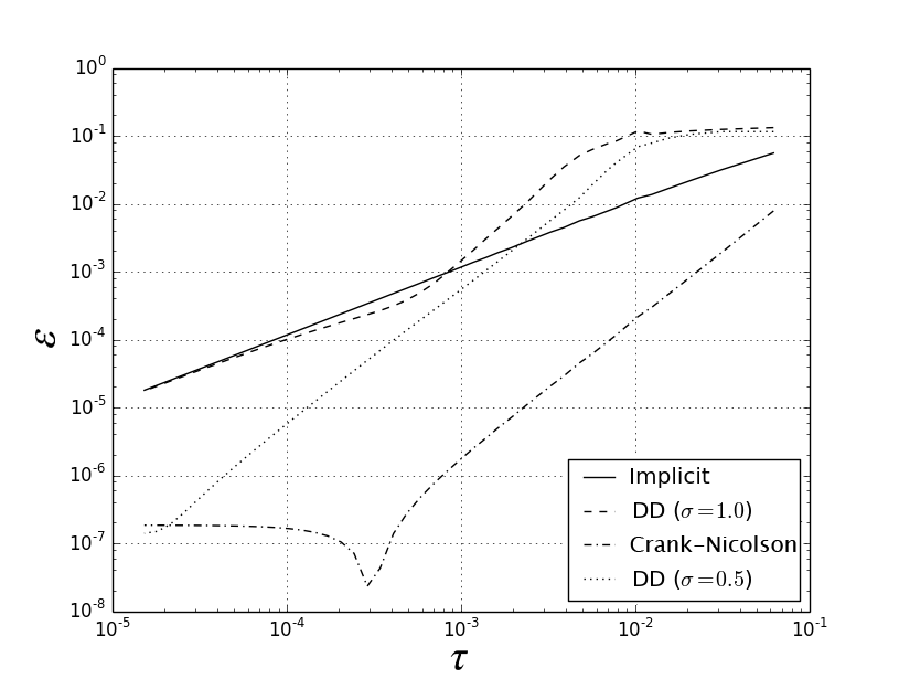
Figure 2: Dependence on time step.

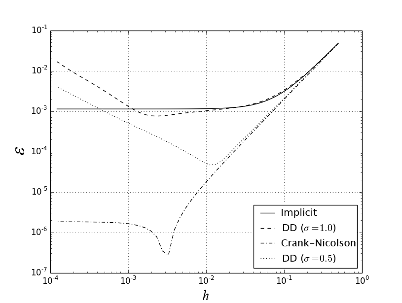
Figure 3: Dependence on mesh size.

The dependence of error on the size of subdomains is shown in Fig. 5. Experiments are conducted for $H=2^{-\gamma/2},\gamma=0,1,...,14$ with $h=2^{-10},\tau=2^{-10},q=h$. Numerical experiments to study the dependence of error on the wight of overlap of subdomains are conducted $q=(2^{\gamma/4+1}-1)h,\ \gamma=4,5,...,36$ with $h=2^{-11},\tau=2^{-9},H=2^{-1}$ and presented in Fig. 5.

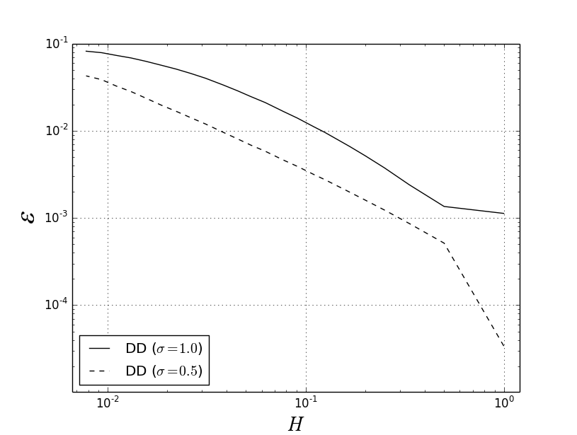
Figure 4: Dependence on size of subdomains.

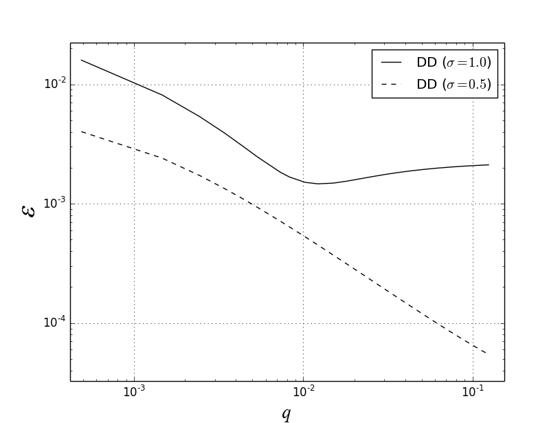
Figure 5: Dependence on width of overlap of subdomains.

References

• Laevsky (1987) Yu. M. Laevsky. Domain decomposition methods for the solution of two-dimensional parabolic equations. In Variational-difference methods in problems of numerical analysis, number 2, pages 112–128, Novosibirsk, 1987. Comp. Cent. Sib. Branch, USSR Acad. Sci. in Russian.
• Marchuk (1990) Gurii I. Marchuk. Splitting and alternating direction methods. In Philip G. Ciarlet and Jacques-Louis Lions, editors, Handbook of Numerical Analysis, Vol. I, pages 197–462. North-Holland, 1990.
• Quarteroni and Valli (1999) Alfio Quarteroni and Alberto Valli. Domain decomposition methods for partial differential equations. Clarendon Press, 1999.
• Samarskii (2001) A. A. Samarskii. The theory of difference schemes. Marcel Dekker, New York, 2001.
• Samarskii et al. (2002) A. A. Samarskii, P. P. Matus, and P. N. Vabishchevich. Difference schemes with operator factors. Kluwer Academic Publishers, 2002.
• Thomée (2006) V. Thomée. Galerkin finite element methods for parabolic problems. Springer Verlag, 2006.
• Toselli and Widlund (2005) Andrea Toselli and Olof Widlund. Domain decomposition methods – algorithms and theory. Springer, 2005.
• Vabishchevich (1989) P. N. Vabishchevich. Difference schemes decompose the computational domain for solving transient problems. Zh. Vychisl. Mat. Mat. Fiz., 29(12):1822–1829, 1989. in Russian.
• Vabishchevich (2014) Petr N. Vabishchevich. Additive Additive Operator-Difference Schemes: Splitting Scheme. De Gruyter, 2014.