A Formulation of the Ring Polymer Molecular Dynamics

Abstract

The exact formulation of the path integral centroid dynamics is extended to include composites of the position and momentum operators. We present the generalized centroid dynamics (GCD), which provides a basis to calculate Kubo-transformed correlation functions by means of classical averages. We define various types of approximate GCD, one of which is equivalent to the ring polymer molecular dynamics (RPMD). The RPMD and another approximate GCD are tested in one-dimensional harmonic system, and it is shown that the RPMD works better in the short time region.

I Introduction

There has been great interest in revealing quantum dynamical aspects of condensed-phase molecular systems such as the liquid hydrogen and liquid helium. The path integral formulation of quantum mechanics FeynmanHibbs is most suited for numerical analysis of complex molecular systems to provide the basis of the path integral Monte Carlo (PIMC) and path integral molecular dynamics (PIMD) Ceperley ; BerneThirumalai ; BerneCiccottiCoker . Most of the static equilibrium properties of finite temperature quantum systems can be computed by means of the PIMC/PIMD techniques. However, it is difficult to apply the PIMC/PIMD directly to compute dynamical properties such as real time quantum correlation functions. This is because the imaginary time path integral formalism is used in the PIMC/PIMD, in which we exploit the isomorphism between the imaginary time path integral representation of the quantum partition function and the classical partition function of a fictitious ring polymer Ceperley ; BerneThirumalai ; BerneCiccottiCoker . In the PIMD simulations, physical quantities are evaluated by time averages of the dynamical variables as in ordinary classical molecular dynamics simulations. However, the time evolution of each bead $q_{j}$ in the ring polymer is just fictitious, and, therefore, we cannot directly evaluate real time-dependent properties by means of the PIMD method.
       A number of quantum dynamics methods to calculate real time quantum correlation functions have been proposed so far Miller ; RabaniReichmanKrilovBerne ; RabaniReichman . In this article, we focus on quantum dynamics methods to calculate Kubo-transformed correlation functions KuboTodaHashitsume $\langle\hat{B}(0)\hat{A}(t)\rangle^{\rm K}_{\beta}$ by means of the PIMD technique. Kubo-transformed correlation functions are important quantities that characterize dynamical effects in quantum mechanical systems, and play a central role in the linear response theory KuboTodaHashitsume . Full quantum correlation functions $\langle\hat{B}(0)\hat{A}(t)\rangle_{\beta}$ can be reproduced from the Kubo-transformed correlation functions using the relation in the frequency space: $\langle\hat{B}\hat{A}\rangle_{\beta}(\omega)=E(\omega)\langle\hat{B}\hat{A}\rangle^{\rm K}_{\beta}(\omega)$, where $E(\omega)$ is a known factor KuboTodaHashitsume .
       Two methods have been proposed so far. One is the centroid molecular dynamics (CMD) CaoVoth and the other is the ring polymer molecular dynamics (RPMD) CraigManolopoulos . The CMD is a classical dynamics of the centroid variables $(q_{c},p_{c})$ on the effective classical potential surface FeynmanKleinert ; GiachettiTognetti . The name “CMD” comes from the fact that the variable $q_{c}$ corresponds to the “centroid” of the ring polymer beads: $q_{0}=(1/P)\sum_{j=1}^{P}q_{j}$. The effective classical potential is a quantum mechanically corrected potential, and can be evaluated by PIMC, PIMD, or other methods. In the most of CMD simulations, however, the “on the fly” integration scheme CaoVoth4 is employed, and, therefore, the CMD is usually implemented by means of the PIMD technique. The CMD can be derived from a more fundamental dynamics, the centroid dynamics (CD), which is defined by the quasi-density operator (QDO) formalism for operators ($\hat{q},\hat{p}$) JangVoth ; JangVoth2 . It has been shown that a correlation function given by the CD is equivalent to the corresponding Kubo-transformed correlation function if the operator $\hat{B}$ is linear in $\hat{q}$ and $\hat{p}$ JangVoth . Therefore, the CD and CMD are not applicable to the case that $\hat{B}$ is nonlinear in them. This is the nonlinear operator problem in the CD. This difficulty can be avoided by considering an improved CD, correlation functions given by which correspond to the higher order Kubo-transformed correlation functions ReichmanRoyJangVoth . However, it is in general difficult to convert those correlation functions to $\langle\hat{B}(0)\hat{A}(t)\rangle_{\beta}$ or $\langle\hat{B}(0)\hat{A}(t)\rangle_{\beta}^{\rm K}$.
       On the other hand, the RPMD is a quite simple method. We just identify the fictitious time evolution of the ring polymer beads in the PIMD as the real time evolution, and then calculate correlation functions $\langle B_{0}(0)A_{0}(t)\rangle_{\beta}^{\rm RPMD}$, where $A_{0}$ and $B_{0}$ are the centroids of position-dependent operators $A(\hat{q})$ and $B(\hat{q})$, respectively CraigManolopoulos . The RPMD has some advantages: we can treat operators nonlinear in $\hat{q}$, and it works well in the short time region to be exact at $t=0$ BraamsManolopoulos . These good properties are ensured by the fact that an identity between a static Kubo-transformed correlation function and the corresponding quantity defined by the path integral, $\langle\hat{B}(0)\hat{A}(0)\rangle_{\beta}^{\rm K}$= $\langle B_{0}(0)A_{0}(0)\rangle_{\beta}^{\rm PI}$, holds for any position-dependent operators. The RPMD looks promising, however, this is just a model and has not been derived from more fundamental theories so far.
       Recently, Hone et al. have pointed out that for the case of $\hat{A}=\hat{B}=\hat{q}$, the RPMD is equivalent to the CMD approximated by the instantaneous force approximation HoneRosskyVoth . Their observation is quite suggestive. This correspondence implies that the RPMD can be formulated as an approximate dynamics of a more fundamental dynamics, just like the CMD is formulated as an approximate CD. However, there is a problem here: The correspondence found by them is limited for the case of $\hat{A}=\hat{B}=\hat{q}$. This is because the CD and CMD have the nonlinear operator problem. Therefore, the QDO formalism should be extended to include operators nonlinear in $\hat{q}$.
       In this article, we develop a new QDO formalism which includes composite operators of $\hat{q}$ and $\hat{p}$. A new CD, the generalized centroid dynamics (GCD), is defined by means of this formalism. We then show that one of the approximate GCD is equivalent to the RPMD.
       This article is organized as follows. In Sec. 2, we introduce the effective classical potential and density for composite operators. In Sec. 3, the QDO formalism is extended to include composite operators, and the GCD is then defined. In Sec. 4, several approximate dynamics are presented and tested in a simple system. Conclusions are given in Sec. 5.

II Effective classical potentials and effective classical densities for composite operators

II.1 Effective classical potentials for composite operators

Consider a quantum system, the Hamiltonian of which is given by

$$\hat{H}=\frac{1}{2m}\hat{p}^{2}+V(\hat{q}).$$ (1)

For simplicity, we use one-dimensional notation in this article, but the multidimensional generalization is straightforward. The density operator of this system is $\hat{\rho}_{\beta}=e^{-\beta\hat{H}}$ and the quantum mechanical partition function is given by the trace of it, $Z_{\beta}={\rm Tr}~{}\hat{\rho}_{\beta}$; here, $\beta=1/(k_{B}T)$ is the inverse temperature. The phase space path integral representation of $Z_{\beta}$ is written as Kleinert

$$Z_{\beta} = \int^{\infty}_{-\infty}\!\!\!dq\int\!\!\!\!\int^{q(\beta\hbar)=q}_{q(0)=q}\!\!\!{\cal D}q{\cal D}p~{}e^{-S[q,p]/\hbar}$$ (2)

$$= \lim_{P\to\infty}\prod_{j=1}^{P}\int\!\!\!\!\int\frac{dq_{j}dp_{j}}{2\pi\hbar}~{}e^{-\beta_{P}H_{P}^{\rm ps}},$$ (3)

where the imaginary time interval $[0,\beta\hbar]$ is discretized into $P$ slices, $q_{j}$ and $p_{j}$ are the position and momentum at the $j$-th time slice, respectively, and $\beta_{P}=\beta/P$. The action $S[q,p]$ is defined by

$$S[q,p]=\int^{\beta\hbar}_{0}\!\!\!d\tau\left(H[q,p]-ip\dot{q}\right),$$ (4)

and the Hamiltonian of $2P$ variables $\{q_{j},p_{j}\}$ is defined by

$$H_{P}^{\rm ps}(\{q_{j},p_{j}\})=\sum_{j=1}^{P}\left.\left[\frac{p^{2}_{j}}{2m}+V(q_{j})-i\frac{p_{j}(q_{j}-q_{j-1})}{\beta_{P}\hbar}\right]\right|_{q_{0}=q_{P}}.$$ (5)

Consider position-dependent Hermitian operators $\{\hat{O}^{(i)}=O^{(i)}(\hat{q})\}~{}(i=1\sim N)$ which are given by operator products of $\hat{q}$ or sums of them. We refer to these operators as composite operators. For each operator $\hat{O}^{(i)}$, there exists a corresponding “centroid” $O_{0}^{(i)}$ in the path integral representation,

$$O_{0}^{(i)}=\frac{1}{\beta\hbar}\int^{\beta\hbar}_{0}\!\!\!d\tau~{}O^{(i)}(q(\tau))=\lim_{P\to\infty}\frac{1}{P}\sum_{j=1}^{P}O^{(i)}(q_{j}).$$ (6)

Inserting $N$ identities $1=\int^{\infty}_{-\infty}dO_{c}^{(i)}\delta(O^{(i)}_{0}-O^{(i)}_{c})$ into the partition function $Z_{\beta}$ (Eq. (2)), we rewrite the partition function as

$$Z_{\beta}=C\prod_{i=1}^{N}\int^{\infty}_{-\infty}\!\!\!dO_{c}^{(i)}~{}e^{-\beta U_{\beta}^{c}(\{O_{c}^{(i)}\})},$$ (7)

where $O_{c}^{(i)}$ is the static centroid variable that corresponds to the centroid $O_{0}^{(i)}$, and $U_{\beta}^{c}(\{O_{c}^{(i)}\})$ is the effective classical potential for composite operators

$$U_{\beta}^{c}(\{O_{c}^{(i)}\})=-\frac{1}{\beta}\log\left[\int^{\infty}_{-\infty}\!\!\!dq\int\!\!\!\!\int^{q(\beta\hbar)=q}_{q(0)=q}\!\!\!{\cal D}q{\cal D}p~{}\prod_{i=1}^{N}\delta(O^{(i)}_{0}-O^{(i)}_{c})e^{-S[q,p]/\hbar}\right]+C.$$ (8)

Here and hereafter, we represent irrelevant constant factors by a symbol $C$. This is the constraint effective potential with many constraints on composite operators, which has been introduced by Fukuda and Kyriakopoulos in the context of quantum field theories FukudaKyriakopoulos .

II.2 Effective classical densities for composite operators

Next, consider Hermitian composite operators $\{\hat{O}^{(i)}={O}^{(i)}(\hat{q},\hat{p})\}~{}(i=1\sim N)$ which are given by operator products of $\hat{q}$, operator products of $\hat{p}$, or sums of them. It should be noted that operators which are products of $\hat{q}$ and $\hat{p}$, such as $(\hat{q}\hat{p}+\hat{p}\hat{q})/2$, are excluded here. The corresponding centroids are given as

$$O_{0}^{(i)}=\frac{1}{\beta\hbar}\int^{\beta\hbar}_{0}\!\!\!d\tau~{}O^{(i)}(q(\tau),p(\tau))=\lim_{P\to\infty}\frac{1}{P}\sum_{j=1}^{P}O^{(i)}(q_{j},p_{j}).$$ (9)

Inserting $N$ identities $1=\int^{\infty}_{-\infty}dO_{c}^{(i)}\delta(O^{(i)}_{0}-O^{(i)}_{c})$ into Eq. (2), we obtain another expression of the quantum partition function

$$Z_{\beta}=C\prod_{i=1}^{N}\int^{\infty}_{-\infty}\!\!\!dO_{c}^{(i)}~{}\rho_{\beta}^{c}(\{O_{c}^{(i)}\}),$$ (10)

where

$$\rho_{\beta}^{c}(\{O_{c}^{(i)}\}) = \frac{1}{C}\int^{\infty}_{-\infty}\!\!\!dq\int\!\!\!\!\int^{q(\beta\hbar)=q}_{q(0)=q}\!\!\!{\cal D}q{\cal D}p~{}\prod_{i=1}^{N}\delta(O^{(i)}_{0}-O^{(i)}_{c})e^{-S[q,p]/\hbar}$$ (11)

$$= e^{-\beta H_{\beta}^{c}(\{O_{c}^{(i)}\})}$$ (12)

is the effective classical density for composite operators, and $H_{\beta}^{c}(\{O_{c}^{(i)}\})$ is the effective classical Hamiltonian. These effective classical quantities enable a classical description of static quantum properties. If we choose $N=2$ and $(\hat{O}^{(1)},\hat{O}^{(2)})=(\hat{q},\hat{p})$, the effective classical Hamiltonian becomes the ordinary one JangVoth

$$H_{\beta}^{c}(q_{c},p_{c})=\frac{p_{c}^{2}}{2m}+V_{\beta}^{c}(q_{c}),$$ (13)

where $V_{\beta}^{c}(q_{c})$ is the ordinary effective classical potential FeynmanKleinert ; GiachettiTognetti .

III Exact centroid dynamics for composite operators

In this section, we extend the QDO formalism JangVoth to include Hermitian composite operators $\{\hat{O}^{(i)}=O^{(i)}(\hat{q},\hat{p})\}$ introduced in the preceding section. Then, we define an exact dynamics of centroid variables and show the exact correspondence between centroid correlation functions and Kubo-transformed correlation functions.

III.1 QDO for composite operators

The canonical density operator for the Hamiltonian (Eq. (1)) can be decomposed as

$$\hat{\rho}_{\beta}=C\prod_{i=1}^{N}\int^{\infty}_{-\infty}\!\!\!dO_{c}^{(i)}~{}\hat{\varphi}^{c}_{\beta}(\{O_{c}^{(i)}\}),$$ (14)

where we introduced an operator

$$\hat{\varphi}_{\beta}^{c}(\{O_{c}^{(i)}\})=\frac{1}{C}\prod_{i=1}^{N}\int^{\infty}_{-\infty}\!\frac{d\eta_{i}}{2\pi}~{}e^{-\beta\hat{H}+i\sum_{i=1}^{N}\eta_{i}(\hat{O}^{(i)}-O_{c}^{(i)})}.$$ (15)

One can see the validity of this decomposition as follows. A position space matrix element of this operator has its phase space path integral representation,

$$\langle q_{b}|\hat{\varphi}_{\beta}^{c}(\{O_{c}^{(i)}\})|q_{a}\rangle=\frac{1}{C}\int\!\!\!\!\int^{q(\beta\hbar)=q_{b}}_{q(0)=q_{a}}\!{\cal D}q{\cal D}p~{}\prod_{i=1}^{N}\int^{\infty}_{-\infty}\!\frac{d\eta_{i}}{2\pi}~{}e^{i\eta_{i}(O^{(i)}_{0}-O^{(i)}_{c})}e^{-S[q,p]/\hbar}.$$ (16)

Taking the trace of this matrix element and using the integral expression of the $\delta$ function, $(2\pi)\delta(O_{0}-O_{c})=\int^{\infty}_{-\infty}\!d\eta~{}e^{i\eta(O_{0}-O{c})}$, we reproduce the effective classical density for composite operators (Eq. (11))

$$\rho^{c}_{\beta}(\{O_{c}^{(i)}\})={\rm Tr}\left[\hat{\varphi}_{\beta}^{c}(\{O_{c}^{(i)}\})\right].$$ (17)

The quantum partition function $Z_{\beta}$ is then reproduced using the expression (Eq. (10)). We define the QDO for composite operators by normalizing the operator $\hat{\varphi}_{\beta}^{c}$,

$$\hat{\delta}_{\beta}^{c}(\{O_{c}^{(i)}\})=\frac{\hat{\varphi}_{\beta}^{c}(\{O_{c}^{(i)}\})}{\rho_{\beta}^{c}(\{O_{c}^{(i)}\})}.$$ (18)

III.2 Generalized centroid dynamics

We define an exact time evolution of the QDO as

$$\hat{\delta}_{\beta}^{c}(t;\{O_{c}^{(i)}\})=e^{-i\hat{H}t/\hbar}~{}\hat{\delta}_{\beta}^{c}(\{O_{c}^{(i)}\})~{}e^{i\hat{H}t/\hbar}.$$ (19)

A dynamical centroid variable $O_{c}^{(i)}(t)$ is then defined by

$$O_{c}^{(i)}(t)={\rm Tr}\left[\hat{\delta}_{\beta}^{c}(t;\{O_{c}^{(i)}\})\hat{O}^{(i)}\right]={\rm Tr}\left[\hat{\delta}_{\beta}^{c}(\{O_{c}^{(i)}\})\hat{O}^{(i)}(t)\right].$$ (20)

This is the GCD, an exact CD for composite operators. In the case of $N=2$ and $(\hat{O}^{(1)},\hat{O}^{(2)})=(\hat{q},\hat{p})$, the GCD is reduced to the original CD proposed by Jang and Voth JangVoth .
       Next, consider a Hermitian operator $\hat{A}=A(\hat{q},\hat{p})$ which is given by operator products of $\hat{q}$, operator products of $\hat{p}$, or sums of them. In terms of the QDO, a classical counterpart to the operator $\hat{A}$ is defined as

$$A_{\beta}^{c}(\{O_{c}^{(i)}\})={\rm Tr}\left[\hat{\delta}_{\beta}^{c}(\{O_{c}^{(i)}\})\hat{A}\right].$$ (21)

This is the effective classical operator for $\hat{A}$, which is a function of static centroid variables $\{O_{c}^{(i)}\}$. The time dependent effective classical operator is given by using time dependent QDO (Eq. (19)),

$$A_{\beta}^{c}(t)=A_{\beta}^{c}(t;\{O_{c}^{(i)}\})={\rm Tr}\left[\hat{\delta}_{\beta}^{c}(t;\{O_{c}^{(i)}\})\hat{A}\right]={\rm Tr}\left[\hat{\delta}_{\beta}^{c}(\{O_{c}^{(i)}\})\hat{A}(t)\right].$$ (22)

If the operator $\hat{A}$ belongs to the operator set $\{\hat{O}^{(i)}\}$ which is chosen to define the QDO, the effective classical operator is equal to the static centroid variable, $A_{\beta}^{c}(\{O_{c}^{(i)}\})=A_{c}$, and the time-dependent effective classical operator equals the dynamical centroid variable $A_{\beta}^{c}(t,\{O_{c}^{(i)}\})=A_{c}(t)$.

III.3 Correlation functions

Consider a couple of Hermitian composite operators, $\hat{A}=A(\hat{q},\hat{p})$ and $\hat{B}=B(\hat{q},\hat{p})$. In terms of the corresponding effective classical operators, we define the centroid correlation function by means of a “classical” ensemble average,

$$\langle B^{c}_{\beta}(0)A^{c}_{\beta}(t)\rangle^{\rm CD}_{\beta} = \frac{1}{Z_{\beta}}C\prod_{i=1}^{N}\int^{\infty}_{-\infty}\!\!\!dO_{c}^{(i)}~{}\rho_{\beta}^{c}(\{O_{c}^{(i)}\})~{}B_{\beta}^{c}A_{\beta}^{c}(t).$$ (23)

If the operator $\hat{B}$ belongs to the operator set $\{\hat{O}^{(i)}\}$, the centroid correlation function (Eq. (23)) is identical to the Kubo-transformed correlation function KuboTodaHashitsume ; JangVoth :

$$\langle B^{c}_{\beta}(0)A^{c}_{\beta}(t)\rangle^{\rm CD}_{\beta} = \langle B_{c}(0)A^{c}_{\beta}(t)\rangle^{\rm CD}_{\beta}$$ (24)

$$= \frac{1}{Z_{\beta}}\int^{\beta}_{0}\!\!\frac{d\lambda}{\beta}~{}{\rm Tr}\left[e^{-(\beta-\lambda)\hat{H}}\hat{B}~{}e^{-\lambda\hat{H}}\hat{A}(t)\right]$$

$$= \langle\hat{B}(0)\hat{A}(t)\rangle^{\rm K}_{\beta},$$

This identity gives us an effective classical way to calculate Kubo-transformed correlation functions. The GCD procedure to calculate $\langle\hat{B}(0)\hat{A}(t)\rangle^{\rm K}_{\beta}$ is summarized as follows: First, we choose an operator set $\{\hat{O}^{(i)}\}$ which includes the operator $\hat{B}$, and calculate the effective classical density $\rho_{\beta}^{c}(\{O_{c}^{(i)}\})$. Second, we compute the GCD trajectories $A_{\beta}^{c}(t)$ by evolving $A_{\beta}^{c}(\{O_{c}^{(i)}\})$, where the initial values of the centroid variables $\{O_{c}^{(i)}\}$ are given by the distribution $\rho_{\beta}^{c}(\{O_{c}^{(i)}\})$. Averaging over the GCD trajectories, we obtain the centroid correlation function (Eq. (23)), which is identical to the Kubo-transformed correlation function.

IV Approximate dynamics: classical CD

Although the GCD identity (Eq. (24)) is exact for the case $\hat{B}\in\{\hat{O}^{i}\}$, the exact computation of the GCD trajectories $A_{\beta}^{c}(t)$ is in general difficult even in simple one-dimensional systems. Therefore, approximations to the GCD are necessary, and we can define various types of approximations. Among them, two approximations, the decoupled centroid approximation and the classical approximation, are especially important for practical applications. The former was introduced by Jang and Voth JangVoth2 , and several effective classical molecular dynamics of centroid variables can be derived via this approximation. A detailed description of such approximate dynamics will be provided elsewhere Horikoshi . On the other hand, the latter, which is presented in this section, reduces the exact CD to various classical dynamics of the path integral beads.

IV.1 Classical approximation

The classical approximation consists of two steps. We first impose an assumption

$$A_{\beta}^{c}(t;\{O_{c}^{(i)}\})\simeq A_{\beta}^{c}(\{O_{c}^{(i)}(t)\}),$$ (25)

which means that the time-dependent effective classical operator is assumed to be a function of dynamical centroid variables $\{O_{c}^{(i)}(t)\}$. Then, we approximate dynamical centroid variables by the corresponding centroids defined by the dynamical path integral beads,

$$O_{c}^{(i)}(t)\simeq O_{0}^{(i)}(t)=\lim_{P\to\infty}\frac{1}{P}\sum_{j=1}^{P}O^{(i)}(q_{j}(t),p_{j}(t)),$$ (26)

where the variables $\{q_{j}(t),p_{j}(t)\}$ are assumed to evolve in a classical fashion. This is the classical centroid dynamics (CCD), an approximate dynamics of the GCD. Various types of classical time evolutions of the path integral beads can be introduced to define various types of CCD. In the CCD, the centroid correlation functions (Eq. (23)) are evaluated by means of the molecular dynamics techniques; if the dynamics is ergodic, ensemble averages can be obtained by taking time averages of trajectories given by solving a set of classical equations of motion. In the following subsections, we present several variations of the CCD and resulting correlation functions.
       Here, we give some comments on symmetries of Kubo-transformed correlation functions. In the case that $(\hat{A},\hat{B})=(A(\hat{q}),B(\hat{q}))$, the Kubo-transformed correlation function has the same symmetries as the corresponding correlation functions defined in classical statistical mechanics CraigManolopoulos . Therefore, in this case, the centroid correlation function (Eq. (23)) might be calculated by means of the classical molecular dynamics techniques. However, in case of $(\hat{A},\hat{B})=(A(\hat{p}),B(\hat{p}))$, the time-reversal symmetry of the Kubo-transformed correlation function holds only if $\hat{A}=\hat{B}$ or the potential $V(\hat{q})$ is parity symmetric. Furthermore, in the case that $(\hat{A},\hat{B})=(A(\hat{q}),B(\hat{p}))$ or $(A(\hat{p}),B(\hat{q}))$, the time-reversal symmetry is in general broken. These facts suggest that in those cases, molecular dynamical calculations of centroid correlation functions do not work very much.

IV.2 Phase space CCD

We first consider a classical dynamics where dynamical variables $\{q_{j}(t),p_{j}(t)\}$ evolve according to Hamilton’s equations of motion with the Hamiltonian $H_{P}^{\rm ps}$ (Eq. (5)),

$$\frac{d}{dt}q_{j}(t) = \frac{\partial H_{P}^{\rm ps}}{\partial p_{j}},$$ (27)

$$\frac{d}{dt}p_{j}(t) = -\frac{\partial H_{P}^{\rm ps}}{\partial q_{j}}.$$ (28)

If the system is ergodic, the correlation function can be evaluated as

$$\langle B^{c}_{\beta}(0)A^{c}_{\beta}(t)\rangle^{\rm CD}_{\beta}\simeq\lim_{P\to\infty}\frac{1}{Z_{\beta}}\prod_{j=1}^{P}\int\!\!\!\!\int\frac{dq_{j}dp_{j}}{2\pi\hbar}~{}e^{-\beta_{P}H_{P}^{\rm ps}}B^{c}_{\beta}(\{O^{(i)}_{0}(0)\})A^{c}_{\beta}(\{O^{(i)}_{0}(t)\}).$$ (29)

We refer to this dynamics as the phase space classical centroid dynamics (PS-CCD) because the classical time evolution is governed by the Hamiltonian $H_{P}^{\rm ps}$ in the phase space path integral representation.

It should be noted here that the PS-CCD is not suited for practical calculations because the imaginary term in the Hamiltonian, $-ip_{j}(q_{j}-q_{j-1})/(\beta_{P}\hbar)$, makes the dynamics ill-defined.

IV.3 Fictitious momenta and masses: summary of the PIMD

The PS-CCD has the problem originating in the fact that the Hamiltonian $H_{P}^{\rm ps}$ is complex. On the other hand, in ordinary PIMD simulations, we never encounter this kind of difficulty because we use the configuration space path integral representation of the quantum partition function,

$$Z_{\beta} = \lim_{P\to\infty}\prod_{j=1}^{P}\sqrt{\frac{m}{2\pi\beta_{P}\hbar^{2}}}\int dq_{j}~{}e^{-\beta_{P}V_{P}^{\rm cs}}.$$ (30)

This expression can be derived from the phase space path integral expression (Eq. (3)) by integrating out the momentum variables $\{p_{j}\}$. The potential $V_{P}^{\rm cs}$ is given by

$$V_{P}^{\rm cs}(\{q_{j}\})=\sum_{j=1}^{P}\left.\left[~{}\frac{1}{2}k_{P}(q_{j}-q_{j-1})^{2}+V(q_{j})~{}\right]\right|_{q_{0}=q_{P}},$$ (31)

where $k_{P}=m/(\beta_{P}^{2}\hbar^{2})$. Inserting $P$ identities $1=\sqrt{\beta_{P}/(2\pi\tilde{m}_{j})}\int^{\infty}_{-\infty}d\tilde{p}_{j}~{}e^{-\beta_{P}\tilde{p}_{j}^{2}/(2\tilde{m}_{j})}$ into $Z_{\beta}$ (Eq. (30)), we obtain

$$Z_{\beta}=\lim_{P\to\infty}\prod_{j=1}^{P}\sqrt{\frac{m}{\tilde{m}_{j}}}\int\!\!\!\!\int\frac{dq_{j}d\tilde{p}_{j}}{2\pi\hbar}~{}e^{-\beta_{P}H_{P}^{\rm cs}},$$ (32)

where the Hamiltonian is given by

$$H_{P}^{\rm cs}=\sum_{j=1}^{P}\frac{\tilde{p}_{j}^{2}}{2\tilde{m}_{j}}+V_{P}^{\rm cs}.$$ (33)

New momenta $\{\tilde{p}_{j}\}$ and masses $\{\tilde{m}_{j}\}$ are introduced as fictitious momenta and masses, respectively. This is the partition function used in the configuration space PIMD simulations BerneThirumalai ; BerneCiccottiCoker .
       In most of PIMD simulations, we often use a transformation from the bead variables $\{q_{j}\}$ to normal modes $\{x_{n}\}$,

$$x_{n}=\sum^{P}_{j=1}U_{nj}q_{j},$$ (34)

where $U$ is a unitary matrix. If we transform the variables $\{q_{j}\}$ in Eq. (30) using an orthogonal matrix

$$U_{nj}=\frac{1}{\sqrt{P}}\left(\cos\frac{2\pi nj}{P}-\sin\frac{2\pi nj}{P}\right),$$ (35)

and insert $P$ identities $1=\sqrt{\beta_{P}/(2\pi\tilde{m}_{n})}\int^{\infty}_{-\infty}d\tilde{p}_{n}~{}e^{-\beta_{P}\tilde{p}_{n}^{2}/(2\tilde{m}_{n})}$ into Eq. (30), we obtain another expression of the quantum partition function,

$$Z_{\beta}=\lim_{P\to\infty}\prod_{n=1}^{P}\sqrt{\frac{m}{\tilde{m}_{n}}}\int\!\!\!\!\int\frac{dx_{n}d\tilde{p}_{n}}{2\pi\hbar}~{}e^{-\beta_{P}H_{P}^{\rm NM}},$$ (36)

where the Hamiltonian is given by

$$H_{P}^{\rm NM}(\{x_{n},\tilde{p}_{n}\})=\sum_{n=1}^{P}\left[\frac{\tilde{p}_{n}^{2}}{2\tilde{m}_{n}}+\left(2k_{P}\sin^{2}\frac{\pi n}{P}\right)x_{n}^{2}+\tilde{V}(\{x_{n}\})\right].$$ (37)

This kind of expression of the partition function is used in the normal mode PIMD simulations BerneThirumalai ; BerneCiccottiCoker .

IV.4 Configuration space CCD

Here we introduce another type of CCD, the configuration space classical centroid dynamics (CS-CCD). There are two expressions of the CS-CCD. One is a classical dynamics governed by Hamilton’s equations of motion for the bead variables $\{q_{j}(t),\tilde{p}_{j}(t)\}$,

$$\frac{d}{dt}q_{j}(t) = \frac{\partial H_{P}^{\rm cs}}{\partial\tilde{p}_{j}},$$ (38)

$$\frac{d}{dt}\tilde{p}_{j}(t) = -\frac{\partial H_{P}^{\rm cs}}{\partial q_{j}},$$ (39)

where $H_{P}^{\rm cs}$ is the Hamiltonian (Eq. (33)) used in the configuration space PIMD. If the dynamics is ergodic, the correlation function is given by

$$\langle B^{c}_{\beta}(0)A^{c}_{\beta}(t)\rangle^{\rm CD}_{\beta}\simeq\lim_{P\to\infty}\frac{1}{Z_{\beta}}\prod_{j=1}^{P}\sqrt{\frac{m}{\tilde{m}_{j}}}\int\!\!\!\!\int\frac{dq_{j}d\tilde{p}_{j}}{2\pi\hbar}~{}e^{-\beta_{P}H_{P}^{\rm cs}}B^{c}_{\beta}(\{O^{(i)}_{0}(0)\})A^{c}_{\beta}(\{O^{(i)}_{0}(t)\}).$$ (40)

We refer to this dynamics as the ring polymer CS-CCD because the variables $\{q_{j}(t)\}$ form a ring polymer where the nearest neighbors are connected with the spring constant $k_{P}$.
       The other expression of the CS-CCD is a classical dynamics of the normal mode variables $\{x_{n}(t),\tilde{p}_{n}(t)\}$. This is the normal mode CS-CCD, which is governed by Hamilton’s equations of motion with the Hamiltonian $H_{P}^{\rm NM}$ (Eq. (37)),

$$\frac{d}{dt}x_{n}(t) = \frac{\partial H_{P}^{\rm NM}}{\partial\tilde{p}_{n}},$$ (41)

$$\frac{d}{dt}\tilde{p}_{n}(t) = -\frac{\partial H_{P}^{\rm NM}}{\partial x_{n}}.$$ (42)

If the ergodicity of the dynamics is satisfied, the correlation function is given by

$$\langle B^{c}_{\beta}(0)A^{c}_{\beta}(t)\rangle^{\rm CD}_{\beta}\simeq\lim_{P\to\infty}\frac{1}{Z_{\beta}}\prod_{n=1}^{P}\sqrt{\frac{m}{\tilde{m}_{n}}}\int\!\!\!\!\int\frac{dx_{n}d\tilde{p}_{n}}{2\pi\hbar}~{}e^{-\beta_{P}H_{P}^{\rm NM}}B^{c}_{\beta}(\{O^{(i)}_{0}(0)\})A^{c}_{\beta}(\{O^{(i)}_{0}(t)\}).$$ (43)

Here, we give two comments on the CS-CCD: (1) In general systems, the CS-CCD is exact only for the calculation of the static correlation functions $\langle B^{c}_{\beta}(0)A^{c}_{\beta}(0)\rangle$ for position-dependent operators $(A(\hat{q}),B(\hat{q}))$. In the case of $t\neq 0$ or momentum-dependent operators, the fictitious momenta $\{\tilde{p}_{j}\}$ (or $\{\tilde{p}_{n}\}$) enlarge the gap between the CS-CCD correlation function and the Kubo-transformed correlation function. Therefore, the validity of the CS-CCD expressions (Eqs. (40) or (43)) should be checked depending on the situation. (2) The choice of the fictitious masses is crucial. In the normal mode CS-CCD, if the fictitious mass of $P$-th normal mode is chosen as $\tilde{m}_{P}=m$, then the CS-CCD gives the exact correlation function $\langle B^{c}_{\beta}(0)A^{c}_{\beta}(0)\rangle$ for $\hat{A}=\hat{B}=\hat{p}\in\{\hat{O}^{(i)}\}$. This is because the choice $\tilde{m}_{P}=m$ connects the fictitious momentum $\tilde{p}_{P}$ with the physical momentum centroid $p_{0}$ via the centroid expression of the density (Eqs. (12) and (13)). In the ring polymer CS-CCD, this condition can be satisfied by setting $\{\tilde{m}_{j}=m\}$, i.e. setting all fictitious masses equal to the physical mass.

IV.5 Ring polymer molecular dynamics

Finally, we present a special case of the ring polymer CS-CCD. If the operators $(\hat{A},\hat{B})$ belong to the operator set $\{\hat{O}^{(i)}\}$, and all fictitious masses are chosen to be the physical mass, $\{\tilde{m}_{j}=m\}$, the ring polymer CS-CCD correlation function (Eq. (40)) becomes

$$\langle B^{c}_{\beta}(0)A^{c}_{\beta}(t)\rangle^{\rm CD}_{\beta}\simeq\lim_{P\to\infty}\frac{1}{Z_{\beta}}\prod_{j=1}^{P}\int\!\!\!\!\int\frac{dq_{j}d\tilde{p}_{j}}{2\pi\hbar}~{}e^{-\beta_{P}H_{P}^{\rm cs}}B_{0}(0)A_{0}(t).$$ (44)

This dynamics is equivalent to the RPMD proposed by Craig and Manolopoulos CraigManolopoulos . As we mentioned in the preceding subsection, the RPMD reproduces the exact correlation functions at $t=0$ for $(\hat{A},\hat{B})=(A(\hat{q}),B(\hat{q}))$ or $(\hat{p},\hat{p})$. Recently, it has been shown that for the calculations of $\langle\hat{q}(0)\hat{q}(t)\rangle^{\rm K}_{\beta}$ and $\langle\hat{p}(0)\hat{p}(t)\rangle^{\rm K}_{\beta}$, the RPMD is correct up to $O(t^{6})$ and $O(t^{4})$, respectively BraamsManolopoulos .

IV.6 Simple example: a harmonic system

Here, we consider the case $\hat{A}=\hat{B}=\hat{q}^{2}\in\{\hat{O}^{(i)}\}$, and show the results of two types of approximate CD: the RPMD and the normal mode CS-CCD. We consider a simple system with a harmonic potential $V(\hat{q})=(m\omega^{2}/2)\hat{q}^{2}$. In this system, the exact Kubo-transformed “position squared” autocorrelation function is given by

$$\langle\hat{q}^{2}(0)\hat{q}^{2}(t)\rangle_{\beta}^{\rm K} = \frac{\hbar^{2}}{4m^{2}\omega^{2}}\left[\frac{2}{\beta\hbar\omega}\coth\frac{\beta\hbar\omega}{2}\cos 2\omega t+2\coth^{2}\frac{\beta\hbar\omega}{2}-1\right].$$ (45)

The corresponding RPMD correlation function is calculated as

$$\langle\hat{q}^{2}(0)\hat{q}^{2}(t)\rangle_{\beta}^{\rm RPMD} = \lim_{P\to\infty}\frac{1}{\beta^{2}m^{2}}\left[\sum_{n=1}^{P}\frac{1}{\omega_{n}^{4}}(\cos 2\omega_{n}t+1)+\sum_{n=1}^{P}\sum_{l=1}^{P}\frac{1}{\omega_{n}^{2}\omega_{l}^{2}}\right],$$ (46)

where $\omega_{n}=\sqrt{\omega^{2}+(4k_{P}/m)\sin^{2}(\pi n/P)}$. The corresponding normal mode CS-CCD correlation function is also obtained as

$$\langle\hat{q}^{2}(0)\hat{q}^{2}(t)\rangle_{\beta}^{\rm NM} = \lim_{P\to\infty}\frac{1}{\beta^{2}m^{2}}\left[\sum_{n=1}^{P}\frac{1}{\omega_{n}^{4}}(\cos 2\Omega_{n}t+1)+\sum_{n=1}^{P}\sum_{l=1}^{P}\frac{1}{\omega_{n}^{2}\omega_{l}^{2}}\right],$$ (47)

where $\Omega_{n}=\omega_{n}\sqrt{m/\tilde{m}_{n}}$.
       Figure 1 shows the plot of the three correlation functions, Eqs. (45)–(47), at two different temperatures with the parameters $\hbar=k_{B}=m=\omega=1$. We set the number of beads $P$ as $1000$, which is so large as to make the results converged sufficiently. The fictitious masses of the normal modes are chosen as $\{\tilde{m}_{n}=m+(4m/\beta_{P}^{2}\hbar^{2}\omega^{2})\sin^{2}(\pi n/P)\}$. This choice makes each frequency $2\Omega_{n}$ equal to $2\omega$. At the higher temperature $\beta=1$ (Fig. 1 (a)), the RPMD correlation function and the normal mode CS-CCD correlation function are almost identical, and they coincide with the exact Kubo-transformed correlation function at $t=0$. However, as the time $t$ increases, they slightly deviate from the exact correlation function. These deviations become more significant at the lower temperature $\beta=10$ (Fig. 1 (b)). As is observed clearly in Fig. 1 (b), the RPMD correlation function damps with time. This is because the mode summation $\sum_{n=1}^{P}$ causes a dephasing effect. The lower the temperature falls, the more modes with different frequencies are relevant in the summation $\sum_{n=1}^{P}$. Therefore, the dephasing effect becomes stronger at lower temperature. On the other hand, the normal mode CS-CCD correlation function is free from such a dephasing effect, thanks to the special choice of fictitious masses $\{\tilde{m}_{n}\}$. However, as one can also see in Fig. 1 (b), the short time behavior of $\langle\hat{q}^{2}(0)\hat{q}^{2}(t)\rangle_{\beta}^{\rm NM}$ is worse than $\langle\hat{q}^{2}(0)\hat{q}^{2}(t)\rangle_{\beta}^{\rm RPMD}$. This is because the mass choice adopted in the RPMD, $\{\tilde{m}_{j}=m\}$, is the optimized one to reproduce the short time behaviors of exact Kubo-transformed correlation functions BraamsManolopoulos . These observations in the simple harmonic system show the importance of the mass choice. If you focus on the short time behaviors of correlation functions, you should choose $\{\tilde{m}_{j}=m\}$. On the other hand, if you respect the dynamical quantum effects such as coherent oscillations of correlation functions, another choice might be better.

V Concluding remarks

In this work, we have developed an exact CD for composite operators of $\hat{q}$ and $\hat{p}$, the GCD, which gives an exact identity between a centroid correlation function and a Kubo-transformed correlation function (Eq. (24)). We have then proposed the classical approximation and the corresponding approximate GCD, the CCD (Eqs. (25) and (26)). Introducing several types of classical time evolutions, we have defined several types of CCD, the PS-CCD (Eqs. (27) and (28)), the ring polymer CS-CCD (Eqs. (38) and (39)), and the normal mode CS-CCD (Eqs. (41) and (42)). If we consider operators $\hat{A}$ and $\hat{B}$ which belong to the operator set $\{\hat{O}^{(i)}\}$, and set the fictitious masses equal to the physical mass, $\{\tilde{m}_{j}=m\}$, the ring polymer CS-CCD becomes equivalent to the RPMD proposed by Craig and Manolopoulos (Eq. (44)) CraigManolopoulos . A schematic diagram of various approximate dynamics is given in Fig. 2. The results of simple calculations in a harmonic system have shown that the choice of fictitious masses is crucial in CS-CCD calculations. The RPMD might be the best CS-CCD method to calculate correlation functions in the short time region.
       We have shown that the RPMD can be formulated as an approximate GCD. However, the classical approximation employed there is rather crude. The physical meaning of the approximation should be clarified, and systematic schemes to improve the approximation should be developed. Recently, a relationship between the RPMD and the semiclassical instanton theory has been discussed in the deep tunneling regime, and it has been shown that the RPMD can be systematically improved in that regime RichardsonAlthorpe .
       Finally, we briefly mention another approximation scheme. Applying the decoupled centroid approximation to the GCD, we obtain the generalized centroid molecular dynamics (GCMD) Horikoshi . In the case of $N=2$ and $(\hat{O}^{(1)},\hat{O}^{(2)})=(\hat{q},\hat{p})$, the GCMD is reduced to the CMD proposed by Cao and Voth CaoVoth . The relations between these methods are summarized in Fig. 2. The GCMD is a dynamics of centroid variables $\{O_{c}^{(i)}(t)\}$ rather than centroids $\{O_{0}^{(i)}(t)\}$ defined by the summation of the path integral beads. Therefore, the GCMD correlation functions are expected to be free from the summation-induced dephasing effect seen in the RPMD correlation functions (Fig. 1). However, in general, it is not so easy to formulate the GCMD and to implement it for practical calculations. This is because the GCMD is a non-Hamiltonian dynamics which should be formulated in an extended phase space spanned by canonical multiplets Horikoshi . A proper formulation of the GCMD might be given by a generalized Hamiltonian dynamics proposed by Nambu Nambu .

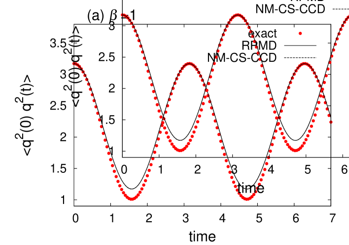
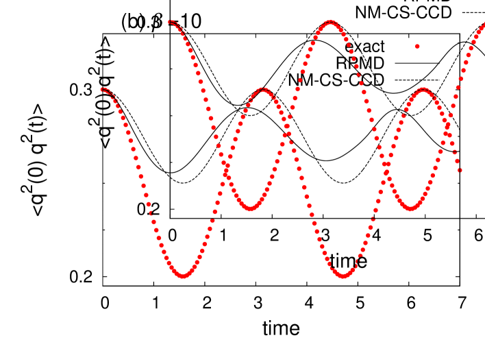
Figure 1: The plot of the exact Kubo-transformed correlation function (Eq. (45)), the RPMD correlation function (Eq. (46)), and the normal mode CS-CCD correlation function (Eq. (47)) for the quantum harmonic oscillator: (a) in the higher temperature regime ($\beta=1$) and (b) in the lower temperature regime ($\beta=10$).

Figure 2: Schematic diagram for the GCD and its approximate dynamics. The first up-down arrow represents the equivalence between Kubo-transformed correlation functions and centroid correlation functions given by the GCD (Eq. (24)). The left-hand route to the RPMD is obtained via the classical approximation. Detailed descriptions on the right-hand route to the CMD have not been presented in this article Horikoshi .

References

• (1) R. P. Feynman and A. R. Hibbs, Quantum Mechanics and Path integrals, McGraw-Hill, New York, 1965.
• (2) D. M. Ceperley, Path integrals in the theory of condensed helium, Rev. Mod. Phys. 67 (1995), pp. 279–355.
• (3) B. J. Berne and D. Thirumalai, On the Simulation of Quantum Systems: Path Integral Methods, Annu. Rev. Phys. Chem. 37 (1986), pp. 401–424.
• (4) B. J. Berne, G. Ciccotti, and D. F. Coker (ed.), Classical and Quantum Dynamics in Condensed Phase Simulations, World Scientific, Singapore, 1998.
• (5) W. H. Miller, Chemical Theory and Computation Special Feature: Quantum dynamics of complex molecular systems, Proc. Natl. Acad. Sci. U.S.A. 102 (2005), pp. 6660–6664.
• (6) E. Rabani, D. R. Reichman, G. Krilov, and B. J. Berne, The calculation of transport properties in quantum liquids using the maximum entropy numerical analytic continuation method: Application to liquid para-hydrogen, Proc. Natl. Acad. Sci. U.S.A. 99 (2002), pp. 1129–1133.
• (7) E. Rabani and D. R. Reichman, QUANTUM MODE-COUPLING THEORY: Formulation and Applications to Normal and Supercooled Quantum Liquids, Annu. Rev. Phys. Chem. 56 (2005), pp. 157–185.
• (8) R. Kubo, N. Toda, and N. Hashitsume, Statistical Physics II, Springer, Berlin, 1985.
• (9) J. Cao and G. A. Voth, The formulation of quantum statistical mechanics based on the Feynman path centroid density. II. Dynamical properties, J. Chem. Phys. 100 (1994), pp. 5106–5117.
• (10) I. R. Craig and D. E. Manolopoulos, Quantum statistics and classical mechanics: Real time correlation functions from ring polymer molecular dynamics, J. Chem. Phys. 121 (2004), pp. 3368–3373.
• (11) R. P. Feynman and H. Kleinert, Effective classical partition functions, Phys. Rev. A 34 (1986), pp. 5080–5084.
• (12) R. Giachetti and V. Tognetti, Variational Approach to Quantum Statistical Mechanics of Nonlinear Systems with Application to Sine-Gordon Chains, Phys. Rev. Lett. 55 (1985), pp. 912–915.
• (13) J. Cao and G. A. Voth, The formulation of quantum statistical mechanics based on the Feynman path centroid density. IV. Algorithms for centroid molecular dynamics, J. Chem. Phys. 101 (1994), pp. 6168–6183.
• (14) S. Jang and G. A. Voth, Path integral centroid variables and the formulation of their exact real time dynamics, J. Chem. Phys. 111 (1999), pp. 2357–2370.
• (15) S. Jang and G. A. Voth, A derivation of centroid molecular dynamics and other approximate time evolution methods for path integral centroid variables, J. Chem. Phys. 111 (1999), pp. 2371–2384.
• (16) D. R. Reichman, P. -N. Roy, S. Jang, and G. A. Voth, A Feynman path centroid dynamics approach for the computation of time correlation functions involving nonlinear operators, J. Chem. Phys. 113 (2000), pp. 919–929.
• (17) B. J. Braams and D. E. Manolopoulos, On the short-time limit of ring polymer molecular dynamics, J. Chem. Phys. 125 (2006), pp. 124105 1–9.
• (18) T. D. Hone, P. J. Rossky, and G. A. Voth, A comparative study of imaginary time path integral based methods for quantum dynamics, J. Chem. Phys. 124 (2006), pp. 154103 1–9.
• (19) H. Kleinert, Path Integrals in Quantum Mechanics, Statistics, Polymer Physics, and Financial Markets, World Scientific, Singapore, 2004.
• (20) R. Fukuda and E. Kyriakopoulos, Derivation of the effective potential, Nucl. Phys. B 85 (1975), pp. 354–364.
• (21) A. Horikoshi, in preparation.
• (22) J. O. Richardson and S. C. Althorpe, Ring-polymer molecular dynamics rate-theory in the deep-tunneling regime: Connection with semiclassical instanton theory, J. Chem. Phys. 131 (2009), pp. 214106 1–12.
• (23) Y. Nambu, Generalized Hamiltonian Dynamics, Phys. Rev. D 7 (1973), pp. 2405–2412.
Refer to caption
Refer to caption