Using CMOS Sensors in a Cellphone for Gamma Detection and Classification

Abstract

The CMOS camera found in many cellphones is sensitive to ionized electrons. Gamma rays penetrate into the phone and produce ionized electrons that are then detected by the camera. Thermal noise and other noise needs to be removed on the phone, which requires an algorithm that has relatively low memory and computational requirements. The continuous high-delta algorithm described fits those requirements. Only a small fraction of the energy of even the electron is deposited in the camera sensor, so direct methods of measuring the energy cannot be used. The fraction of groups of lit up pixels that are lines is correlated with the energy of the gamma rays. This correlation under certain conditions allows limited low resolution energy resolution to be performed.

1 Introduction

Charge-coupled device (CCD) detectors have been used in X-ray detection and spectroscopy for over a decade. Complementary metal-oxide-semiconductor (CMOS) sensors have recently begun to be used similarly. Since a cellphone contains a CMOS sensor and computational ability, the CellRad project (Derr et al., 2012) was created to characterize the cellphone’s ability as a gamma radiation sensor. This project tested both the ability of the cellphone to operate as a simple dose rate sensor, and—when using additional processing on the server side—to do low resolution spectroscopy. For these tests, the lens is covered with electrical tape to block the light, but otherwise the only modification to the cellphone is the addition of software.

2 Review of Literature

CCD have been used for X-ray detection and spectroscopy (Knoll, 2000; Holland, 1996). The CCDs are typically cooled to reduce the generation of dark current (MacDonald et al., 1997). The amplification of CCD (which is used to determine the energy in electron volts deposited per pixel) can be simply measured if access to the raw pixel values are available (Janesick, 2001; Cogliati, 2010). CMOS have not typically been used because of lower signal-to-noise ratio and lower dynamic range. However, lower cost and power are two advantages to using CMOS, and while CMOS technology is improving and there are mitigations for reducing the noise (Kim et al., 2006). For X-ray spectroscopy, for many events, all the energy is deposited in a single pixel or a group of pixels, and then this energy can be directly measured (Ishiwatari et al., 2006).

Using the camera in a cellphone to detect radiation has been proposed (mike449, 2008), and several applications are now commercially available (Quick, 2011; Gabel, 2012; Drukier et al., 2011).

3 Physics Overview

Radioactive sources produce ionizing radiation every time a single atom decays into another atom. This ionizing radiation can come in several forms including beta (which are high-energy electrons), alpha (which is a helium nucleus), and gamma (which are high energy photons). The beta and alpha particles will be stopped fairly quickly when they travel through material, but the gamma photons can travel long distances before being absorbed.

Different isotopes produce different types of ionizing radiation and different energies of the radiation. For example ¹³⁷Cs produces 662 keV photons, but ⁶⁰Co produces 1173 and 1332 keV photons. Ordinary light is non-ionizing and has much lower energies that are in the eV range. For example the photons for red light have about 1.77 eV of energy, and the range goes up to 3.10 eV for violet light photons.

The photons interact in a variety of ways with the material. The most important for CellRad are the photoelectric effect and Compton scattering. The photoelectric effect is dominate at lower energies. For example, almost all visible light photons that a material absorbs will be absorbed by the photoelectric effect. In the photoelectric effect, the incoming photon’s energy is completely absorbed, and the energy is transferred to an electron that is ionized (that is, stripped off of an atom).

Compton scattering is dominate at intermediate energies around 1 MeV. In Compton scattering, the incoming photon transfers some of its energy to the electron that it ionizes. This results in the ionized electron having only part of the energy of the photon, so the energy will vary (Mayo, 1998).

The relation between the angle of the electron, the energy of the electron, and the energy of incoming photon in Compton scattering is:

$$\frac{KE_{e}(E_{\gamma}+m_{e}c^{2})}{E_{\gamma}\sqrt{KE_{e}(2m_{e}c^{2}+KE_{e})}}=cos\phi_{e}$$ (1)

where $KE_{e}$ is the energy of the electron, $E_{\gamma}$ is the energy of the photon, $\phi_{e}$ is the angle the electron scatters and $2m_{e}c^{2}$ is approximately 511 keV. Figure 1 shows two different distributions of this equation.

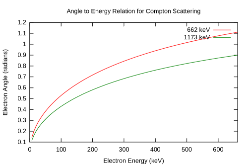
Figure 1: Compton electron angle-to-energy relations for 662 keV and 1173 keV photons

The ionized electrons may have energy that is much higher than the energy required to ionize a single electron. In that case, the high energy electrons will ionize secondary electrons, which will continue until the energy has been lowered significantly. A 20 keV electron might ionize 10,000 secondary electrons. Electrons with high enough energies will leave trails of ionization as they travel through the material. The higher the energy, the less energy that an electron will typically leave in a given distance (which is related to stopping power).

4 Silicon Surface Barrier Experiments

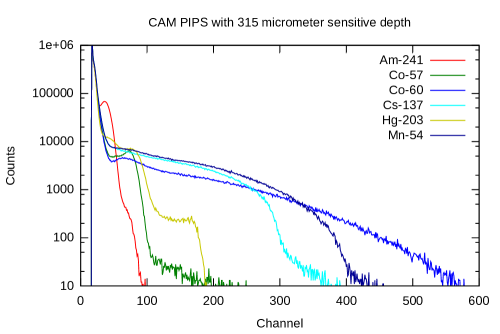
Figure 2: 315 micron ($\mu$m) sensitive depth spectrum

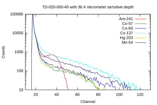
Figure 3: 36.4 micron ($\mu$m) sensitive depth spectrum

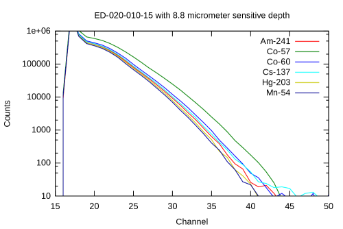
Figure 4: 8.8 micron ($\mu$m) sensitive depth spectrum

In order to help understand the physics of electrons in silicon, several experiments were run using silicon surface barrier detectors. The depth of the sensitive region is not a number that manufacturers of CMOS cameras provide, but review of the literature gives an estimate that the thickness is in the range of 10 microns to 0.1 microns (Janesick, 2001; Yadid-Pecht and Etienne-Cummings, 2004). Silicon surface barrier detectors were used as a proxy for a cellphone camera. Three detectors were used. The largest was a CAM Passivated Implanted Planar Silicon (PIPS) detector produced by Canberra Industries, Inc which had a sensitive depth (for beta particles) of 315 microns. The two smaller surface barrier detectors were produced by Ortec Advanced Measurement Technology, Inc. They are both D-series planar totally depleted silicon surface barrier detectors. These detectors were chosen because they are very thin, only 36.4 and 8.8 microns respectively. The smaller detector is similar in thickness to a pixel in a digital camera. For all semiconductor radiation detector measurements, an SMB connector attached the detector signal cable to an Ortec model 142B pre-amplifier, then on to an Ortec model 572 amplifier and an Ortec model 927 Aspec MCA. The voltage was supplied by a Canberra model 3102D HV supply.

Even with the thickest detector used in these experiments, energy spectrum determination is difficult, because of the size of the detector only part of the energy of the gamma ray remains in the detector. Compton edges can be seen in Figure 2. The Compton edge for ²⁴¹Am at 11 keV can be seen distinctly. However, as the energy of the gamma ray increases the Compton edges become smeared out, and the ones at 963 keV and 1117 keV for ⁶⁰Co are not clear. Essentially, the higher the energy of the electron, the higher the probability that it will exit the detector with significant energy, instead of depositing the full energy of the Compton scattered electron. When the thinner 36.4 micron detector is used, only the ²⁴¹Am retains significant structure in Figure 3 (Note that the number of channels is decreased in the graph because less energy was deposited). With the thinnest detector, there is very little spectrum information remaining in Figure 4 and much smaller amounts of energy deposited. From this data, direct measurement of the energy spectrum is expected to be difficult to impossible with a cellphone camera that has a sensitive region with a thickness around 10 microns or less.

5 CMOS Overview

CCD and CMOS cameras work with visible light by using the photoelectric effect. Photons with energies between 1.1 eV to 3.1 eV ionize one electron creating a single electron-hole pair (Janesick, 2001). This electron is then captured in the depletion region of a photodiode or capacitor. An electric field is used to separate the electron from the hole in the depletion region, otherwise they might recombine. After the collection time has passed, the total number of electrons is measured and this measurement is used to determine the brightness for that particular pixel. For CCD cameras, the electrons are transferred to a common amplifier and analog to digital converter. For CMOS cameras every pixel has at least one active transistor, so part of the amplification and measurement occurs at each pixel (Yadid-Pecht and Etienne-Cummings, 2004). Besides photons causing ionized electrons, electrons can also be produced by leaky circuits and by heat. These electrons result in signal even when there is no light. These effects tend to be similar from image to image with the same sensor; when the same sensor is the same temperature, the defects are even more similar from picture to picture.

For creating colored images, the pixels have different filters put between the lens and the pixel, which only let a specific color through. For example, the first row of pixels might be Red Green R G R G …and the second row would be Green Blue G B G B …(Holst, 1998) These individual colors are combined together to create the full image. Note that the full image that is returned usually interpolates the colors to find an individual pixel, so it includes data from multiple pixels (so the first pixel would get most of its red data from the physical R, but the G would be interpolated from the nearby physical pixels). For detecting radiation, the color processing makes determining actual energy deposited on the physical pixels very difficult. For radiation detection, the camera is covered so there is no signal from light. The images also are often compressed, which for “lossy” formats such as JPEG, results in compression artifacts.

The gamma rays continually produce ionized electrons. When there is an electric field present, the electrons will be collected, but otherwise they will recombine with holes during the period between each image collection.

6 Noise Removal

Several different preliminary image processing techniques have been tested to try and remove the non-signal from the images. All these methods involve looking at multiple images, and processing each component (red, green, blue) of each pixel individually. These methods deal with two effects: one is thermal noise, which increases as the temperature increases, and other is pixels that are defective. The defective pixels, or ‘bad pixels’ will show up as bright points, and some of them only light up periodically, so looking at only two pictures can result in miscategorizing the bad pixel as actual signal.

The simplest method for noise removal is to take the median value of the image, and then subtract that from all the images. This however will still leave excess noise since some of the noise will be above the median value.

The next two methods use statistics to try and find the signal. Some of the bad pixels do not have constant values, so they can’t simply be subtracted off. One method is to calculate the standard deviation and the mean, and then the background image is the highest value that is less than $\bar{x}+2\sigma$:

$$background=\max\left\{y\in x|y<\bar{x}+2\sigma_{x}\right\}$$ (2)

where $x$ is the set of pixels at a specific location and specific component (for example the red component of pixels at 6,3 in all the images) and $\bar{x}$ in the mean of the set and $\sigma_{x}$ is the standard deviation of the set. A second method is to calculate out a signal image by using the kurtosis. The kurtosis is the fourth moment $\frac{E[(x-E[x])^{4}]}{E[(x-E[x])^{2}]^{2}}-3$, and when the kurtosis is high, it is quite likely that the image contains ionized signal. In this case, the signal is defined as 0 when the kurtosis is below a threshold, and max - the next highest value otherwise.

The last method to find signal, is called high-delta, and it takes each pixel in all the images and calculates the max value seen, and the second highest value seen, and takes the difference between the two values. This reduces both thermal noise and noise from bad pixels that periodically lite up. This processing can be done on either the phone or the server computer.

7 On Cellphone Processing

The cellphone has much more restrictive processing restrictions than desktop computers. Every computation done will decrease the battery life. The processors on the cellphone are slower than desktop processors, and there is less memory available, as listed in Table 1. However, transmitting pictures to a central server for processing requires excessive bandwidth, so preliminary processing should be done on the phone. The software is written for Android 4.0 and higher phones. The scene mode and the exposure compensation were chosen to maximize the exposure time and are listed in Table 12. The exposure time was read from the EXIF data.

Table 1: Cell phone data

Phone	Exposure	Memory	Processor
	Time
Nexus S	1.0 second	512 MB	1GHz Cortex A8
Nexus Galaxy	0.120 second	1 GB	1.2 GHz dual-core ARM Cortex-A9
Nexus 4	1.0 second	2 GB	1.5 GHz quad-core Krait

The general task of the phone is to filter out various noise sources, and determine an approximate dose. The filtering is done by a continuously running version of the high-delta method. The filtering is looking at each component of each pixel, and keeping track of the highest value and the next highest value, and using the difference as the signal. The dose rate is calculated by using a multiplier of the number of pixels that are over a signal threshold value.

The algorithm starts off by creating two arrays of the data (actually stored in bitmaps since three-dimensional arrays in Java are memory intensive) for storing the maximum value seen (max) and the second highest value (max_1). These arrays are needed to determine the delta between the two arrays at each pixel component. Pseudocode for initializing max and max_1:

byte[width,height,pixel_components] max[:,:,:] = 0
byte[width,height,pixel_components] max_1[:,:,:] = 0

For each additional picture the arrays are updated. The algorithm checks to see if the current value is greater than what has been seen at that pixel and component, and if so calculates the signal and updates the arrays. The dose is a simple multiplication of the number of pixel components found over a signal threshold. The pseudocode for updating max and max_1 data from image and calculating overSignalThreshold and the signal are:

overSignalThreshold = 0
maxSignal = 0
for x in image_width:
   for y in image_height:
      for c in pixel_components:
         value = image[x,y,c]
         max_1 = max_1_image[x,y,c]
         max = max_image[x,y,c]
         if value > max_1:
            max_1 = value
            if max_1 > max:
               swap(max_1,max)
            signal = value - max_1
            maxSignal = max(signal,maxSignal)
            if signal > signalThreshold:
               overSignalThreshold += 1
            max_1_image[x,y,c] = max_1
            max_image[x,y,c] = max
pictureDose = ovstToDoseMult*overSignalThreshold

Every so often (twenty images or forty images are commonly used in CellRad), a combined image is generated. The combined image has much less noise than each individual image. The combinedDose will be more accurate than the pictureDose calculated on each individual picture for two reasons. First, it combines data from multiple pictures, which will decrease statistical variance of the actual dose because it is mostly the sum of independent counts. Secondly, the high delta formula is operating over the full number of combined pictures instead of only having partial data when the algorithm has zeroed max_1. The max array is reinitialized from the max_1 array. The max array needs to be reset because it contains the signal data, which if it was never reset would gradually fill with the highest pixel component value seen. Conversely, if both max and max_1 were zeroed then the information about current noise levels would need to be rediscovered (which would mess up the current pictureDose until enough pictures had been taken). Current noise levels vary because the temperature of the CMOS sensor varies. Pseudocode for creating a picture (combined_image) from max and max_1 data and updating:

overSignalThreshold = 0
maxSignal = 0
for x in image_width:
   for y in image_height:
      for c in pixel_components:
         signal = max[x,y,c] - max_1[x,y,c]
         combined_image[x,y,c] = signal
         maxSignal = max(signal,maxSignal)
         if signal > signalThreshold:
            overSignalThreshold += 1
combinedDose = ovstToDoseMult*overSignalThreshold/numCombinedPictures

max[:,:,:] = max_1[:,:,:]
max_1[:,:,:] = 0

At the Idaho National Laboratory’s (INL) Health Physics Instrument Laboratory (HPIL), three different cellphone model’s were placed in gamma fields produced by ⁶⁰Co or ¹³⁷Cs sources. The cellphone’s back camera was facing the source and the lens was covered with electrical tape. Forty pictures were recorded for each different dose and nuclide test. The data was then processed using the on cellphone software. Threshold values and over-threshold-to-dose-mult values were chosen to minimize false signal and give correct dose results with a 100 mrem/hr ¹³⁷Cs field and are given in Table 2. Results from individual phones are given in Tables 3, 4, and 5. From these tables the accuracy of the dose calculated can be compared to the actual dose.

Table 2: Cell phone filter settings

Phone	Signal	Threshold	OVST To
	Threshold		Dose Mult
Nexus S	60	110	0.141
Nexus Galaxy	60	110	2.33
Nexus 4	32	32	1.129

Table 3: Nexus S On Phone Calculated Data in mrem/hr

Actual Dose	nuclide	Pictures	Average Dose	StdDev	Min	Max
0	NA	39	0.00	0.00	0.00	0.00
1	137Cs	41	0.59	1.89	0.00	9.58
10	137Cs	40	10.91	15.26	0.00	71.50
100	60Co	40	65.65	35.40	18.88	165.45
100	137Cs	40	100.74	34.98	41.04	178.18
1000	60Co	40	1048.65	125.70	816.53	1324.04
1000	137Cs	41	1043.84	120.14	734.02	1316.74
10000	60Co	40	9482.18	670.36	8291.71	10729.29
10000	137Cs	40	9944.66	807.68	8333.61	11552.83
100000	60Co	40	58918.20	25080.20	0.00	126870.18
100000	137Cs	40	54614.10	16064.60	30871.41	94148.34

For the Nexus S, the average dose rate is with 10% for most of the higher dose rates. For the 100,000 mrem/hr dose rate, the high-delta algorithm began saturating, because approximately 4% of the pixels in the image were signal, so in a sequence of images, the max and even the max_1 arrays begins to fill with actual gamma signal. This decreases the calculated dose since the signal can only be picked up in the regions where there is no overlap between previous signal and new signal. Robustly detecting this saturation issue has not been solved. The Nexus Galaxy and Nexus 4 do not have this issue in the dose rate ranges simply because they are less sensitive. Conversely, they have problems detecting any dose for the lower dose ranges, and many of the pictures find zero signal.

Table 4: Nexus Galaxy On Phone Calculated Data in mrem/hr

Actual Dose	nuclide	Pictures	Average Dose	StdDev	Min	Max
0	NA	40	0.29	1.84	0.00	11.65
1	137Cs	40	0.00	0.00	0.00	0.00
10	137Cs	40	12.64	38.69	0.00	186.40
100	60Co	40	66.46	127.50	0.00	507.94
100	137Cs	40	98.03	160.38	0.00	582.50
1000	60Co	40	641.45	396.17	100.19	1908.27
1000	137Cs	40	771.00	398.74	0.00	1812.74
10000	60Co	40	6616.27	1405.21	3341.22	9648.53
10000	137Cs	40	7276.30	1394.52	4678.64	10478.01
100000	60Co	40	63945.60	6016.57	54899.46	82696.36
100000	137Cs	40	68712.50	4693.94	60326.03	79508.92

Table 5: Nexus 4 On Phone Calculated Data in mrem/hr

Actual Dose	nuclide	Pictures	Average Dose	StdDev	Min	Max
0	NA	39	0.00	0.00	0.00	0.00
1	137Cs	40	1.98	12.50	0.00	79.03
10	137Cs	40	9.94	32.80	0.00	162.58
100	60Co	39	77.61	100.99	0.00	410.96
100	137Cs	37	105.33	93.72	0.00	343.22
1000	60Co	39	807.21	315.44	189.67	1756.72
1000	137Cs	39	1128.74	339.84	461.76	1801.88
10000	60Co	39	8219.99	869.95	6833.84	10778.56
10000	137Cs	39	10609.10	1139.78	8512.66	14048.15
100000	60Co	39	83476.70	6870.55	72193.90	97361.57
100000	137Cs	39	102907.00	8178.31	84725.80	118119.36

Table 6 lists the time it takes to drain the battery from full to 9%. At 9% battery picture taking stops. Pictures are taken either every 60 seconds, every 20 seconds or every 10 seconds. For both tests, combined images were created and sent every 40 pictures. The filter time is the average amount of time that the software spends running the noise filtering algorithms.

Table 6: Time to drain battery from full to 9%

Phone	60 second interval	20 second interval	10 second interval	filter time
Nexus S	439 minutes	300 minutes	209 minutes	1478 ms
Nexus Galaxy	1070 minutes	471 minutes	399 minutes	1098 ms
Nexus 4	2520 minutes	609 minutes	556 minutes	1250 ms

8 Low Resolution Spectrum Processing

Traditional spectroscopy cannot be used by the cellphone camera. The X-rays are severely attenuated or blocked by the lens. The gamma rays that do reach the camera sensor deposit only a portion of their energy in the sensor since the stopping range greatly exceeds the thickness of the depletion region and the physical pixel size as seen in Section 4. For the Nexus S back camera, the planar pixel size is approximately 2 microns ($\mu$m) square, based on the outside dimensions of the camera unit (less than 8 mm x 8 mm). The small detector size precludes traditional spectroscopy, but the two dimensional planar array of pixels allows much different processing to attempt to extract some of the spectrum data.

On the server, once the image has been processed to remove noise, the software processes the image to find lines and groups. The line_finder program uses ImageMagick to read in the image files. The program uses the average of the red and blue pixels to be the value used for processing. The line_finder program starts with an image such as Figure 5.

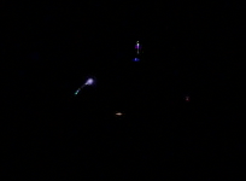
Figure 5: Portion of combined image from Nexus S in ¹³⁷Cs 100 mrem/hr field

Figure 6: Line finder processing of portion of combined image from Nexus S in ¹³⁷Cs 100 mrem/hr field

Two values are used for determining if something is an event or not and its type. These are the bright threshold and the bad_bright value. In order for the program to decided that some set of pixels are an event, at least one pixel needs to be over the bright threshold. In order for two bright pixels to be considered part of the same event, the line between them needs to have an average value that is higher than the bad_bright value.

The value of the bright and bad_bright can either be specified through command line arguments, or they can be automatically determined. The automatically determined bright value is $\bar{x}+5\sigma+16$ and the automatically determined $\bar{x}+3\sigma+16$ where $\bar{x}$ is the average pixel value and $\sigma$ is the standard deviation.

After determining the bright threshold, the program generates a list of bright points in the image. The points are chosen so that they are at least the exclude size of 2 pixels away from each other. The points are also adjusted within a few pixels to make sure that the brightest local pixel is chosen.

Next, the program calculates spanning trees between the bright pixels. For each iteration of the spanning tree algorithm, the program starts with a bright pixel that is currently unattached to a spanning tree. The remaining unattached bright pixels are iterated over, and the closest is attached to the spanning tree if it is closer than the maximum span length. If the closest to the currently attached set is greater than the maximum span length then the current spanning tree is done, and the next spanning tree will be worked on. The typical maximum span length is 10 pixels.

The program calculates statistics for each spanning tree, which are called groups. These statistics include the minimum and maximum x and y coordinates, the average brightness, the brightest pixel and the sum of the bright pixels. On a raw image, the sum of the bright pixels is related to the energy deposited, but on a color image these are only approximately related.

For each spanning tree, the program enumerates all the paths from one end to another end. For example, if the spanning tree ended up like a Y, there would be three ends and three paths. Each of these paths is a line. Statistics are printed for each line, such as total length and start and end locations.

For example, the line_finder program found five groups, three of which had lines in Figure 5. There were seven total lines in the image, and the debug output image is Figure 6, which shows the line segments in green, bright pixels that are part of a line in red, and bright pixels that are unattached in blue. The ratio of total lines to groups is correlated with the energy of the photon. The fraction of groups that have lines is also correlated to average incoming photon energy.

At the end, combined statistics are outputted such as total number of lines and total number of groups found and the number of groups that have lines.

9 Low Resolution Spectrum Results

Table 7: Most common gamma energies produced by tested nuclides (Voss, 2001)

Nuclide	Energies (keV)
241Am	60 (35.9%), 26 (2.4%), 33 (0.1%)
75Se	265 (59.8%), 136 (59.2%), 11 (47.5%) 280 (25.2%), 12 (7.3%), 1 (0.9 %)
192Ir	317 (82.85%), 468 (48.1%), 308 (29.68%), 296 (29.02%),67 (4.52%), 9 (4.1%), 65 (2.63%), 76 (1.97%)
137Cs	662 (89.98%), 32 (5.89%), 36 (1.39%), 5 (1%)
60Co	1173 (100%), 1332 (100

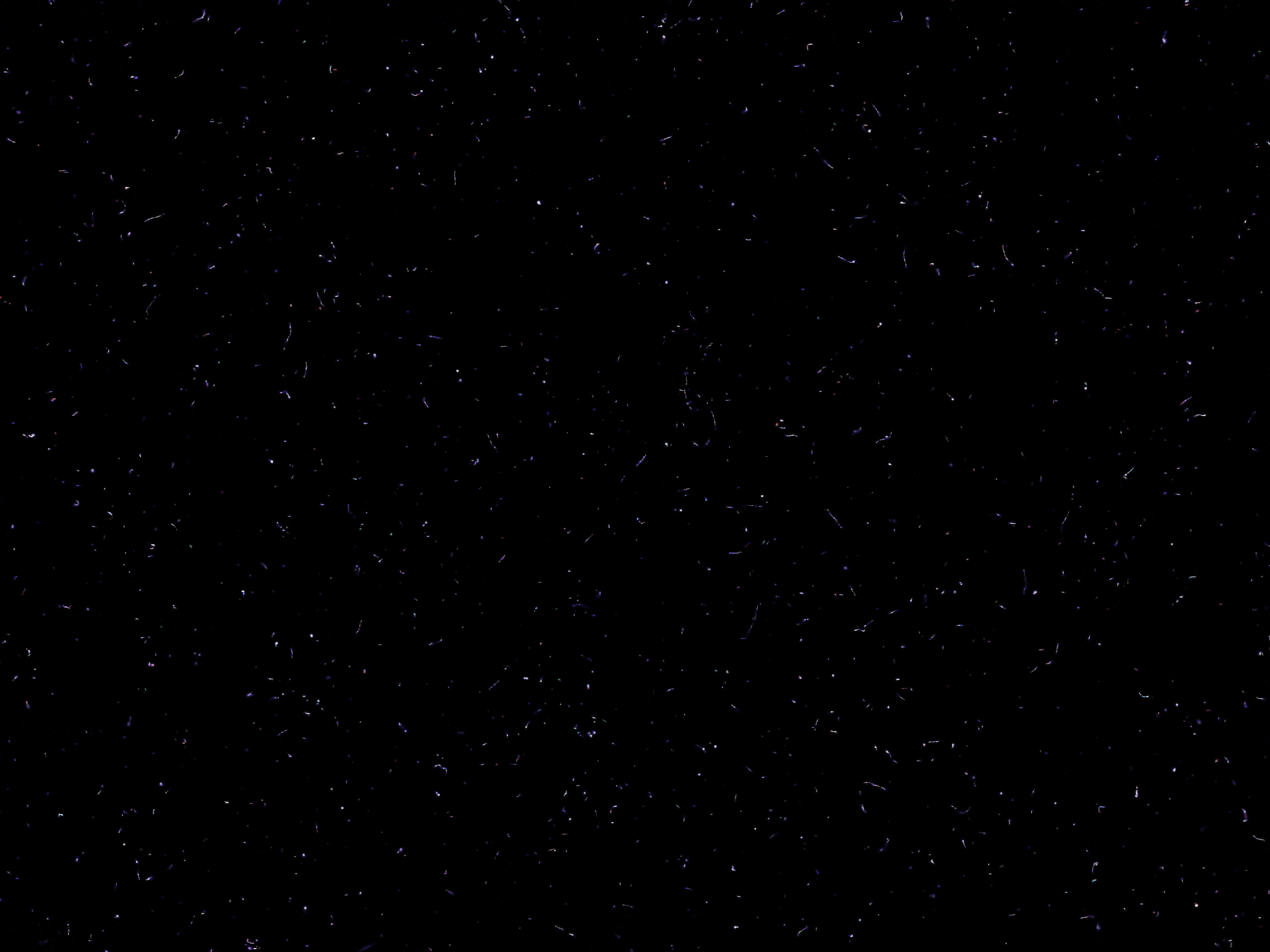
Figure 16: Example image from ¹³⁷Cs

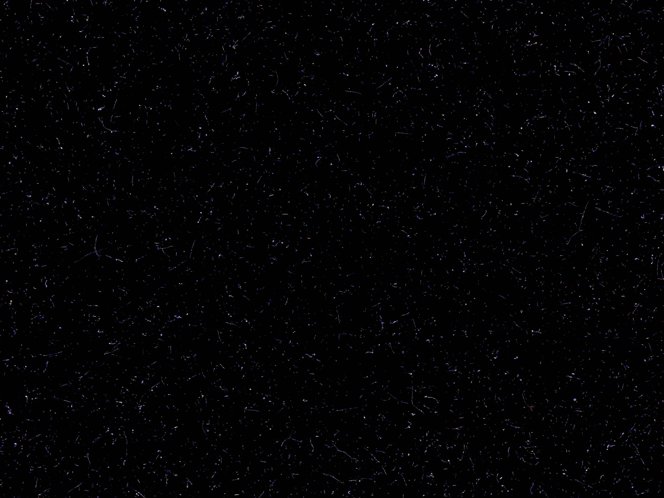
Figure 17: Example image from ⁶⁰Co

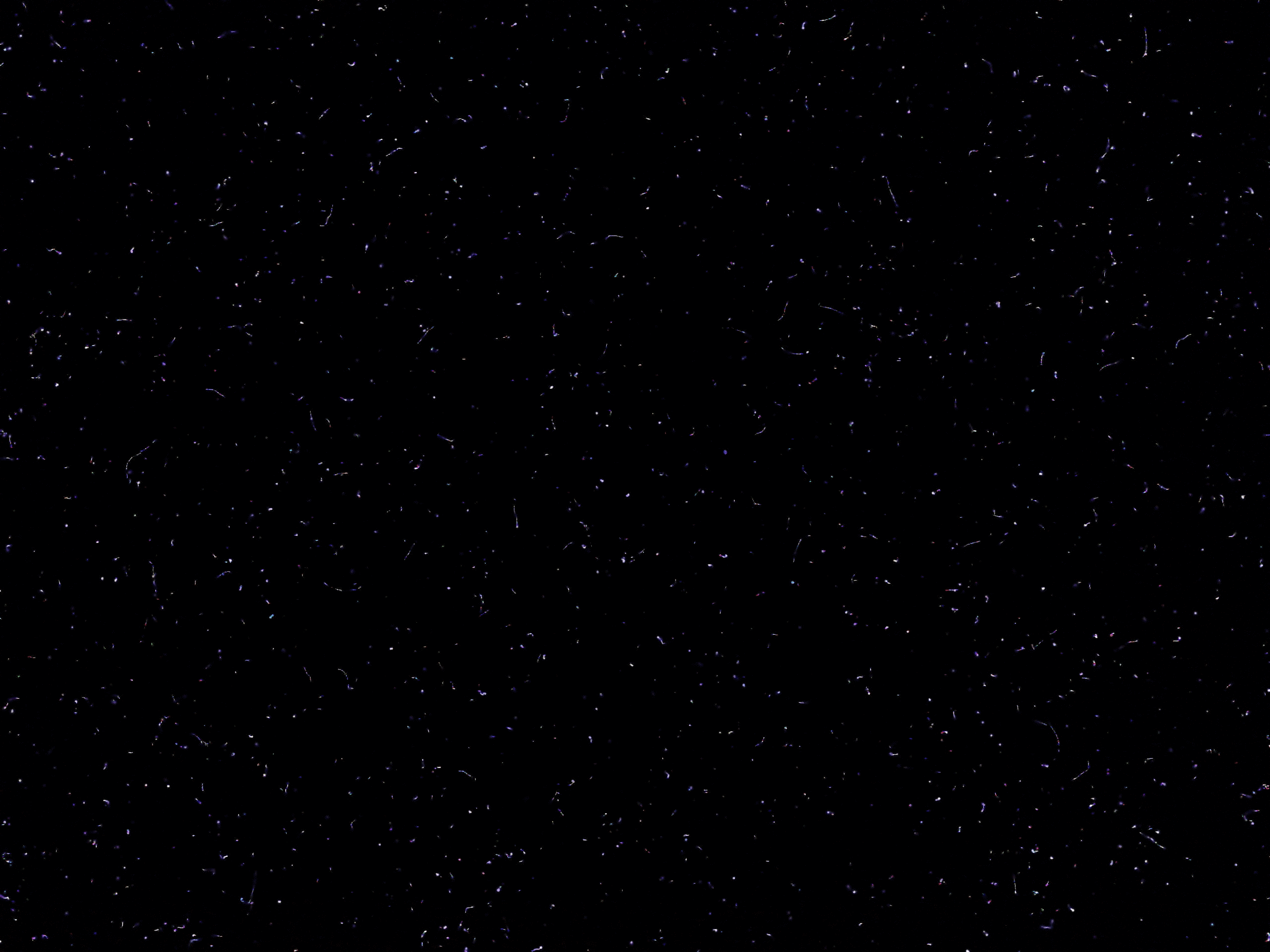
Figure 19: Example image from ¹⁹²Ir

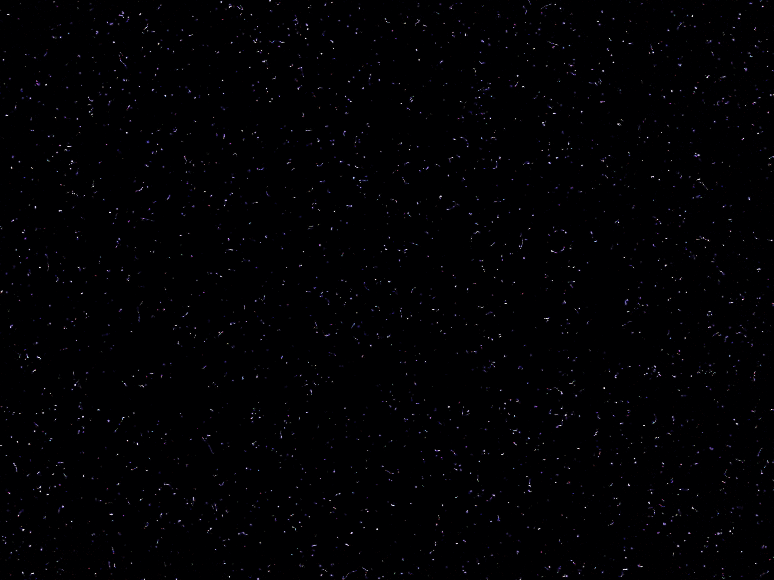
Figure 20: Example image from ⁷⁵Se

Several different curie level sources were tried at the INL site in August of 2012. The sources tried were a 1.3 Ci ²⁴¹Am source, a 1.3 Ci ¹³⁷Cs source (1.6 Ci at 7/8/2003), a 0.1 Ci ⁶⁰Co source (0.3 Ci at 7/8/2003), a 0.7 Ci ⁷⁵Se source (62.0 Ci at 6/21/2010) and a 1.3 Ci ¹⁹²Ir source (144.7 Ci at 2/23/2011). The common gamma energies are listed in Table 7. These were tried with the back camera facing the source, but with different distances ranging from 30 cm to 90 cm to the sources. For some of the experiments with the ²⁴¹Am source, the ¹³⁷Cs source and the ⁶⁰Co sources, steel plates up to 0.25 inches thick (0.635 cm) were put between the source and the cellphone to check the effect of shielding. For each single experiment count, 100 pictures were taken and then combined with the high-delta method, before being analyzed to determine groups and groups with lines fractions. Figures 16, 17, 18, 19, and 20 show example images from different sources.

The results from 138 experiments are in Figure 7 and the statistics from them in Table 8. From the data using the fraction of groups with lines, ⁶⁰Co and ¹³⁷Cs can be clearly distinguished from each other and from ⁷⁵Se and ²⁴¹Am. ¹⁹²Ir overlaps with ¹³⁷Cs, and ⁷⁵Se and ²⁴¹Am overlap. The fraction of groups with lines decreases as the average energy of the gamma rays increases. Figure 8 shows the relationship between the average energy of the nuclide and the fraction of groups with lines.

Table 8: Fraction of Groups with Lines Statistics

	75Se	192Ir	137Cs	60Co	241Am
Mean	0.659	0.578	0.527	0.415	0.717
Standard Deviation	0.009	0.013	0.028	0.021	0.043
Minimum	0.642	0.557	0.474	0.370	0.625
Maximum	0.668	0.594	0.564	0.447	0.833
Count	6	6	39	51	36

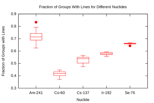
Figure 7: Nexus S, 1 foot to 3 feet away from various curie level sources

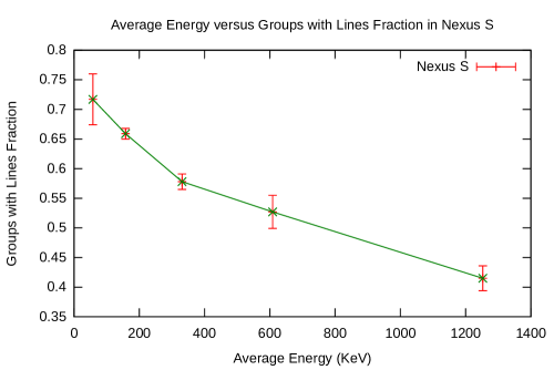
Figure 8: Comparison of average nuclide energy with fraction of groups with lines and standard deviation error bars

10 Rotation Results

Changing the angle of the incoming gamma rays changes what materials the gamma rays travel through to get to the sensor. For example, at certain angles the gamma rays will travel through the battery before reaching the camera. This material can attenuate the gamma rays. The interaction also can generate high energy electrons that are detected by the CMOS sensor. From Equation 1 the electrons scattered from Compton scattering have an angular energy dependence. These two effects changes both the number of events that are seen and the types of features that are seen. A Nexus S phone was placed in a 10 R/hr field generated from ¹³⁷Cs and a separate 10 R/hr field generated from ⁶⁰Co at the INL’s HPIL. The phone was placed vertically, either taped to a cardboard box with the top of the phone and the camera above the box as in Figure 13 or with the back camera against a 30.5 x 30.5 x 15.2 cm (12 x 12 x 6 inch) block of Lucite (Polymethyl methacrylate) as in Figure 14.

Table 9: Nexus S Rotation Data Back Camera

		Back Camera Lucite				Back Camera Plain
Nuclide	Degrees	Groups	GwL	GwLL	MLL	Groups	GwL	GwLL	MLL
137Cs	0	33699	15422	3415	69.69	78143	32324	7676	79.40
137Cs	90	57803	28188	7041	99.27	52068	25246	6335	86.24
137Cs	180	78089	33335	7789	75.51	72336	29394	7070	99.62
137Cs	270	58905	28665	7044	97.13	58223	28111	7081	80.72
60Co	0	52591	18649	4004	70.88	99868	32826	7383	115.07
60Co	90	75730	30407	7298	83.80	73267	29285	7064	128.98
60Co	180	91483	31471	7155	89.08	88264	29075	6494	102.07
60Co	270	79504	31720	7598	100.65	75897	29807	7117	106.89

Table 10: Nexus S Rotation Data Front Camera

		Front Camera Lucite				Front Camera Plain
Nuclide	Degrees	Groups	GwL	GwLL	MLL	Groups	GwL	GwLL	MLL
137Cs	0	254	92	6	21.67	515	165	7	22.61
137Cs	90	445	150	16	20.54	433	126	9	19.30
137Cs	180	609	184	17	17.06	534	165	18	18.06
137Cs	270	435	127	12	17.46	356	111	8	25.21
60Co	0	245	78	3	15.39	458	118	13	25.32
60Co	90	437	117	8	19.34	395	95	4	15.86
60Co	180	497	130	10	21.11	454	109	8	16.39
60Co	270	447	133	10	14.57	368	98	6	14.53

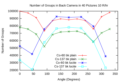
Figure 9: Nexus S Angular Groups 10 R/hr, 40 pictures back camera 1.0 sec exposure

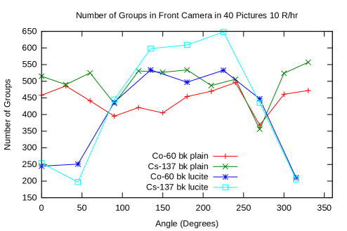
Figure 10: Nexus S Angular Groups 10 R/hr, 40 pictures front camera 0.125 sec exposure

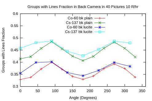
Figure 11: Nexus S Angular Fraction of Groups with Lines, 10 R/hr, 40 pictures back camera 1.0 sec exposure

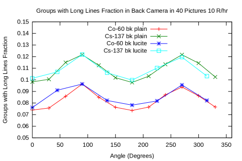
Figure 12: Nexus S Angular Fraction of Groups with Long Lines, 10 R/hr, 40 pictures back camera 1.0 sec exposure

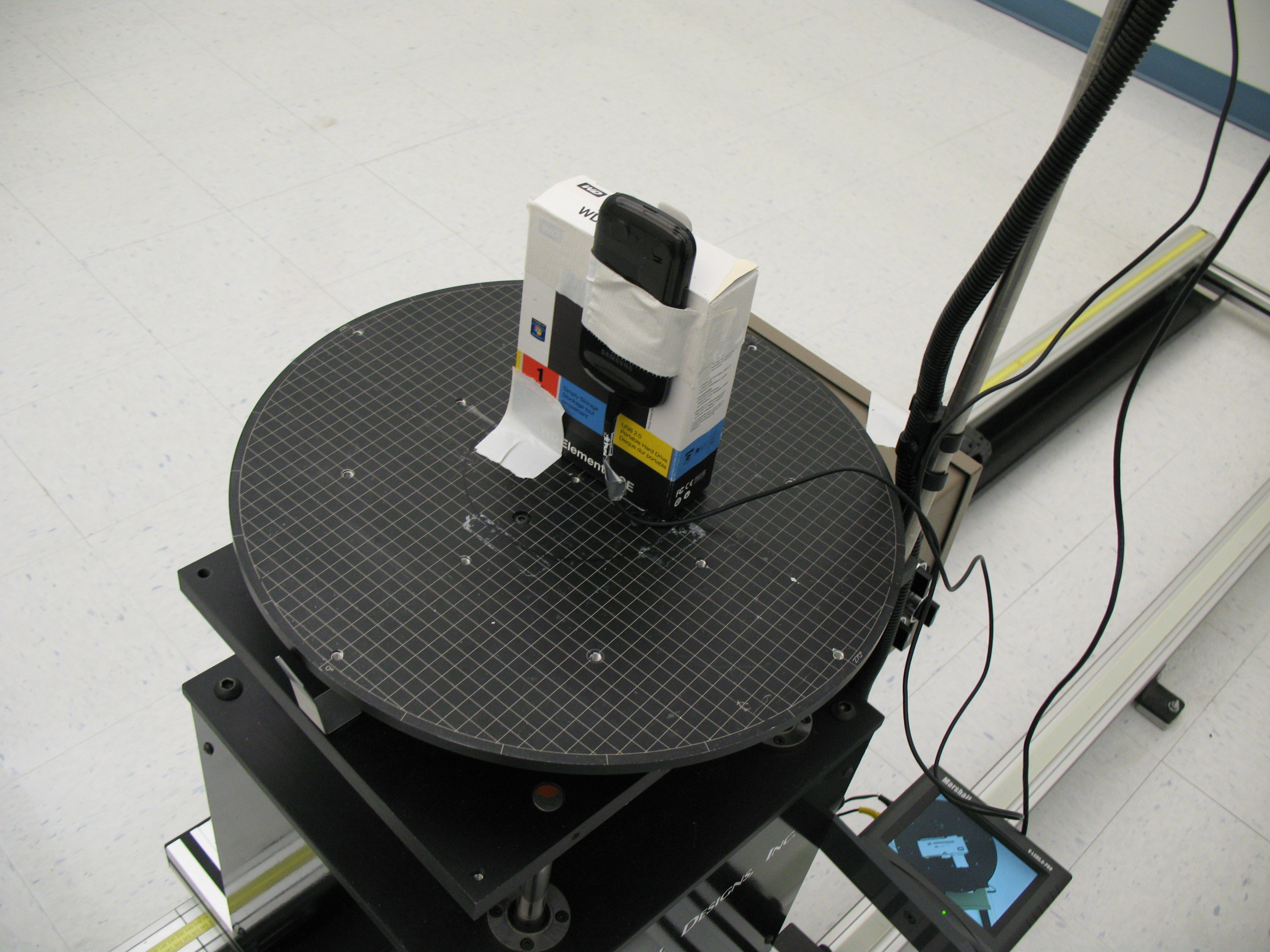
Figure 13: Nexus S Plain 0 degrees

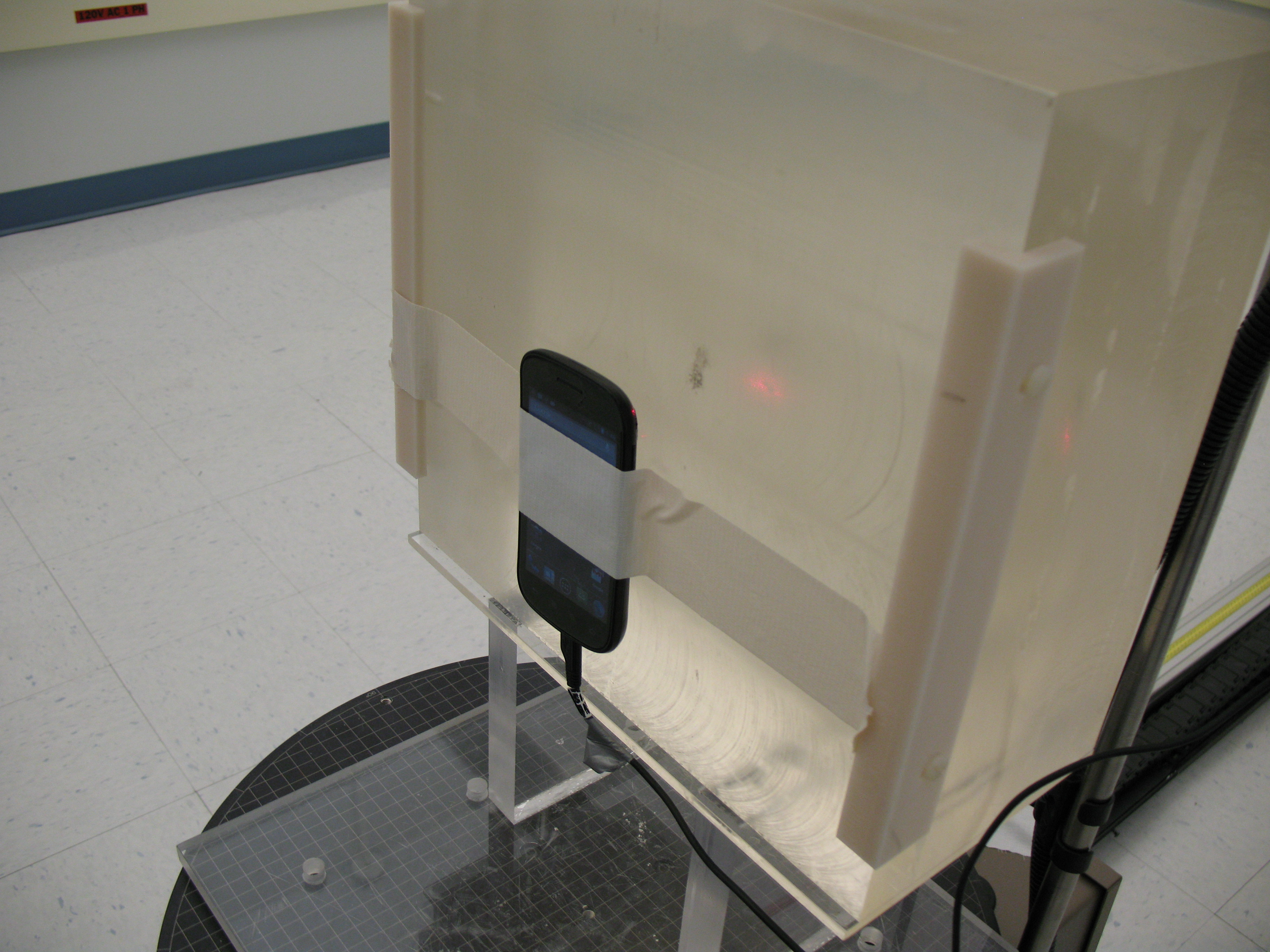
Figure 14: Nexus S Against Lucite 180 degrees

For each of the results in this section and the next, 40 pictures were taken with both the front and the back camera. Then, a background picture was generated using the highest value found that was less than the pixel component’s $\bar{x}+2\sigma$ as in Equation 2. The background picture was then subtracted from each of the 40 pictures, and then line finding and group counting were done on the images.

Tables 9 and 10 provide the summary data for the four different directions (where 0 degrees is the back camera facing the source). The data provided is the total number of groups (See also Figures 9 and 10), the number of groups with lines greater than 2 pixels long (GwL) (See also Figure 11), the number of groups with lines greater than 10 pixels long (GwLL) (See also Figure 12), and the maximum line length found in all the groups (MLL). From the groups data in the tables and in Figures 9 and 10, it can be seen that the Lucite block attenuates the source strength resulting in lower numbers of groups compared to plain air near 0 degrees, but increases the group count from scattering when the cell phone camera is between or beside the lucite. The lucite testing was done to determine the effect of carrying the cellphone next to a human since the lucite is made of hydrogen, carbon and oxygen. Depending on whether the human is between the phone and the source, or the phone is between the human and the source, the measured dose rate will either be decreased or increased. For the in plain air data, the dose differences when rotated are caused by different attenuation and scattering from the internal cellphone components.

Examining the fraction of groups with lines (Figure 11) and the fraction of groups with long lines (Figure 12) leads to important conclusions. A key detail to note is the fractions vary with the incoming gamma angle. At any individual angle, the fractions of groups with lines are different, so when the incoming angle is known, the nuclides ⁶⁰Co and ¹³⁷Cs can be distinguished. However, because the data nearly overlap between the ⁶⁰Co and the ¹³⁷Cs at different incoming angles, if the incoming gamma angle is not known and cannot be determined, the nuclides cannot be distinguished. However, the cellphone does have both multiple cameras and orientation sensors; it is at least conceivable that this difference in fraction might be able to be used to determine the direction to the gamma source. This would require accurate position registration with the time when the picture was taken, and significant amounts of data transferred to the server, so it may not be practical. The ratio between dose detected at the front and back camera might be usable for direction finding as well, but the lower resolution on the front camera would require more data to be used.

11 Dose Results

Using the same test protocol as the previous section, the response to different dose rates was tested. In this case different phones were placed into gamma fields ranging from 1 mrem/hr to 100,000 mrem/hr. As can be seen from Table 14, the Nexus S has the highest groups per mrem/hr per image, which indicates that it is the best for detecting radiation on a per image basis. From Figure 15 there is clear correspondence between the number of groups and the dose rate. The figure also shows that the Galaxy SIII has excessive noise in the camera that is not compensated for by the existing noise processing in CellRad. Table 11 provides data gathered from two different Nexus S phones, which indicates that phone to phone intra-model variance is fairly low, compared to between-model variance.

Table 11: Comparison of two Nexus S phones’ group count from data in 10,000 mrem/hr field and one background case

Case	3334…	3231…	% Change
background	0	0	NA
60Co 0∘	99868	102965	3.0%
60Co 90∘	73267	75457	2.9%
60Co 180∘	88264	90614	2.6%
137Cs 0∘	78143	78341	0.3%
137Cs 90∘	52068	55235	5.7%
137Cs 180∘	72336	73850	2.1%

Table 12: Phones Dose Tested Settings

Name	Back Camera	Time (s)	Settings
Samsung Nexus S	2560x1920	1.0	-m fireworks -e 0
Samsung Galaxy Nexus	2592x1944	0.125	-m night -e 0
Samsung Galaxy SIII	3264x2448	0.125	-m night -e 0
LG Nexus 4	3264x2448	1.0	-m steadyphoto -e 12

Table 13: Phones Dose Tested Bright and Bad_bright Settings

Name	Bright	Bad_bright
Samsung Nexus S	64	48
Samsung Galaxy Nexus	100	80
Samsung Galaxy SIII	48	32
LG Nexus 4	48	32

Table 14: Groups Per mrem Per image

Phone	average	min	max	1 R/hr 60Co	1 R/hr 137Cs
Nexus S	0.20295	0.12708	0.2753	0.2753	0.2106
Galaxy SIII	0.13618	0.01185	1.1	0.013	0.0133
Nexus 4	0.01198	0.009	0.025	0.009	0.012125
Nexus Galaxy	0.00450	0	0.0075	0.009	0.004875

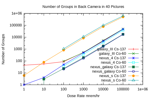
Figure 15: Dose to Number of Groups

12 Conclusion

This project has demonstrated that a smartphone with a camera can be used as a low sensitivity dose rate meter. If the radiation is coming from a known direction, with sufficient data, limited spectrum information can be determined. There are better detectors than a cellphone camera will likely every be, but there are many more cellphones around than high-quality radiation detectors, which means there are times when the cellphone can be the best detector available.

13 Acknowledgments

This manuscript has been authored by Battelle Energy Alliance, LLC under Contract No. DE-AC07-05ID14517 with the U.S. Department of Energy. The United States Government retains and the publisher, by accepting the article for publication, acknowledges that the United States Government retains a nonexclusive, paid-up, irrevocable, worldwide license to publish or reproduce the published form of this manuscript, or allow others to do so, for United States Government purposes.

Work supported by the U.S. Department of Energy, Nuclear Nonproliferation and Security Administration, and the U.S. Department of Defense, Office of Secretary Of Defense under DOE Idaho Operations Office Contract DE-AC07-05ID14517.

Many thanks to: Project Leaders Steven H. McCown and Gus Caffrey, Technical discussions from Shane Hansen, Woo Y. Yoon, Daren R. Norman, Hope Forsmann, Glenn Knoll, Edward H. Seabury, Thayne C. Butikofer, Paul K. Halversen, John Richardson, Scott B. Brown and Ryan C. Hruska. Experimental support and technical discussion from Christopher P. Oertel, Glenna L. Seal, Norman A. Rhodehouse, Laurel Hill, Byron Christiansen, Bryce J. Woodbury, Gary Engelstad, Jennifer A. Turnage, John R. Giles, and Kent L. Brinker. In addition to other contributions, Dr. Carl A. Kutsche suggested that the difference in fraction of groups with lines with incoming angle could potentially be used to determine direction to the gamma source.

Figure 18: Example image from ²⁴¹Am

References

- Cogliati (2010) Joshua Cogliati. Determining camera gain in room temperature cameras. 2010. URL http://www.inl.gov/technicalpublications/Documents/4702567.pdf. INL/EXT-10-20072.
- Derr et al. (2012) Kurt Derr, Misty Benjamin, and Carl Kutsche. Cellphone-based radiation warning system - idaho national laboratory research fact sheet. 2012. URL http://www.inl.gov/research/cellphone-based-radiation-warning-system/. 12-GA50627.
- Drukier et al. (2011) Gordon A. Drukier, Eric P. Rubenstein, Peter R. Solomon, Marek A. Wójtowicz, and Michael A. Serio. Low cost, pervasive detection of radiation threats. 2011 IEEE International Conference on Technologies for Homeland Security, November 2011. doi: 10.1109/THS.2011.6107897.
- Gabel (2012) Marty Gabel. Can the gammapix android app really save your life? 2012. URL http://m.androidapps.com/tech/articles/11838-can-the-gammapix-android-app-really-save-your-life.
- Holland (1996) A.D. Holland. X-ray spectroscopy using mos ccds. Nuclear Instruments and Methods in Physics Research A, 337:334–339, 1996.
- Holst (1998) Gerald C. Holst. CCD Arrays, Cameras, and Displays. SPIE Press, 1998. ISBN 0-9640000-4-0.
- Ishiwatari et al. (2006) T. Ishiwatari, G. Beer, A.M. Bragadireanu, M. Cargnelli, C. Curceanu (Petrascu), J.-P. Egger, H. Fuhrmann, C. Guaraldo, M. Iliescu, K. Itahashi, M. Iwasaki, P. Kienle, B. Lauss, V. Lucherini, L. Ludhova, J. Marton, F. Mulhauser, T. Ponta, L.A. Schaller, D.L. Sirghi, F. Sirghi, P. Strasser, and J. Zmeskal. New analysis method for ccd x-ray data. Nuclear Instruments and Methods in Physics Research A, 556:509–515, 2006. doi: 10.1016/j.nima.2005.10.105.
- Janesick (2001) James R. Janesick. Scientific Charge-Coupled Devices. SPIE Press, 2001. ISBN 0-8194-3698-4.
- Kim et al. (2006) Young Soo Kim, Gyuseong Cho, and Jun-Hyung Bae. Analysis of noise characteristics for the active pixels in cmos image sensors for x-ray imaging. Nuclear Instruments & Methods in Physics Research A, 565:263–267, 2006. doi: 10.1016/j.nima.2006.05.008.
- Knoll (2000) Glenn F. Knoll. Radiation Detection and Measurement, Third Edition. John Wiley & Sons, Inc., 2000. ISBN 0-471-07338-5.
- MacDonald et al. (1997) J.H. MacDonald, K. Wells, A.J. Reader, and R.J. Ott. A ccd-based tissue imaging system. Nuclear Instruments and Methods in Physics Research A, 392:220–226, 1997.
- Mayo (1998) Robert M. Mayo. Introduction to Nuclear Concepts for Engineers. American Nuclear Society, 1998. ISBN 0-89448-454-0.
- mike449 (2008) mike449. Cell phone radiation detectors proposed to protect against nukes: Using the built-in camera? 2008. URL http://mobile.slashdot.org/comments.pl?sid=429956.
- Quick (2011) Darren Quick. Wikisensor app turns an iphone into a peripheral-free radiation detector. 2011. URL http://www.gizmag.com/wikisense-radiation-detector-app/20294/.
- Voss (2001) James Tom Voss. Los Alamos Radiation Monitoring Notebook. Los Alamos National Laboratory, 2001. LA-UR-00-2584.
- Yadid-Pecht and Etienne-Cummings (2004) Orly Yadid-Pecht and Ralph Etienne-Cummings, editors. CMOS Imagers: From Phototransduction to Image Processing. Kluwer Academic Publishers, 2004. ISBN 1-4020-7961-3.