Context-Aware Hypergraph Construction for Robust Spectral Clustering

Abstract

Spectral clustering is a powerful tool for unsupervised data analysis. In this paper, we propose a context-aware hypergraph similarity measure (CAHSM), which leads to robust spectral clustering in the case of noisy data. We construct three types of hypergraph—the pairwise hypergraph, the $k$-nearest-neighbor ($k$NN) hypergraph, and the high-order over-clustering hypergraph. The pairwise hypergraph captures the pairwise similarity of data points; the $k$NN hypergraph captures the neighborhood of each point; and the clustering hypergraph encodes high-order contexts within the dataset. By combining the affinity information from these three hypergraphs, the CAHSM algorithm is able to explore the intrinsic topological information of the dataset. Therefore, data clustering using CAHSM tends to be more robust. Considering the intra-cluster compactness and the inter-cluster separability of vertices, we further design a discriminative hypergraph partitioning criterion (DHPC). Using both CAHSM and DHPC, a robust spectral clustering algorithm is developed. Theoretical analysis and experimental evaluation demonstrate the effectiveness and robustness of the proposed algorithm.

1 Introduction

Spectral clustering is an effective means of clustering data with complex topological structure [10, 11, 15, 8, 12, 16, 13, 9, 31, 34, 35, 36]. It plays an important role in unsupervised learning from data, and therefore has a wide range of applications, including circuit layout [1, 2], load balancing [3], image segmentation [4, 5, 6, 7, 14], motion segmentation [25], video retrieval [26], etc. Typically, the affinity relationships between data samples are modeled by a graph, and therefore spectral clustering aims to optimize a graph partitioning criterion for data clustering based on local vertex similarities. However, there are still several unsolved issues for traditional spectral clustering methods: i) how to automatically discover the number of clusters; ii) how to correctly choose the scaling parameter for graph construction; iii) how to counteract the adverse effect of noise or outliers; and iv) how to incorporate different types of information to enhance the clustering performance.

In the literature, Zelnik-Manor and Perona [11] attempt to address issues i) and ii) by designing a local scaling mechanism, which adaptively calculates the affinity matrix and explores the intrinsic structural information on the energy eigenvalue spectrum of the normalized graph Laplacian to discover the number of clusters. However, this local scaling mechanism is susceptible to noise or outliers. Following [11], Li et al. [15] propose a noise robust spectral clustering (NRSC) algorithm to resolve issues i) and iii). The proposed NRSC algorithm can automatically estimate the number of clusters via computing the largest eigenvalue gap of the normalized graph Laplacian. In addition, the proposed NRSC algorithm maps the original data samples (vertices) into a new space, in which the clusters have a higher intra-cluster compactness and inter-cluster separability. If the noisy data samples are weakly interconnected with each other, this mapping relocates the noisy data samples around the origin of the new space. This usually results in a compact noise cluster. However, the real-world data samples (e.g., images and videos) within a cluster are often not densely interconnected due to problems with the visual feature description. Therefore, the mapping may lead to topological information loss for the clusters. As a result, the weakly interconnected samples in the ordinary clusters are also relocated around the origin of the new space. This may result in low separability between clusters.

More recently, hypergraph analysis [17, 18] has emerged as a popular tool for addressing issues iii) and iv). The fundamental idea of hypergraph analysis is to explore the underlying affinity relationships among vertices by constructing a hypergraph with a variety of hyperedges that capture affinity. This has been applied to many domains such as image matching [19], multi-label classification [20], video object segmentation [21], and image retrieval [22]. For example, Sun et al. [20] carry out hypergraph construction by sequentially introducing new vertices into existing hyperedges using clique expansion or star expansion. Huang et al. [22] propose a probabilistic hypergraph model that softly assigns a vertex to a hyperedge according to the similarity between the vertex and the centroid of the hyperedge.

Motivation and contribution In general, most existing spectral clustering algorithms only focus on the pairwise interactions between vertices. In other words, the pairwise similarity between two vertices is only based on the individual vertices themselves. If a vertex is corrupted, this pairwise similarity can change significantly. Consequently, their true affinity may not be stably represented. Thus, designing a robust similarity measure is one of the key problems in data clustering.

Here, we show that the high-order contextual information on vertices can help alleviate this problem. Contexts are groups of vertices that share some common properties. Once contexts have been computed, the vertex similarity measure depends on not only two individual vertices but also their corresponding contexts. The similarity measure that includes contextual information is much more stable because it takes into account local grouping and neighborhood information of each vertex. When a single vertex is corrupted, the high-order contextual similarity can still provide complementary information to counteract the impact of the corruption.

Motivated by this observation, we propose a robust spectral clustering algorithm based on a context-aware hypergraph similarity measure. We use three different types of hypergraphs: pairwise hypergraph, $k$-nearest-neighbor ($k$NN) hypergraph, and high-order over-clustering hypergraph. The pairwise hypergraph is capable of encoding pairwise affinity information on vertices. In contrast, the $k$NN hypergraph and the over-clustering hypergraph capture the underlying manifold structure on vertices by modeling their high-order neighborhood and contextual grouping properties, respectively. By combining these hypergraphs, we obtain the context-aware hypergraph similarity measure that characterizes the intrinsic connectivity relationships among vertices, resulting in the clustering robustness in the case of noise or outlier corruption.

The main contributions of this work are therefore three-fold.

• We introduce a high-order context into the spectral clustering process. The high-order context of a vertex is defined as a set of vertices with similar properties to the vertex. Each vertex in a context is influenced by other vertices in the same context.

• The problem of building the high-order context is converted to that of hypergraph construction, which encodes the local affinity information using different types of hypergraphs. To this end, we design three types of hypergraphs to encode the pairwise, neighboring, and local grouping information on vertices. Based on these hypergraphs, we further propose a context-aware hypergraph similarity measure (CAHSM) to capture the intrinsic topological information on vertices. In essence, CAHSM is a generalization of traditional similarity measures, and aims to utilize the hypergraph context to explore the underlying affinity relationships between vertices.

• We propose a discriminative hypergraph partitioning criterion (DHPC) to characterize the intra-cluster compactness and the inter-cluster separability of vertices. By maximizing the DHPC, we effectively capture the discriminative information on vertices. The optimization of DHPC can be relaxed into a trace-ratio maximization problem. Using both CAHSM and DHPC, we develop a pairwise+$k$NN+over-clustering hypergraph spectral clustering algorithm (referred to as PKO+HSC) for data clustering.

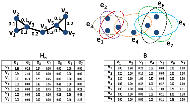
Figure 1: Illustration of the $k$NN hypergraph construction. The top-left subfigure shows the pairwise edge between any vertex and its two nearest neighbors; the top-right subfigure displays the associated hypergraph structure whose hyperedges (highlighted by ellipses of different colors) consist of each vertex and its two nearest neighbors; the bottom-left subfigure shows the $k$NN hypergraph incidence matrix $H_{n}$; and the bottom-right subfigure exhibits the $k$NN hypergraph similarity matrix $B$.

2 Context-aware hypergraph construction

In what follows, we first discuss how to construct a robust hypergraph similarity measure using three different types of hypergraphs, and then describe a discriminative hypergraph partitioning criterion for data clustering.

2.1 Context-aware hypergraph similarity measure

In order to effectively explore the high-order affinity relationships among vertices, we propose a hypergraph construction mechanism based on three types of hypergraphs, which are the pairwise hypergraph, the $k$-nearest-neighbor ($k$NN) hypergraph, and the over-clustering hypergraph. The pairwise hypergraph reflects the pairwise relationships between vertices; the $k$NN hypergraph characterizes the neighboring information on vertices, and the over-clustering hypergraph captures the local grouping relationships among vertices. By combining these three types of hypergraphs, the proposed hypergraph construction mechanism is capable of exploring the underlying high-order affinity relationships among vertices.

1) Pairwise hypergraph. For easy exposition, let $\mathbb{Z}=\{\mathbf{z}_{i}\}_{i=1}^{N}$ denote a sample set. Based on $\mathbb{Z}=\{\mathbf{z}_{i}\}_{i=1}^{N}$, we create a pairwise graph $G_{p}$ with $N$ vertices. Mathematically, the graph $G_{p}$ can be denoted as $G_{p}=(\mathbb{V},E_{p},W_{p})$, where $\mathbb{V}=\{v_{i}\}_{i=1}^{N}$ is the vertex set corresponding to $\{\mathbf{z}_{i}\}_{i=1}^{N}$, $E_{p}\subseteq\mathbb{V}\times\mathbb{V}$ is the edge set containing all possible pairwise edges, and $W_{p}$ is the edge-weight function returning the affinity value between two vertices. In practice, the graph $G_{p}$ is formulated as a weighted similarity matrix $A=(a_{ij})_{N\times N}$:

$$a_{ij}=\left\{\begin{array}[]{cc}W_{p}(v_{i},v_{j})&\mbox{if}\thickspace(v_{i},v_{j})\in E_{p},\\ 0&\mbox{otherwise},\end{array}\right.{}$$ (1)

where $W_{p}(v_{i},v_{j})=\mathcal{G}(\mathbf{z}_{i},\mathbf{z}_{j})$ is a kernel function used for measuring the similarity between $\mathbf{z}_{i}$ and $\mathbf{z}_{j}$. Note that the above procedure of graph creation is independent of the choice of kernel functions. In other words, it is easy to incorporate various kernel functions into the above graph creation process.

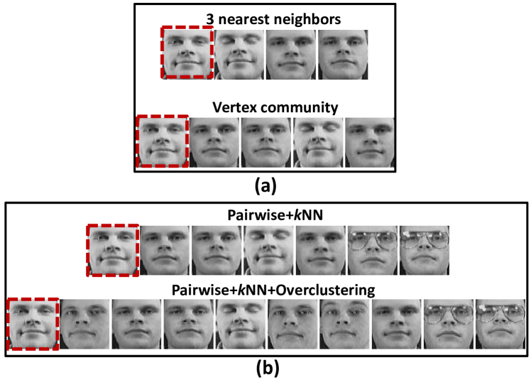
Figure 2: Illustration of different hypergraph concepts and hypergraph clustering results based on different hypergraph similarity measures. Specifically, the upper part of (a) shows the 3 nearest neighbors of the face image highlighted by the dot-dashed bounding box; the lower part of (a) displays a vertex community that is a high-order context of the face image highlighted by the dot-dashed bounding box; the upper and lower parts of (b) respectively exhibit the clustering results containing the face image (highlighted by the dot-dashed bounding box) using pairwise+$k$NN and pairwise+$k$NN+over-clustering hypergraph similarities (respectively corresponding to PK+HSC and the proposed PKO+HSC). Clearly, the proposed pairwise+$k$NN+over-clustering similarity measures performs best.

According to the hypergraph theory, the pairwise graph $G_{p}$ is merely a special hypergraph whose hyperedge cardinality equals 2. Therefore, we reformulate $G_{p}$ using the hypergraph terminologies. As a generalization of a traditional pairwise graph, a hypergraph is composed of many hyperedges, and each hyperedge corresponds to a set of vertices which have some common properties. Mathematically, these hyperedges are generally associated with a hypergraph incidence matrix $H_{p}=(h_{p}(v_{i},e^{p}_{\ell}))_{|\mathbb{V}|\times|E_{p}|}$:

$$h_{p}(v_{i},e^{p}_{\ell})=\left\{\begin{array}[]{ll}1,&\mbox{if}\thickspace v_{i}\in e^{p}_{\ell},\\ 0,&\mbox{otherwise},\end{array}\right.{}$$ (2)

where $e^{p}_{\ell}=(v_{m},v_{n})$ is the $\ell$-th hyperedge of $E_{p}$. In order to measure the degree of the within-hyperedge vertices belonging to the same cluster, we introduce the notion of the pairwise hyperedge weight, which is defined as the pairwise similarity of the vertices in each hyperedge. So we can define the pairwise hypergraph similarity as:

$$u_{ij}=\underset{e^{p}_{\ell}\in E_{p}}{\sum}\eta_{p}(e^{p}_{\ell})h_{p}(v_{i},e^{p}_{\ell})h_{p}(v_{j},e^{p}_{\ell})=a_{ij},{}$$ (3)

where $\eta_{p}(e^{p}_{\ell})$ is the corresponding hyperedge weight of $e^{p}_{\ell}=(v_{m},v_{n})$ such that $\eta_{p}(e^{p}_{\ell})=a_{mn}$. As a result, we have a weighted hypergraph similarity matrix $U=(u_{ij})_{N\times N}$ that characterizes the pairwise affinity relationships between vertices. For simplicity, the resulting pairwise hypergraph similarity matrix is represented as its corresponding matrix form:

$$U=H_{p}\Sigma_{p}H_{p}^{T}=A,{}$$ (4)

where $\Sigma_{p}$ is a diagonal matrix whose diagonal elements are denoted as $(\eta_{p}(e^{p}_{\ell}))_{e^{p}_{\ell}\in E_{p}}$.

2) $k$-nearest-neighbor ($k$NN) hypergraph. Based on the neighboring information on vertices, we further define a $k$NN hypergraph $G_{n}$, as shown in Fig. 1. For each vertex $v_{\ell}$, we search its corresponding $k$ nearest neighbors $\{v_{q}|v_{q}\in\mathcal{N}_{v_{\ell}}^{k}\}$ (as shown in Fig. 2(a)), and then use these nearest neighbors to form a $k$NN hyperedge $e_{\ell}^{n}$. By concatenating all the $k$NN hyperedges, a $k$NN hyperedge set is generated as $E_{n}=\{e_{\ell}^{n}\}_{\ell=1}^{N}$, as illustrated in Fig. 3. To characterize the vertex-to-hyperedge membership, we define an indicator function as:

$$\mathbb{I}(v_{i},e^{n}_{\ell})=\left\{\begin{array}[]{cc}1,&\mbox{if}\thickspace v_{i}\in e^{n}_{\ell},\\ 0,&\mbox{otherwise},\end{array}\right.{}$$ (5)

Based on this indicator function, we design a hypergraph model for softly assigning a vertex to each hyperedge:

$$h_{n}(v_{i},e^{n}_{\ell})=\frac{a_{\ell i}\sqrt{\mathbb{I}(v_{i},e^{n}_{\ell})}}{\sqrt{\sum_{t=1}^{N}\delta_{t}\mathbb{I}(v_{i},e^{n}_{t})a_{ti}^{2}}},{}$$ (6)

where $\delta_{t}$ is the hyperedge weight associated with the $t$-th hyperedge $e^{n}_{t}$ such that $\delta_{t}=\frac{1}{|e^{n}_{t}|}\sum_{j\in\{r|v_{r}\in e^{n}_{t}\}}a_{tj}$, and $a_{\ell i}$ represents the vertex-to-hyperedge similarity between $v_{i}$ and the $\ell$-th $k$NN hyperedge $e_{\ell}^{n}$. Specifically, $e_{\ell}^{n}$ is composed of a centroid vertex $v_{\ell}$ and its corresponding $k$ nearest vertices. Based on Eq. (1), the vertex-to-hyperedge similarity $a_{\ell i}$ is computed as the pairwise similarity between $v_{i}$ and $v_{\ell}$. As a result, we obtain a $k$NN hypergraph incidence matrix $H_{n}=(h_{n}(v_{i},e^{n}_{\ell}))_{|\mathbb{V}|\times|E_{n}|}$ for capturing the vertex-to-hyperedge relationships. Based on $H_{n}$, a $k$NN hypergraph similarity $b_{ij}$ between $v_{i}$ and $v_{j}$ is derived as:

$$\begin{array}[]{ll}b_{ij}&=\underset{e^{n}_{\ell}\in E_{n}}{\sum}\delta_{\ell}\hskip 1.42271pth_{n}(v_{i},e^{n}_{\ell})h_{n}(v_{j},e^{n}_{\ell})\\ &=\frac{\sum_{\ell=1}^{N}(a_{\ell i}\sqrt{\mathbb{I}(v_{i},e^{n}_{\ell})\delta_{\ell}})(a_{\ell j}\sqrt{\mathbb{I}(v_{j},e^{n}_{\ell})\delta_{\ell}})}{\sqrt{\sum_{t=1}^{N}a_{ti}^{2}(\sqrt{\mathbb{I}(v_{i},e^{n}_{t})\delta_{t}})^{2}}\sqrt{\sum_{t=1}^{N}a_{tj}^{2}(\sqrt{\mathbb{I}(v_{j},e^{n}_{t})\delta_{t}})^{2}}}\\ &=\frac{\left<\mathbf{x}_{i},\mathbf{x}_{j}\right>}{\|\mathbf{x}_{i}\|\|\mathbf{x}_{j}\|},\end{array}{}$$ (7)

where $\mathbf{x}_{m}=\left(a_{\ell m}\sqrt{\mathbb{I}(v_{m},e^{n}_{\ell})\delta_{\ell}}\right)_{\ell=1}^{N}$, $<\cdot,\cdot>$ is the inner product operator, and $\|\cdot\|$ is the 2-norm. Indeed, $\mathbf{x}_{m}$ is a vertex-to-hyperedge feature vector that characterizes the correlation between $v_{m}$ and the $k$NN hyperedges. For example, the $\ell$-th element of $\mathbf{x}_{m}$ contains two terms: $a_{\ell m}$ and $\sqrt{\mathbb{I}(v_{m},e^{n}_{\ell})\delta_{\ell}}$. The first term $a_{\ell m}$ is the pairwise similarity between $v_{m}$ and the vertex $v_{\ell}$ of the $\ell$-th $k$NN hyperedge, and the second term $\sqrt{\mathbb{I}(v_{m},e^{n}_{\ell})\delta_{\ell}}$ measures the cohesiveness of the $\ell$-th $k$NN hyperedge by computing the average connection similarity between the vertex $v_{\ell}$ and the other vertices in the $\ell$-th $k$NN hyperedge. Thus, the $k$NN hypergraph similarity $b_{ij}$ can be interpreted as the cosine similarity between two vertex-to-hyperedge feature vectors $\mathbf{x}_{i}$ and $\mathbf{x}_{j}$. As a result, we obtain a weighted similarity matrix $B=(b_{ij})_{N\times N}$ associated with $G_{n}$. Essentially, $B=(b_{ij})_{N\times N}$ aims to explore the local neighboring relationships between vertices. For simplicity, the $k$NN hypergraph similarity matrix $B$ is denoted as its corresponding matrix form: $B=H_{n}\Sigma_{n}H_{n}^{T}$ where $\Sigma_{n}$ is a diagonal matrix with the $\ell$-th diagonal element being $\delta_{\ell}$. Fig. 1 gives an illustration of the process of the $k$NN hypergraph construction.

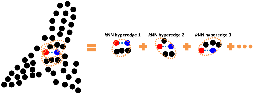
Figure 3: Intuitive illustration of $k$NN hypergraph construction. The left part shows a set of samples while the right part displays a collection of $k$NN hyperedges containing the two highlighted samples. Clearly, the $k$NN hyperedges encode the local neighboring information among data samples.

3) High-order over-clustering hypergraph. In practice, the vertices are often distributed in different cohesive vertex communities, and each community contains a set of mutually correlated vertices with some common properties. In order to effectively discover such cohesive vertex communities, we propose a high-order over-clustering hypergraph $G_{o}$ based on over-clustering (or over-segmentation) using different clustering methods. Specifically, an over-clustering mechanism is employed to generate a set of vertex groups, each of which corresponds to a cohesive vertex community (as shown in Fig. 2(a)). In this case, the vertices belonging to the same vertex community are mutually influenced, and work as the high-order contexts of the other vertices in the same vertex community, as illustrated in Fig. 4. Without loss of generality, we assume that there are $\mathcal{L}$ vertex communities in total. For convenience, let $E_{o}=\{e^{o}_{\ell}\}_{\ell=1}^{\mathcal{L}}$ denote these vertex communities, each of which corresponds to a hyperedge $e_{\ell}^{o}$. Based on these hyperedges, we define the high-order over-clustering hypergraph incidence matrix $H_{o}=(h_{o}(v_{i},e^{o}_{\ell}))_{|\mathbb{V}|\times\mathcal{L}}$ as:

$$h_{o}(v_{i},e^{o}_{\ell})=\frac{\sqrt{\mathbb{I}(v_{i},e_{\ell}^{o})(1+\frac{1}{|\mathfrak{N}_{i}^{\ell}|}\sum_{m\in\mathfrak{N}_{i}^{\ell}}a_{mi})}}{\sqrt{\underset{e^{o}_{\ell}\in E_{o}}{\sum}\mu_{\ell}\mathbb{I}(v_{i},e_{\ell}^{o})(1+\frac{1}{|\mathfrak{N}_{i}^{\ell}|}\sum_{m\in\mathfrak{N}_{i}^{\ell}}a_{mi})}},{}$$ (8)

where $\mathbb{I}(\cdot,\cdot)$ is the indicator function in Eq. (5), $\mathfrak{N}_{i}^{\ell}$ is the corresponding vertex index set of the nearest neighbors of $v_{i}$ in the hyperedge $e^{o}_{\ell}$ (s.t. $|\mathfrak{N}_{i}^{\ell}|=3$ in the experiments), and $\mu_{\ell}$ is the associated hyperedge weight of $e_{\ell}^{o}$ such that:

$$\mu_{\ell}=\frac{1}{2}\left(1+\frac{1}{|e^{o}_{\ell}|}\sum_{i\in\{q|v_{q}\in e^{o}_{\ell}\}}\sum_{m\in\mathfrak{N}_{i}^{\ell}}\frac{a_{mi}}{|\mathfrak{N}_{i}^{\ell}|}\right).{}$$ (9)

Here, $a_{mi}$ is the vertex-to-hyperedge similarity between $v_{i}$ and the $\ell$-th over-clustering hyperedge $e^{o}_{\ell}$. To ensure the robustness of similarity evaluation, we only take into account the affinity relationships between $v_{i}$ and its corresponding nearest neighbors (indexed by $\mathfrak{N}_{i}^{\ell}$) in $e^{o}_{\ell}$. Therefore, $a_{mi}$ is the similarity between $v_{i}$ and the $m$-th vertex of $\mathfrak{N}_{i}^{\ell}$. With the definition of $H_{o}$, the high-order over-clustering hypergraph similarity $c_{ij}$ between $v_{i}$ and $v_{j}$ is formulated as:

$$\begin{array}[]{ll}c_{ij}=\underset{e^{o}_{\ell}\in E_{o}}{\sum}\mu_{\ell}\hskip 1.42271pth_{o}(v_{i},e^{o}_{\ell})h_{o}(v_{j},e^{o}_{\ell})&{}\\ =\frac{\underset{e^{o}_{\ell}\in E_{o}}{\sum}\sqrt{\mu_{\ell}\mathbb{I}(v_{i},e_{\ell}^{o})\left(1+\frac{\sum_{m\in\mathfrak{N}_{i}^{\ell}}a_{mi}}{|\mathfrak{N}_{i}^{\ell}|}\right)}\sqrt{\mu_{\ell}\mathbb{I}(v_{j},e_{\ell}^{o})\left(1+\frac{\sum_{m\in\mathfrak{N}_{j}^{\ell}}a_{mj}}{|\mathfrak{N}_{j}^{\ell}|}\right)}}{\sqrt{\underset{e^{o}_{\ell}\in E_{o}}{\sum}\mu_{\ell}\mathbb{I}(v_{i},e_{\ell}^{o})\left(1+\frac{\sum_{m\in\mathfrak{N}_{i}^{\ell}}a_{mi}}{|\mathfrak{N}_{i}^{\ell}|}\right)}\sqrt{\underset{e^{o}_{\ell}\in E_{o}}{\sum}\mu_{\ell}\mathbb{I}(v_{j},e_{\ell}^{o})\left(1+\frac{\sum_{m\in\mathfrak{N}_{j}^{\ell}}a_{mj}}{|\mathfrak{N}_{j}^{\ell}|}\right)}}&{}\\ =\frac{\left<\mathbf{y}_{i},\mathbf{y}_{j}\right>}{\|\mathbf{y}_{i}\|\|\mathbf{y}_{j}\|},&\end{array}{}$$ (10)

where $\mathbf{y}_{q}$ is an $\mathcal{L}$-dimensional vector with the $\ell$-th element being $\sqrt{\mu_{\ell}\mathbb{I}(v_{q},e_{\ell}^{o})(1+\frac{1}{|\mathfrak{N}_{q}^{\ell}|}\sum_{m\in\mathfrak{N}_{q}^{\ell}}a_{mq})}$. Actually, $\mathbf{y}_{q}$ is a vertex-to-hyperedge feature vector, and its $\ell$-th element consists of two components: $\mu_{\ell}$ and $\mathbb{I}(v_{q},e_{\ell}^{o})(1+\frac{1}{|\mathfrak{N}_{q}^{\ell}|}\sum_{m\in\mathfrak{N}_{q}^{\ell}}a_{mq})$. As defined in Eq. (9), the left term measures the average cross-link degree of the within-community-$\ell$ vertices with respect to the other vertices in the same community, while the right term reflects the average affinity relationships between $v_{q}$ and the vertices in the $\ell$-th community. Therefore, the high-order over-clustering hypergraph similarity $c_{ij}$ can be viewed as the cosine similarity between two vertex-to-hyperedge feature vectors $\mathbf{y}_{i}$ and $\mathbf{y}_{j}$. As a result, a weighted similarity matrix $C=(c_{ij})_{N\times N}$ is obtained to capture the local grouping information on vertices. For simplicity, the high-order over-clustering hypergraph similarity matrix $C$ can be expressed as its corresponding matrix form: $C=H_{o}\Sigma_{o}H_{o}^{T}$, where $\Sigma_{o}$ is a diagonal matrix with the $\ell$-th diagonal element being $\mu_{\ell}$.

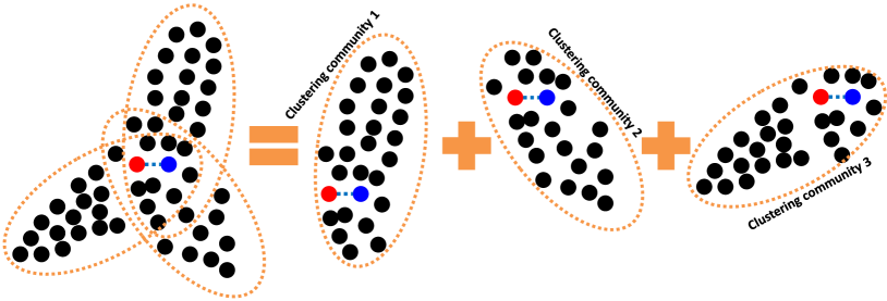
Figure 4: Intuitive illustration of high-order over-clustering hypergraph construction. The left part shows a set of samples while the right part displays a collection of high-order clustering hyperedges containing the two highlighted samples. Clearly, the high-order clustering hyperedges encodes the manifold structure information among data samples at larger scales.

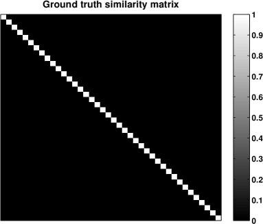
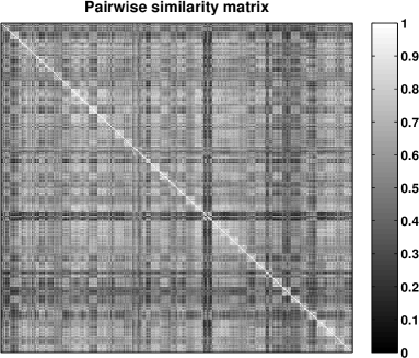
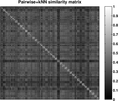
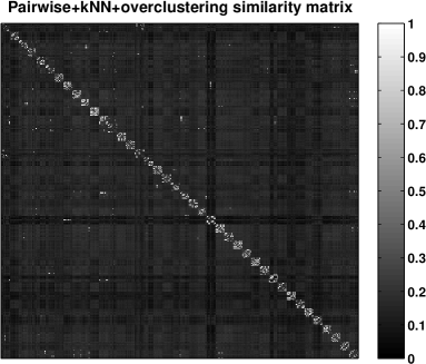
Figure 5: Illustration of different types of hypergraph similarity matrices. Specifically, the top-left subfigure shows the ground truth similarity matrix of the ORL face dataset (referred to in Sec. 3); the top-right subfigure displays the pairwise hypergraph similarity matrix; the bottom-left subfigure exhibits the pairwise+$k$NN hypergraph similarity matrix; the bottom-right subfigure draws our pairwise+$k$NN +over-clustering hypergraph similarity matrix. Clearly, our hypergraph similarity matrix is the closest to the ground truth.

Fig. 5 gives an example of showing the different hypergraph similarity matrices on the ORL face dataset (referred to in Sec. 3). By linearly combining the above three types of hypergraphs, a context-aware hypergraph similarity matrix $S=(s_{ij})_{N\times N}$ is obtained as follows:

$$S=\mathcal{H}\left(\begin{array}[]{ccc}\alpha\Sigma_{p}&\mathbf{0}&\mathbf{0}\\ \mathbf{0}&\beta\Sigma_{n}&\mathbf{0}\\ \mathbf{0}&\mathbf{0}&(1-\alpha-\beta)\Sigma_{o}\\ \end{array}\right)\mathcal{H}^{T},{}$$ (11)

where $\mathcal{H}=(H_{p}\thinspace H_{n}\thinspace H_{o})$ and $(\alpha,\beta)$ are the nonnegative weighting factors such that $(\alpha+\beta)\leq 1$. Encoding the local neighboring information, the $k$NN hypergraph plays a role in locally smoothing the clustering results (obtained by only using the pairwise hypergraph), as shown in the bottom-left part of Fig. 5. By constructing the high-order over-clustering hypergraph, we are capable of capturing the manifold structure information among data samples at larger scales, which leads to more accurate clustering results (shown in the bottom-right part of Fig. 5). Therefore, the final context-aware hypergraph similarity matrix keeps a balance among the three types of hypergraph information. In practice, it is easy to emphasize one particular type of hypergraph information by enlarging its associated weight. Fig. 2 (b) gives an example of illustrating the hypergraph clustering results based on the above hypergraph similarities.

2.2 Discriminative hypergraph partitioning for spectral clustering

Having defined a context aware vertex similarity measure, we now propose a discriminative hypergraph partitioning criterion based on this measure, with its corresponding optimization procedure.

1) Preliminaries of hypergraph partitioning. Hypergraph partitioning seeks an optimal hypergraph cut solution for effective data clustering. $\mathcal{K}$-way normalized cut [12] is a well-known hypergraph partitioning criterion, which aims to optimally partition the vertex set $\mathbb{V}$ into $\mathcal{K}$ disjoint subsets (i.e., $\mathbb{V}=\bigcup_{l=1}^{\mathcal{K}}\mathbb{V}_{l}$ s.t. $\mathbb{V}_{m}\bigcap\mathbb{V}_{n}=\emptyset$, $\forall m\neq n$) by solving the following optimization problem:

$$\begin{array}[]{cc}\mbox{\bf{max}}&f(X)=\frac{1}{\mathcal{K}}\sum_{n=1}^{\mathcal{K}}\frac{X_{n}^{T}SX_{n}}{X_{n}^{T}DX_{n}},{}\\ \mbox{\bf{s.t.}}&X\in\{0,1\}^{N\times\mathcal{K}},X\mathbf{1}_{\mathcal{K}}=\mathbf{1}_{N},\end{array}{}$$ (12)

where $X$ is an $N\times\mathcal{K}$ partition matrix such that $X^{T}X$ is a diagonal matrix, $\mathbf{1}_{d}$ denotes a $d\times 1$ vector with each element being 1, $D$ is an $N\times N$ diagonal matrix with the $m$-th diagonal element being the sum of the elements belonging to the $m$-th row of $S$ for $1\leq m\leq N$, and $X_{n}$ is the $n$-th column of $X$ for $1\leq n\leq\mathcal{K}$. As pointed out in [12], the optimization problem (12) is typically relaxed to:

$$\begin{array}[]{cl}\mbox{\bf{max}}&h(Z)=\frac{1}{\mathcal{K}}tr(Z^{T}SZ),{}\\ \mbox{\bf{s.t.}}&Z^{T}DZ=I_{\mathcal{K}},\end{array}{}$$ (13)

where $I_{\mathcal{K}}$ is a $\mathcal{K}\times\mathcal{K}$ identity matrix, $tr(\cdot)$ denotes the trace of a matrix, and $Z=X(X^{T}DX)^{-\frac{1}{2}}$. Eq. (13) is a trace maximization problem and can be solved by generalized eigenvalue decomposition. To simultaneously capture both intra-cluster compactness and the inter-cluster separability among the vertices in a unified clustering framework, we propose a discriminative hypergraph partitioning criterion which can be formulated as a trace-ratio optimization problem.

Input: A dataset $\mathbb{Z}=\{\mathbf{z}_{i}\}_{i=1}^{N}$ and the number of clusters $\mathcal{K}$

1. Obtain the hypergraph similarity matrix $S=(s_{ij})_{N\times N}$.

   • Compute the pairwise hypergraph similarity $u^{p}_{ij}$ in Eq. (3).

   • Obtain the $k$NN hypergraph similarity $u^{n}_{ij}$ in Eq. (7).

   • Compute the high-order over-clustering hypergraph

similarity $u^{c}_{ij}$ in Eq. (10).

Combine the above three similarities to generate $s_{ij}$ by Eq. (11).

Perform spectral graph partitioning.

• Compute the graph Laplacian matrix $Q=D-S$.

• Solve the optimization problem (19) by the Newton-Lanczos algorithm.

• Calculate a candidate graph partitioning solution $\widetilde{X}$ by: $\widetilde{X}=\mbox{Diag}(\mbox{diag}^{-\frac{1}{2}}({P}{P}^{T})){P}$.

• Iteratively refine $\widetilde{X}$ to find an optimal discrete solution $X$.

Output: The optimal graph partitioning solution $X$.

Algorithm 1 The proposed pairwise+$k$NN+over-clustering hypergraph spectral clustering algorithm (PKO+HSC).

2) Discriminative hypergraph partitioning criterion (DHPC). The proposed DHPC considers both the inter-cluster separability and the intra-cluster compactness, and thus aims to solve the following optimization problem:

$$\begin{array}[]{cl}\mbox{\bf{max}}&g(X)=\frac{1}{\mathcal{K}}\sum_{n=1}^{\mathcal{K}}\frac{X_{n}^{T}SX_{n}}{X_{n}^{T}QX_{n}}{}\\ &\hskip 22.76228pt=\frac{1}{\mathcal{K}}\sum_{n=1}^{\mathcal{K}}\frac{[X_{n}(X_{n}^{T}X_{n})^{-\frac{1}{2}}]^{T}S[X_{n}(X_{n}^{T}X_{n})^{-\frac{1}{2}}]}{[X_{n}(X_{n}^{T}X_{n})^{-\frac{1}{2}}]^{T}Q[X_{n}(X_{n}^{T}X_{n})^{-\frac{1}{2}}]},{}\\ \mbox{\bf{s.t.}}&X\in\{0,1\}^{N\times\mathcal{K}},X\mathbf{1}_{\mathcal{K}}=\mathbf{1}_{N},\end{array}{}$$ (14)

where $Q=D-S$. In the proposed DHPC, the intra-cluster compactness and the inter-cluster separability are respectively captured by $X_{n}^{T}SX_{n}$ and $X_{n}^{T}QX_{n}$, which are formulated as:

$$X_{n}^{T}SX_{n}=\sum_{i\in\mathbb{V}_{n}}\sum_{j\in\mathbb{V}_{n}}s_{ij},\hskip 5.69046ptX_{n}^{T}QX_{n}=\sum_{i\in\mathbb{V}_{n}}\sum_{j\notin\mathbb{V}_{n}}s_{ij},{}{}$$ (15)

where $\mathbb{V}_{n}$ denotes the vertex set belonging to the $n$-th cluster. The larger the value of $X_{n}^{T}SX_{n}$, the more compact the intra-cluster samples. The smaller the value of $X_{n}^{T}QX_{n}$, the more separable the inter-cluster samples. As a result, an optimal hypergraph partitioning solution is obtained by maximizing $g(X)$ in Eq. (14). For simplicity, let $P_{n}$ denote the vertex-to-cluster membership vector associated with the $n$-th cluster such that $P_{n}=X_{n}(X_{n}^{T}X_{n})^{-\frac{1}{2}}$, and $P$ denote the vertex-to-cluster membership matrix that is a concatenation of all the vertex-to-cluster membership vectors such that $P=(P_{1}\thinspace P_{2}\thinspace\ldots\thinspace P_{\mathcal{K}})=X(X^{T}X)^{-\frac{1}{2}}$. It can be shown that $P$ is an orthogonal matrix:

$$\begin{array}[]{cl}P^{T}P&=[X(X^{T}X)^{-\frac{1}{2}}]^{T}[X(X^{T}X)^{-\frac{1}{2}}]\\ &=(X^{T}X)^{-\frac{1}{2}}(X^{T}X)(X^{T}X)^{-\frac{1}{2}}=I_{\mathcal{K}},\end{array}{}$$ (16)

where $X^{T}X$ is a diagonal matrix. According to the conclusion in [12], we obtain $\widetilde{X}=\mbox{Diag}(\mbox{diag}^{-\frac{1}{2}}(PP^{T}))P$ that is the corresponding inverse transform of $P=X(X^{T}X)^{-\frac{1}{2}}$. Here, $\mbox{Diag}(\cdot)$ denotes a diagonal matrix formed from its vector argument, and $\mbox{diag}(\cdot)$ represents a column vector formed from the diagonal elements of its matrix argument. Consequently, the optimization problem in Eq. (14) can be rewritten as:

$$\begin{array}[]{cl}\mbox{\bf{max}}&g(X)=\frac{1}{\mathcal{K}}\sum_{n=1}^{\mathcal{K}}\frac{P_{n}^{T}SP_{n}}{P_{n}^{T}QP_{n}}=\frac{1}{\mathcal{K}}\sum_{n=1}^{\mathcal{K}}\frac{tr(P_{n}^{T}SP_{n})}{tr(P_{n}^{T}QP_{n})},\\ \mbox{\bf{s.t.}}&P^{T}P=I_{\mathcal{K}}.\end{array}{}$$ (17)

This is a trace-ratio-sum optimization problem, which is non-convex and difficult to solve [28]. Thus, we approximate the original optimization problem (17) using the following sum-trace-ratio optimization problem:

$$\begin{array}[]{cl}\mbox{\bf{max}}&f(P)=\frac{1}{\mathcal{K}}\frac{\sum_{n=1}^{\mathcal{K}}tr(P_{n}^{T}SP_{n})}{\sum_{n=1}^{\mathcal{K}}tr(P_{n}^{T}QP_{n})}=\frac{1}{\mathcal{K}}\frac{tr(\sum_{n=1}^{\mathcal{K}}P_{n}^{T}SP_{n})}{tr(\sum_{n=1}^{\mathcal{K}}P_{n}^{T}QP_{n})},\\ \mbox{\bf{s.t.}}&P^{T}P=I_{\mathcal{K}}.\end{array}{}$$ (18)

Due to $tr(\sum_{n=1}^{\mathcal{K}}P_{n}^{T}SP_{n})=tr(P^{T}SP)$ and $tr(\sum_{n=1}^{\mathcal{K}}P_{n}^{T}QP_{n})=tr(P^{T}QP)$, the above optimization problem (18) can be reformulated as:

$$\begin{array}[]{cl}\mbox{\bf{max}}&f(P)=\frac{1}{\mathcal{K}}\frac{tr(P^{T}SP)}{tr(P^{T}QP)},\\ \mbox{\bf{s.t.}}&P^{T}P=I_{\mathcal{K}}.\end{array}{}$$ (19)

The trace-ratio optimization problem (19) has been investigated in [29, 30, 33, 38]. In order to obtain an effective solution to Eq. (19), we therefore utilize the Newton-Lanczos algorithm [33] for trace-ratio maximization. The Newton-Lanczos algorithm includes the following three iterative steps:

• Compute the trace ratio $\rho=\frac{tr(P^{T}SP)}{tr(P^{T}QP)}$;

• Run the Lanczos algorithm [37] to compute the $\mathcal{K}$ largest eigenvalues of $S-\rho Q$ as well as their associated eigenvectors $(P_{1}\thinspace P_{2}\thinspace\ldots\thinspace P_{\mathcal{K}})\equiv P$;

• Repeat the above two steps until convergence.

In practice, the initial solution $P$ is chosen as the $\mathcal{K}$ principal eigenvectors (i.e., corresponding to the $\mathcal{K}$ largest eigenvalues) of the matrix $Q^{-1}S$. If $Q$ is a singular matrix, $Q^{-1}S$ is replaced with the matrix $(Q+\epsilon I_{N})^{-1}S$, where $I_{N}$ is an $N\times N$ identity matrix and $\epsilon$ is a small positive constant ($\epsilon=10^{-6}$ in the experiments).

Figure 6: Representative samples of the trajectory dataset. Each subfigure is associated with a representative sample from a particular trajectory cluster.

Figure 7: Representative samples of the Corel dataset. Each subfigure is associated with a representative sample from a particular image cluster.

After solving the trace-ratio optimization problem (19), we obtain a candidate solution $\widetilde{X}$ to Eq. (14) as follows:

$$\widetilde{X}=\mbox{Diag}(\mbox{diag}^{-\frac{1}{2}}(PP^{T}))P.{}$$ (20)

However, the candidate solution $\widetilde{X}$ is a real-valued hypergraph partitioning solution, and thus does not satisfy the discrete-solution requirements for data clustering. As a result, an iterative refining procedure [12] may be used to find the optimal discrete hypergraph partitioning solution $X$ to Eq. (14) (more details can be found in Steps four to eight of the algorithm in [12]). After combining the constructed pairwise+$k$NN+over-clustering hypergraphs (referred to in Sec. 2.1), we have a DHPC-based spectral clustering algorithm called PKO+HSC (pairwise+$k$NN+over-clustering hypergraph spectral clustering), as listed in Algorithm 1.

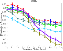
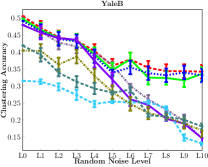
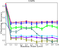
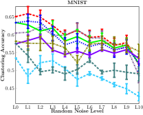
Figure 8: Clustering performances of the eight clustering algorithms regarding different random noise levels on the first four datasets. The first row corresponds to their clustering performances in NMI; and the second row is associated with their clustering performances in accuracy. The $(\alpha,\beta)$ configurations for weighting different types of hypergraphs on the four datasets are as follows: (ORL, YaleB.)$\rightarrow$(0.6, 0.2) and (USPS, MNIST)$\rightarrow$(0.4,0.4).

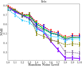
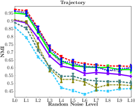
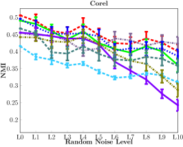
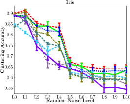
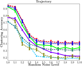
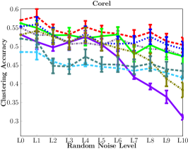
Figure 9: Clustering performances of the eight clustering algorithms regarding different random noise levels on the last three datasets. The first row corresponds to their clustering performances in NMI; and the second row is associated with their clustering performances in accuracy. The $(\alpha,\beta)$ configurations for weighting different types of hypergraphs on the three datasets are as follows: (Traj.)$\rightarrow$(0.6, 0.2) and (Iris, Corel)$\rightarrow$(0.4,0.4).

3 Experiments

3.1 Data description and implementation details

In the experiments, we evaluate the proposed PKO+HSC on seven datasets, which have the ground truth labels for classification and clustering tasks. The detailed configurations of these datasets are given as follows.

	ORL	YaleB	USPS	MNIST	Iris	Traj.	Corel
PKO+HSC	0.8529	0.6336	0.7918	0.5672	0.7981	0.9734	0.5061
PK+HSC	0.8159	0.6306	0.7334	0.4953	0.7648	0.9606	0.4540
PO+HSC	0.8111	0.6186	0.7348	0.5583	0.7793	0.9500	0.4907
PKO+NC	0.8164	0.6084	0.7815	0.5569	0.7878	0.9631	0.4958
CSC	0.8116	0.5849	0.7118	0.4882	0.7855	0.9031	0.4556
NRSC	0.7236	0.4718	0.5807	0.4328	0.7583	0.8587	0.4158
RWDSM	0.7891	0.5558	0.6741	0.4536	0.7869	0.9068	0.4423
STSC	0.7421	0.5295	0.4684	0.4368	0.7486	0.8882	0.4675
PKO+HSC	0.7300	0.5055	0.8409	0.6511	0.9000	0.9500	0.5700
PK+HSC	0.7057	0.4998	0.8043	0.6050	0.8957	0.9457	0.5497
PO+HSC	0.7074	0.4972	0.8093	0.6343	0.8899	0.9259	0.5619
PKO+NC	0.6883	0.4910	0.8241	0.6343	0.8833	0.9333	0.5533
CSC	0.6795	0.4796	0.7920	0.5746	0.8920	0.7720	0.5320
NRSC	0.6015	0.3154	0.6121	0.5348	0.8486	0.7126	0.4850
RWDSM	0.6669	0.4043	0.7686	0.5821	0.8976	0.7984	0.5312
STSC	0.6694	0.4187	0.4976	0.5759	0.8359	0.7173	0.5210

TABLE I: Clustering performances of the eight clustering algorithms in NMI and accuracy on the seven datasets without corruption. Specifically, the upper part corresponds to NMI; and the lower part is associated with accuracy. The $(\alpha,\beta)$ configurations for weighting different types of hypergraphs on the seven datasets are as follows: (ORL, YaleB, Traj.)$\rightarrow$(0.6, 0.2) and (USPS, MNIST, Iris, Corel)$\rightarrow$(0.4,0.4).

	(0.2, 0.2)	(0.2, 0.4)	(0.2, 0.6)	(0.4, 0.2)	(0.4, 0.4)	(0.6, 0.2)	(0.6, 0.4)	(0.2, 0.0)	(0.0, 0.2)
ORL	0.8182	0.8185	0.8229	0.8287	0.8350	0.8529	0.8251	0.8463	0.8359
YaleB	0.4730	0.5153	0.5690	0.5733	0.6189	0.6336	0.6227	0.4792	0.4668
USPS	0.7523	0.7648	0.7806	0.7779	0.7918	0.7631	0.7331	0.7059	0.7114
MNIST	0.5500	0.5595	0.5578	0.5561	0.5672	0.5543	0.5228	0.5600	0.5574
Iris	0.7961	0.7968	0.7971	0.7978	0.7981	0.7980	0.7777	0.7926	0.7958
Traj.	0.9548	0.9634	0.9638	0.9641	0.9638	0.9734	0.9631	0.9548	0.9668
Corel	0.4561	0.4772	0.4785	0.5033	0.5061	0.4626	0.4489	0.4561	0.4435
ORL	0.6775	0.6875	0.7000	0.7175	0.7075	0.7300	0.6950	0.7225	0.7050
YaleB	0.3271	0.3727	0.4209	0.4209	0.4450	0.5055	0.5044	0.3298	0.3271
USPS	0.8065	0.8323	0.8409	0.8301	0.8409	0.8194	0.8108	0.7677	0.7892
MNIST	0.6477	0.6479	0.6411	0.6344	0.6511	0.6500	0.6227	0.6244	0.6477
Iris	0.8903	0.8911	0.8942	0.8953	0.9000	0.8923	0.8900	0.8933	0.8967
Traj.	0.9401	0.9412	0.9422	0.9431	0.9437	0.9500	0.9400	0.9020	0.9220
Corel	0.5640	0.5600	0.5400	0.5660	0.5700	0.5580	0.5400	0.5340	0.5440

TABLE II: Clustering performances of the proposed PKO+HSC with different configurations of $(\alpha,\beta)$ in NMI and accuracy on the seven datasets without corruption. Specifically, the upper part corresponds to NMI; and the lower part is associated with accuracy.

The first dataset is the ORL face dataset. It comprises 400 face images of 40 persons, and each person has 10 images. The second dataset is a subset of the YaleB face dataset, and contains 2432 near frontal face images from 38 individuals under different illuminations. For computational convenience, all the face images from the two datasets are resized to $32\times 32$ pixels. The third dataset is a subset of the US Postal Service (USPS) handwritten digit dataset, and consists of 9298 $16\times 16$ handwritten digit images from ten clusters. The fourth dataset is a subset of the MNIST handwritten digit dataset, and constitutes 2000 $28\times 28$ digit images from ten clusters. As shown in Fig. 6, the fifth dataset [27] is a trajectory dataset containing 2500 trajectories from 50 clusters, and each cluster comprises 50 trajectories with complex shapes. The sixth dataset is the Iris dataset from the UCI repository, and contains 150 samples from 3 clusters. The seventh dataset is the Corel image dataset that is composed of 1000 images from ten clusters, as shown in Fig. 7.

For graph construction, the features used in the two face datasets and the two digit datasets are directly flattened into grayscale intensity column vectors. As a result, the feature dimensions for these four datasets are 1024 (ORL), 1024 (YaleB), 256 (USPS), and 784 (MNIST), respectively. In addition, the corresponding image features for the Corel dataset are the 960-dimensional GIST descriptors (as in [23]) that are widely used in computer vision and pattern recognition. The corresponding features for the trajectory dataset are 18-dimensional discrete Fourier transform (DFT) coefficient features (as in [24]). The feature dimension for the Iris dataset is 4, as shown in the UCI repository. Moreover, the kernel function $\mathcal{G}(\mathbf{z}_{i},\mathbf{z}_{j})$ (as in Eq. (3)) is selected as follows: $\mathcal{G}(\mathbf{z}_{i},\mathbf{z}_{j})=\exp\left(-\|\mathbf{z}_{i}-\mathbf{z}_{j}\|^{2}/2\sigma^{2}\right)$ where $\sigma$ is a scaling factor. In practice, $\sigma$ is tuned from the set $\{y|y=0.2\rho+(\lambda-1)0.2\rho\}$ where $\lambda$ is a positive integer such that $\lambda\in\{1,2,\ldots,15\}$ and $\rho$ is the average of the distances from each sample $\mathbf{z}_{i}$ to the other samples. The parameter $k$ in the $k$NN hypergraph is set to 3. The weighting factors $(\alpha,\beta)$ in Eq. (11) are chosen from the set $\{$(0.2, 0.2), (0.2, 0.4), (0.2, 0.6), (0.4, 0.2), (0.4, 0.4), (0.6, 0.2), (0.6, 0.4), (0.2, 0.0), (0.0, 0.2)$\}$. The task of constructing the high-order over-clustering hypergraph can be accomplished by using a set of existing clustering methods. In our case, we take advantage of classic spectral clustering [10] and multi-class spectral clustering [12] to generate a set of vertex communities. For each over-clustering method, the number of the vertex communities is chosen as $2\mathcal{K}$ with $\mathcal{K}$ being the desired number of clusters (referred to in Algorithm 1). Since we focus on the issues of iii) and iv) referred to in Sec. 1, $\mathcal{K}$ is directly set as the ground truth number of clusters for each dataset. The above experimental configurations remain the same for all the experiments below.

Computational complexity analysis Given $N$ data samples, our pairwise hypergraph construction requires $N^{2}$ kernel computation operations (referred to in Eq. (1)). Accordingly, the $k$NN hypergraph construction needs to calculate $N^{2}$ cosine similarities (defined in Eq. (7)) with respect to the $N$ data samples. Similarly, the over-clustering hypergraph construction involves $N^{2}$ cosine similarity computation operations (mentioned in Eq. (10)). The main computational cost of graph partitioning lies in the eigenvalue decomposition of $S-\rho Q$ while solving the optimization problem (19) using the Newton-Lanczos algorithm. According to [37], the time complexity of the Lanczos iterations in our graph partitioning is $\mathcal{O}(N^{2})$. Therefore, the overall time complexity of our method is $\mathcal{O}(N^{2})$, which is the same as standard spectral clustering methods. For example, the average running time of our method on the USPS dataset (s.t. $N=9298$) is 15.21 seconds. The spatial complexity of our method lies in the four aspects: 1) the $N\times N$ pairwise hypergraph incidence matrix $H_{p}$; 2) the $N\times N$ $k$NN hypergraph incidence matrix $H_{n}$; 3) the $N\times N$ over-clustering hypergraph incidence matrix $H_{o}$; and 4) the final $N\times N$ similarity matrix $S$. It therefore has $\mathcal{O}(N^{2})$ overall spatial complexity.

3.2 Competing algorithms

We compare the proposed PKO+HSC with several representative spectral clustering algorithms. These spectral clustering algorithms are recently proposed, and have significant impacts on the data clustering community. For descriptive convenience, they are respectively referred to as CSC (classic spectral clustering [10]), STSC (self-tuning spectral clustering [11]), and NRSC (noise-robust spectral clustering [15]).

In order to verify the effect of different hypergraph components, we compare the proposed PKO+HSC with PK+HSC (pairwise+$k$NN hypergraph spectral clustering) and PO+HSC (pairwise+over-clustering hypergraph spectral clustering). Actually, PK+HSC and PO+HSC are special cases of the proposed PKO+HSC with different configurations of $(\alpha,\beta)$. In order to evaluate the performance of different graph partitioning criteria, we perform a comparison experiment against PKO+NC (our context-aware hypergraph similarity measure together with the normalized cut criterion [12]). Furthermore, in order to demonstrate the effectiveness of our context-aware hypergraph similarity measure (defined in Eq. (11)), we make a quantitative comparison with another similarity measure called RWDSM (Random Walk Diffusion Similarity Measure [32]). We put both RWDSM and our similarity measure into the same discriminative hypergraph partitioning criterion (DHPC) for data clustering.

	ORL	YaleB	USPS	MNIST	Iris	Traj.	Corel
PKO+HSC	0.7626	0.5328	0.4966	0.5148	0.6003	0.7183	0.4496
PK+HSC	0.7266	0.4903	0.4834	0.4916	0.5212	0.7000	0.4302
PO+HSC	0.7370	0.5191	0.4052	0.5019	0.5844	0.6962	0.4300
PKO+NC	0.7453	0.5144	0.4819	0.4988	0.5856	0.7031	0.4349
CSC	0.6935	0.4634	0.1502	0.4589	0.4914	0.6596	0.3817
NRSC	0.6379	0.3853	0.1723	0.3798	0.5478	0.5544	0.3514
RWDSM	0.6493	0.4441	0.1308	0.4508	0.5373	0.6027	0.3955
STSC	0.6494	0.4315	0.3260	0.3944	0.5734	0.6099	0.3992
PKO+HSC	0.6107	0.3981	0.5527	0.6045	0.7485	0.5558	0.5391
PK+HSC	0.5614	0.3364	0.5321	0.5851	0.6849	0.5366	0.5102
PO+HSC	0.5725	0.3872	0.4624	0.5895	0.7333	0.4946	0.5177
PKO+NC	0.5884	0.3860	0.5348	0.5865	0.7306	0.5399	0.5212
CSC	0.4988	0.3229	0.2966	0.5592	0.6707	0.4067	0.4582
NRSC	0.4650	0.2471	0.3089	0.4866	0.6868	0.3237	0.4486
RWDSM	0.4558	0.2913	0.2545	0.5677	0.7049	0.3486	0.4897
STSC	0.5429	0.2845	0.3250	0.5107	0.6917	0.4089	0.4616

TABLE III: Clustering performances of the eight clustering algorithms in NMI and accuracy on the seven datasets by averaging different random noise levels. Specifically, the upper part corresponds to NMI; and the lower part is associated with accuracy. The $(\alpha,\beta)$ configurations for weighting different types of hypergraphs on the seven datasets are as follows: (ORL, YaleB, Traj.)$\rightarrow$(0.6, 0.2) and (USPS, MNIST, Iris, Corel)$\rightarrow$(0.4,0.4).

3.3 Evaluation criteria

For a quantitative comparison, we introduce two evaluation criteria—NMI (normalized mutual information) and clustering accuracy. Specifically, the NMI criterion is defined as: ${\rm NMI}(\mathbf{X},\mathbf{Y})=I(\mathbf{X},\mathbf{Y})/\sqrt{H(\mathbf{X})H(\mathbf{Y})}$ where $\mathbf{X}$ and $\mathbf{Y}$ are two random variables, $H(\mathbf{X})$ and $H(\mathbf{Y})$ are the corresponding entropies of $\mathbf{X}$ and $\mathbf{Y}$, and $I(\mathbf{X},\mathbf{Y})$ is the mutual information on $\mathbf{X}$ and $\mathbf{Y}$. In principle, $\mbox{NMI}(\mathbf{X},\mathbf{Y})$ has the range of $[0,1]$, and is equal to 1 when $\mathbf{X}=\mathbf{Y}$. As far as data clustering is concerned, the NMI criterion is explicitly formulated as:

$$\mbox{NMI}(\mathbf{S}^{\prime},\mathbf{S})=\frac{\sum_{i=1}^{\mathcal{C}}\sum_{j=1}^{K}\frac{q_{ij}}{m}\log\left(\frac{\frac{q_{ij}}{m}}{\frac{m_{i}}{m}\frac{m_{j}^{\prime}}{m}}\right)}{\sqrt{(\sum_{i=1}^{\mathcal{C}}\frac{m_{i}}{m}\log\frac{m_{i}}{m})(\sum_{j=1}^{K}\frac{m^{\prime}_{j}}{m}\log\frac{m^{\prime}_{j}}{m})}}{}$$ (21)

where $\mathbf{S}=\{S_{i}\}_{i=1}^{\mathcal{C}}$ is the ground truth clustering configuration of a dataset, $\mathbf{S}^{\prime}=\{S^{\prime}_{j}\}_{j=1}^{K}$ is the clustering configuration obtained by a clustering algorithm, $\mathcal{C}$ is the ground truth cluster number, $K$ is the obtained cluster number, $q_{ij}$ is the cardinality of the intersection of $S_{i}$ and $S^{\prime}_{j}$, $m_{i}$ is the cardinality of $S_{i}$, $m^{\prime}_{j}$ is the cardinality of $S^{\prime}_{j}$, and $m$ is the cardinality of the whole dataset. The larger the NMI, the better the clustering performance.

On the other hand, the clustering accuracy is defined as: $\mbox{Accuracy}=\frac{1}{m}\sum_{j=1}^{K}n_{j}$ where $n_{j}$ is the number of the samples whose ground truth cluster labels have the highest proportion in the $j$-th cluster $S^{\prime}_{j}$. The larger the clustering accuracy, the better the clustering results.

3.4 Clustering results

In the experiments, we aim to evaluate the clustering performances of different clustering algorithms in the following three aspects: i) evaluating the clustering performances (i.e., NMI and clustering accuracy) on the original datasets; ii) quantitative comparisons on the datasets after noise-based feature perturbations; and iii) performance evaluations on the datasets with outlier corruptions. The purposes of the above-mentioned three aspects are to verify the clustering effectiveness and the clustering robustness.

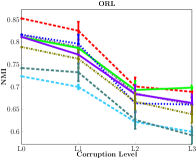
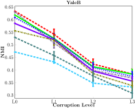
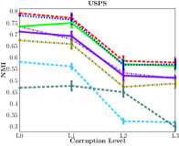
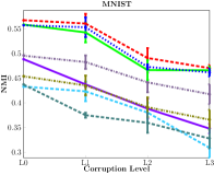
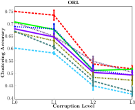
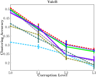
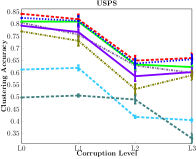
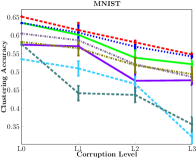
Figure 10: Clustering performances of the eight clustering algorithms regarding different outlier corruption levels on the first four datasets. The first row corresponds to their clustering performances in NMI; and the second row is associated with their clustering performances in accuracy. The $(\alpha,\beta)$ configurations for weighting different types of hypergraphs on the four datasets are as follows: (ORL, YaleB.)$\rightarrow$(0.6, 0.2) and (USPS, MNIST)$\rightarrow$(0.4,0.4).

For i), Tab. I reports the corresponding NMIs and accuracies of the eight clustering algorithms. It is seen from Tab. I that the proposed PKO+HSC obtains higher NMIs and accuracies than the other clustering algorithms. More specifically, the average NMI gains of PKO+HSC regarding the seven datasets are (5.53%, 3.65%, 2.26%, 8.07%, 20.78%, 11.16%, 19.67%) over those of (PK+HSC, PO+HSC, PKO+NC, CSC, NRSC, RWDSM, STSC), respectively; and the average accuracy gains are (2.83%, 2.42%, 2.80%, 9.02%, 25.55%, 10.72%, 21.58%), respectively. Furthermore, Tab. II reports the NMIs and accuracies of the proposed PKO+HSC with different configurations of the weighting factors $(\alpha,\beta)$. From Tab. II, we see that the clustering performances of the proposed PKO+HSC are not very sensitive to the configurations of the weighting factors.

For ii), noise-based feature perturbations are performed by using additive random noises. Figs. 8 and 9 show the NMI and accuracy curves with error bars in eleven different noise levels (i.e., $\mbox{L}_{0}$ corresponds to i), and $\mbox{L}_{1}\rightarrow\mbox{L}_{10}$ are associated with ten ascending noise levels whose magnitudes are chosen from $\{0.2,0.4,0.6,0.8,1.0,1.2,1.4,1.6,1.8,2.0\}$). Clearly, the proposed PKO+HSC achieves the highest NMIs and accuracies in most noise levels. Furthermore, Tab. III reports the average NMIs and accuracies of the eight clustering algorithms regarding different noise levels. The average NMI and accuracy gains of the proposed PKO+HSC are (6.03%, 5.19%, 2.80%, 23.54%, 34.54%, 26.92%, 20.43%) and (7.01%, 6.71%, 3.14%, 24.78%, 35.19%, 28.81%, 24.32%) over those of (PK+HSC, PO+HSC, PKO+NC, CSC, NRSC, RWDSM, STSC), respectively.

For iii), outlier corruptions are performed by randomly setting the feature elements to zeros. Fig. 10 displays the clustering performances of the eight clustering algorithms regarding four outlier corruption levels (i.e., $\mbox{L}_{0}$ corresponds to i), and $\mbox{L}_{1}\rightarrow\mbox{L}_{3}$ are associated with three ascending corruption levels whose corruption ratios are chosen from $\{0.2,0.4,0.6\}$). From Fig. 10, we see that the proposed PKO+HSC consistently achieves higher NMIs and accuracies than the other clustering algorithms. Moreover, Tab. IV shows the average NMIs and accuracies of the eight clustering algorithms regarding different outlier corruption levels. The average NMI and accuracy gains of the proposed PKO+HSC are (7.87%, 2.96%, 2.99%, 11.02%, 30.55%, 14.83%, 30.58%) and (7.39%, 3.80%, 2.91%, 10.11%, 34.62%, 14.04%, 33.66%) over those of (PK+HSC, PO+HSC, PKO+NC, CSC, NRSC, RWDSM, STSC), respectively.

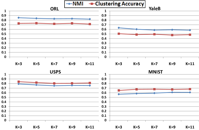
Figure 11: Clustering performances of the proposed PKO+HSC with different configurations of the nearest-neighbor number $k$ for $k$NN hypergraph construction in NMI and accuracy on the four datasets without corruption. The $(\alpha,\beta)$ configurations for weighting different types of hypergraphs on the four datasets are as follows: (ORL, YaleB.)$\rightarrow$(0.6, 0.2) and (USPS, MNIST)$\rightarrow$(0.4,0.4).

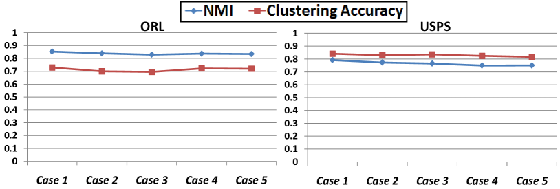
Figure 12: Clustering performances of the proposed PKO+HSC with different numbers of vertex communities (i.e., $\{2\mathcal{K},3\mathcal{K},4\mathcal{K},5\mathcal{K},6\mathcal{K}\}$ with $\mathcal{K}$ being the desired number of clusters) for high-order over-clustering hypergraph construction in NMI and accuracy on the two datasets without corruption. The $(\alpha,\beta)$ configurations for weighting different types of hypergraphs on the two datasets are as follows: ORL$\rightarrow$(0.6, 0.2) and USPS$\rightarrow$(0.4,0.4).

Besides, we report the clustering results of the proposed PKO+HSC with different configurations of the nearest-neighbor number $k$ for $k$NN hypergraph construction in Fig. 11. From Fig. 11, we see that the proposed PKO+HSC is not very sensitive to the settings of $k$. Moreover, Fig. 12 shows the clustering performances of the proposed PKO+HSC using different numbers of vertex communities for high-order over-clustering hypergraph construction in NMI and clustering accuracy on the two datasets. It is clearly seen from Fig. 12 that the proposed PKO+HSC is not very sensitive to the choice of the vertex community number.

Overall, the proposed PKO+HSC outperforms the other clustering algorithms. Considering three types of hypergraph information (i.e., pairwise, $k$NN, and over-clustering), the proposed PKO+HSC is capable of effectively exploring the intrinsic topological information among vertices. By optimizing the discriminative hypergraph partitioning criterion (DHPC), the proposed PKO+HSC considers both intra-cluster compactness and inter-cluster separability, resulting in the overall clustering robustness.

4 Conclusion and future work

In this work, we have proposed a context-aware hypergraph similarity measure (CAHSM), which is based on three types of hypergraphs—pairwise hypergraph, $k$-nearest-neighbor ($k$NN) hypergraph, and high-order over-clustering hypergraph. These hypergraphs capture the pairwise, neighborhood, and local grouping information on vertices. By effectively combining these types of affinity information, CAHSM is capable of effectively exploring the intrinsic structural information on vertices, resulting in the robust clustering performance. In order to fully capture the intra-cluster compactness and the inter-cluster separability of vertices, we have also designed a discriminative hypergraph partitioning criterion (DHPC) that is solved by trace-ratio maximization. Based on both CAHSM and DHPC, a robust spectral clustering algorithm (referred to as PKO+HSC) is developed for data clustering. Experimental results on various datasets, with and without noisy perturbation and outlier corruption, demonstrate that the proposed PKO+HSC has higher clustering robustness and effectiveness than competing algorithms in most cases.

On the other hand, this work is likely to have two limitations: 1) it is incapable of adaptively combining the aforementioned three types of hypergraphs; and 2) the number of clusters in spectral clustering is required to be provided in advance. Therefore, our future work is to figure out an adaptive weighting mechanism for hypergraph combination and an effective scheme for automatically estimating the cluster number prior to spectral clustering.

	PKO+HSC	PK+HSC	PO+HSC	PKO+NC	CSC	NRSC	RWDSM	STSC
ORL	0.7670	0.7376	0.7472	0.7341	0.7329	0.6612	0.7143	0.6731
YaleB	0.4959	0.4762	0.4852	0.4793	0.4642	0.3960	0.4496	0.4178
USPS	0.6814	0.6135	0.6548	0.6703	0.6093	0.4459	0.5726	0.4232
MNIST	0.5220	0.4591	0.5081	0.5110	0.4152	0.3862	0.4113	0.3747
ORL	0.6300	0.6019	0.6030	0.5933	0.5805	0.5093	0.5632	0.5418
YaleB	0.3701	0.3311	0.3597	0.3612	0.3346	0.2575	0.2946	0.3010
USPS	0.7420	0.6969	0.7183	0.7317	0.6861	0.5133	0.6549	0.4554
MNIST	0.5985	0.5497	0.5740	0.5883	0.5244	0.4585	0.5398	0.4529

TABLE IV: Clustering performances of the eight clustering algorithms by averaging different outlier corruption levels. Specifically, the upper part corresponds to NMI; and the lower part is associated with accuracy. The $(\alpha,\beta)$ configurations for weighting different types of hypergraphs on the four datasets are as follows: (ORL, YaleB.)$\rightarrow$(0.6, 0.2) and (USPS, MNIST)$\rightarrow$(0.4,0.4).

References

- [1] C. J. Alpert and A. B. Kahng, “Multiway Partitioning via Geometric Embeddings, Orderings and Dynamic Programming,” IEEE Trans. Computer-aided Design of Integrated Circuits and Systems, Vol.14, Iss.11, pp.1342-1358, 1995.
- [2] P. K. Chan, M. D. F. Schlag and J. Y. Zien, “Spectral K-Way Ratio-Cut Partitioning and Clustering,” IEEE Trans. Computer-aided Design of Integrated Circuits and Systems, Vol.13, Iss.9, pp.1088-1096, 1994.
- [3] B. Hendrickson and R. Leland, “An Improved Spectral Graph Partitioning Algorithm for Mapping Parallel Computations,” SIAM J. Sci. Comput., Vol.16, Iss.2, pp.452-459, 1995.
- [4] J. Shi and J. Malik, “Normalized Cuts and Image Segmentation,” IEEE Trans. Pattern Aanalysis Mach. Intelli., Vol.22, Iss.8, pp.888-905, 2000.
- [5] J. Malik, S. Belongie, T. Leung, and J. Shi, “Contour and Texture Analysis for Image Segmentation,” Int. J. Computer Vision, 2001.
- [6] Y. Weiss, “Segmentation Using Eigenvectors: A Unifying View,” in Proc. Int. Conf. Computer Vision, pp.975-982, 1999.
- [7] M. Meila and J. Shi, “Learning Segmentation by Random Walks,” Proc. Advances in Neural Information Processing Systems, pp.873-879, 2000.
- [8] Y. Gdalyahu, D. Weinshall and M. Werman, “Self-Organization in Vision: Stochastic Clustering for Image Segmentation, Perceptual Grouping, and Image Database Organization,” IEEE Trans. Pattern Analysis Mach. Intelli., Vol. 23, Iss. 10, pp.1053-1074, Oct. 2001.
- [9] C.H.Q. Ding, X. He, H. Zha, M. Gu and H.D. Simon, “A Min-Max Cut Algorithm for Graph Partitioning and Data Clustering,” in Proc. Int. Conf. Data Mining, pp.107-114, 2001.
- [10] A. Y. Ng, M. I. Jordan and Y. Weiss, “On Spectral Clustering: Analysis and An Algorithm,” Proc. Advances in Neural Information Processing Systems, MIT Press, 2001.
- [11] L. Zelnik-Manor and P. Perona, “Self-Tuning Spectral Clustering,” Proc. Advances in Neural Information Processing Systems, pp.1601-1608, 2005.
- [12] S.X. Yu and J. Shi, “Multiclass Spectral Clustering,” in Proc. Int. Conf. Computer Vision, Vol.1, pp.313-319, 2003.
- [13] B. Nadler, S. Lafon, R. Coifman, and I. Kevrekidis, “Diffusion Maps, Spectral Clustering and Eigenfunctions of Fokkerplanck Operators,” Proc. Advances in Neural Information Processing Systems, pp.955-962, 2006.
- [14] H. Chang and D. Y. Yeung, “Robust Path-Based Spectral Clustering with Application to Image Segmentation,” in Proc. Int. Conf. Computer Vision, 2005.
- [15] Z. Li, J. Liu, S. Chen, and X. Tang, “Noise Robust Spectral Clustering,” in Proc. Int. Conf. Computer Vision, 2007.
- [16] U. Von Luxburg, “A Tutorial on Spectral Clustering,” Statistics and Computing, Vol. 17, Iss. 4, pp. 395-416, 2007.
- [17] D. Zhou, J. Huang, and B. Schökopf, “Learning With Hypergraphs: Clustering, Classification, and Embedding,” in Proc. Advances in Neural Information Processing Systems, 2006.
- [18] S. Agarwal, J. Lim, L. Zelnik Manor, P. Perona, D. Kriegman, and S. Belongie, “Beyond Pairwise Clustering,” in Proc. IEEE Conf. Computer Vision Pattern Recognition, 2005.
- [19] R. Zass and A. Shashua, “Probabilistic Graph and Hypergraph Matching,” in Proc. IEEE Conf. Computer Vision Pattern Recognition, 2008.
- [20] L. Sun, S. Ji, and J. Ye, “Hypergraph Spectral Learning for Multi-Label Classification,” in Proc. ACM SIG KDD, 2008.
- [21] Y. Huang, Q. Liu, and D. Metaxas, “Video Object Segmentation by Hypergraph Cut,” in Proc. IEEE Conf. Computer Vision Pattern Recognition, 2009.
- [22] Y. Huang, Q. Liu, S. Zhang, and D. N. Metaxas, “Image Retrieval via Probabilistic Hypergraph Ranking,” in Proc. IEEE Conf. Computer Vision Pattern Recognition, 2010.
- [23] A. Oliva and A. Torralba, “Modeling The Shape of The Scene: A Holistic Representation of The Spatial Envelope,” Int. J. Computer Vision, 42(3):145-175, 2001.
- [24] A. Naftel and S. Khalid, “Motion Trajectory Learning in the DFT-Coefficient Feature Space,” in Proc. IEEE Int. Conf. Computer Vision Systems, 2006.
- [25] F. Lauer and C. Schnörr, “Spectral Clustering of Linear Subspaces for Motion Segmentation,”, in Proc. Int. Conf. Computer Vision, 2009.
- [26] W. Hu, D. Xie, Z. Fu, W. Zeng, and S. Maybank, “Semantic-Based Surveillance Video Retrieval,” IEEE Trans. on Image Processing, Vol. 16, Iss. 4, pp. 1168-1181, 2007.
- [27] J. Hsieh, S. Yu, and Y. Chen, “Motion-Based Video Retrieval by Trajectory Matching,” IEEE Trans. on Circuit System for Video Technology, Vol. 16, Iss. 3, pp. 396-409, 2006.
- [28] P. Wang, C. Shen, H. Zheng, and Z. Ren, “A Variant of the Trace Quotient Formulation for Dimensionality Reduction,” pp. 277-286, in Proc. Asian Conf. Computer Vision, 2009.
- [29] H. Wang, S. Yan, D. Xu, X. Tang, and T. Huang, Trace Ratio vs. Ratio Trace for Dimensionality Reduction, in Proc. IEEE Conf. Computer Vision Pattern Recognition, 2007.
- [30] Y. Jia, F. Nie, and C. Zhang, Trace Ratio Problem Revisited, IEEE. Trans. on Neural Networks, Vol. 20, Iss. 4 pp. 729-735, 2009.
- [31] Z. Lu and M.A. Carreira-Perpiñán, “Constrained Spectral Clustering through Affinity Propagation,” in Proc. IEEE Conf. Computer Vision Pattern Recognition, 2008.
- [32] X. Li, W. Hu, Z. Zhang, and Y. Liu, “Spectral Graph Partitioning Based on a Random Walk Diffusion Similarity Measure,” in Proc. Asian Conf. Computer Vision, 2009.
- [33] T. T. Ngo, M. Bellalij, and Y. Saad, “The Trace Ratio Optimization Problem,” SIAM Review, Vol. 54, Iss. 3, pp. 545-569, 2012.
- [34] Y. Yang, Y. Yang, Y. Zhang, X. Du, H. T. Shen, and X. Zhou, “Discriminative Nonnegative Spectral Clustering with Out-of-Sample Extension,” IEEE Trans. Knowledge and Data Engineering, 2012.
- [35] F. Wang, C. Zhang, T. Li, “Clustering with Local and Global Regularization,” IEEE Trans. Knowledge and Data Engineering, Vol. 21, Iss. 12, pp. 1665-1678, 2009.
- [36] D. Cai, X. He, and J. Han, “Spectral Regression for Efficient Regularized Subspace Learning,” in Proc. Int. Conf. Computer Vision, 2007.
- [37] http://en.wikipedia.org/wiki/Lanczos_algorithm
- [38] C. Shen, H. Li, and B. J. Michael, “Supervised Dimensionality Reduction via Sequential Semidefinite Programming,” Pattern Recognition, Vol. 41, Iss. 12, pp. 3644-3652, 2008.