Adjusting models of ordered multinomial outcomes for nonignorable nonresponse in the occupational employment statistics survey

Abstract

An establishment’s average wage, computed from administrative wage data, has been found to be related to occupational wages. These occupational wages are a primary outcome variable for the Bureau of Labor Statistics Occupational Employment Statistics survey. Motivated by the fact that nonresponse in this survey is associated with average wage even after accounting for other establishment characteristics, we propose a method that uses the administrative data for imputing missing occupational wage values due to nonresponse. This imputation is complicated by the structure of the data. Since occupational wage data is collected in the form of counts of employees in predefined wage ranges for each occupation, weighting approaches to deal with nonresponse do not adequately adjust the estimates for certain domains of estimation. To preserve the current data structure, we propose a method to impute each missing establishment’s wage interval count data as an ordered multinomial random variable using a separate survival model for each occupation. Each model incorporates known auxiliary information for each establishment associated with the distribution of the occupational wage data, including geographic and industry characteristics. This flexible model allows the baseline hazard to vary by occupation while allowing predictors to adjust the probabilities of an employee’s salary falling within the specified ranges. An empirical study and simulation results suggest that the method imputes missing OES wages that are associated with the average wage of the establishment in a way that more closely resembles the observed association.

copyrightownerIn the Public Domain

, and

t1Funded by the American Statistical Association, National Science Foundation and Bureau of Labor Statistics (ASA/NSF/BLS) Fellowship program during the period 2011–2013.

1 Introduction

Every large survey has to contend with nonresponding units. Estimates are commonly adjusted by rescaling each unit’s sample weight proportionally to the inverse of its response probability. Response probabilities are modeled conditionally on available auxiliary information [see, e.g., Kim and Kim (2007)]. For example, the linear estimator $\sum_{i\in S}w_{i}\mathbf{Y}_{i}$ for a population parameter based on the dependent variable $\mathbf{Y}_{i}$ using data from the sample $S$ would be adjusted as

$$\sum_{i\in S_{R}}p(\mathbf{x}_{i})^{-1}w_{i}\mathbf{Y}_{i},$$

where $\{w_{i}\}_{i=1}^{N}$ is a set of predefined fixed sample weights, $S_{R}$ is the subset of responding units in the sample, and $p(\mathbf{x}_{i})$ is the estimated probability of unit $i$ responding given the auxiliary information $X_{i}=x_{i}$.

There are a number of methods for adjusting the weights. These include using weighting classes [Little (1982)], post-stratification [Holt and Smith (1979)], calibration [Kott (2006)] and nearest neighbor approaches [Chen and Shao (2000)]. All of the weight adjustment methods aim to account for missing data of the nonrespondents by scaling up the data of responding units. Therefore, these weighting adjustments implicitly impute missing data as a linear combination of the observed data.

Weight adjustments can reduce bias introduced due to the missing information if the auxiliary variables used to calculate nonresponse probabilities are predictive of nonresponse. The adjustments can even reduce the mean squared error of an estimator if these variables are also associated with the outcome variable [Little and Vartivarian (2005)]. Adjusted estimators will be unbiased if the nonresponse mechanism is missing at random (MAR) given the auxiliary information and the response propensity model is correctly specified [Rubin (1976); Little and Rubin (2002)].

However, when the probability of response is associated with outcome variables even after conditioning on all auxiliary variables, the estimator could still be biased even after adjusting the weights for nonresponse. For example, Schenker et al. (2011) report on a study of bone mineral density using scan data, where most of the missing data was a direct result of a subject’s characteristics such as body mass index (BMI) and age. In fact, subjects over a certain age or with a BMI over a specific limit were excluded from the scan (by medical necessity). Therefore, all observed scan data came from younger subjects and/or subjects with lower BMI compared to some subjects with unobserved data. Since these characteristics are also highly associated with the outcome variable (bone mineral density), adjustment for this type of missingness requires a unverifiable model (explicitly or implicitly) to extrapolate from the observed data [Chang and Kott (2008); Kott and Chang (2010)].

In this article, we propose to adjust the occupational wage data from the Bureau of Labor Statistics (BLS) Occupational Employment Statistics survey (OES) using auxiliary variables obtained from administrative data to reduce bias due to unit nonresponse. Among the available variables is the average wage per employee for each establishment. Phipps and Toth (2012) demonstrated that this average wage tended to be lower for responding establishments than for nonrespondents, even after conditioning on the other auxiliary variables. In addition, the work of Groshen (1991) and Lane, Salmon and Spletzer (2007) suggests an establishment’s average wage is highly associated with occupational wages at that establishment.

Adjusting the occupational wage data for nonresponse is complicated by the structure of the data. The OES collects total counts of employees at each establishment in twelve predefined ordered wage ranges for each occupation. By collecting the wage interval data in this manner the OES data yield quantile estimates of wages for each occupation as well as averages. Thus, this data structure has more utility than aggregated totals of employment and wages, but adjusting for missing values becomes more difficult.

Indeed, if only mean wages were collected, the data could be adjusted using one of the weighting methods enumerated previously. However, due to the structure of the data and because there are certain domains for which occupational wages estimates are produced that contain nonresponding units with a higher establishment-level average wage per employee than all responding units, we argue that any weighting approach to adjust for nonresponse will lead to biased domain estimates.

To preserve the current data structure, we propose a method to impute each missing establishment’s wage interval count data as an ordered multinomial random variable, using a separate survival model for each occupation. Each model incorporates known auxiliary information associated with the distribution of the occupational wage data. Section 2 introduces the OES survey data, which provides the motivation for the proposed model-based method of adjustment. Section 3 describes the new method and explains how it incorporates the administrative data. Section 4 compares the imputed data produced using the new procedure with the existing method used by the OES and includes results of a simulation study. The code and data sets for these models are available at the Bureau of Labor Statistics through the external research program.

2 The OES occupational wage data

The BLS Occupational Employment Statistics (OES) survey, an establishment survey, measures occupational employment and wage rates for around 800 occupations in the Standard Occupational Classification (SOC) system by industry for states and territories in the United States. Estimates are produced at the national, state and metropolitan statistical area levels using data from approximately 1.2 million sampled establishments.

The sample is drawn from the Quarterly Census of Employment and Wages (QCEW), a frame of about 9 million establishments across all nonfarm industries. The frame contains administrative data on a number of variables for every establishment, including total employment for each of the three months in the quarter; total wages paid during that quarter ($\mathsf{WAGE}$); data-defined groups of industries ($\mathsf{IND}$) defined by the six digit North American Industry Classification System (NAICS) code; the metropolitan or nonmetropolitan area where the establishment is located ($\mathsf{MSA}$), an indicator of whether the MSA is in the largest of six size categories ($\mathsf{MSACATT6}$), and whether or not the establishment is part of a national multi-establishment firm ($\mathsf{MULTI}$). The average quarterly wage per employee,

$$\mathsf{AVEWAGE}=\mathsf{WAGE}/\mathsf{EMPL},$$ (1)

is calculated for every establishment (including nonrespondents) using the frame data. The variable $\mathsf{EMPL}$ is the average reported employment over the three months in the quarter. The establishments are sampled using a probability proportional to size (p.p.s.) design that is stratified by industry and area.

A responding establishment reports wages for the OES survey by occupational code. The data is reported by the establishment $i$ by listing the number of employees with a given occupational code that have hourly wages contained in a given interval $I_{l}=[a_{l},b_{l}]$, for each of twelve wage intervals $l=1,\ldots,12$. Table 1 illustrates the tabular form of the occupational data collected by the OES for an establishment.

Table 1: Example of the data collected for OES occupational wage survey from establishment $i$. The number of employees $e_{icl}$, with SOC code $c=1,\ldots,C_{i}$, that have an hourly wage contained in interval $I_{l}=[a_{l},b_{l}]$, for $l=1,\ldots,12$, is collected for each of the $C_{i}$ occupations represented at establishment $i$. The twelve wage intervals are the same for every occupation code, but vary across states (these differences are limited to the first two wage intervals and are driven by the state’s minimum wage). For example, the November 2006 panel, the lower bound of hourly-wage interval one, $a_{1}$, ranges by state from $6.35 to $8.42 per hour, while the lower bound of the second interval, $a_{2}$, ranges from $8.42 to $10.61 per hour. The last wage interval $I_{12}$ is open, $[a_{12},\infty)$. These wage intervals are regularly adjusted for inflation, so they change over time

SOC	$\bolds{I_{1}}$	$\bolds{I_{2}}$	$\bolds{I_{3}}$	$\bolds{I_{4}}$	$\bolds{I_{5}}$	$\bolds{I_{6}}$	$\bolds{I_{7}}$	$\bolds{I_{8}}$	$\bolds{I_{9}}$	$\bolds{I_{10}}$	$\bolds{I_{11}}$	$\bolds{I_{12}}$
1	$e_{i11}$	$e_{i12}$	$e_{i13}$	$e_{i14}$	$e_{i15}$	$e_{i16}$	$e_{i17}$	$e_{i18}$	$e_{i19}$	$e_{i110}$	$e_{i111}$	$e_{i112}$
2	$e_{i21}$	$e_{i22}$	$e_{i23}$	$e_{i24}$	$e_{i25}$	$e_{i26}$	$e_{i27}$	$e_{i28}$	$e_{i29}$	$e_{i210}$	$e_{i211}$	$e_{i212}$
⋮						⋮						⋮
$c$	$e_{ic1}$	$e_{ic2}$	$e_{ic3}$	$e_{ic4}$	$e_{ic5}$	$e_{ic6}$	$e_{ic7}$	$e_{ic8}$	$e_{ic9}$	$e_{ic10}$	$e_{ic11}$	$e_{ic12}$
⋮						⋮						⋮
$C_{i}$	$e_{iC_{i}1}$	$e_{iC_{i}2}$	$e_{iC_{i}3}$	$e_{iC_{i}4}$	$e_{iC_{i}5}$	$e_{iA_{i}6}$	$e_{iA_{i}7}$	$e_{iC_{i}8}$	$e_{iC_{i}9}$	$e_{iC_{i}10}$	$e_{iC_{i}11}$	$e_{iC_{i}12}$

This wage interval data is used to produces estimates of the total employment, mean wage, mean salary, as well as estimates for the hourly and annual 10th, 25th, 50th, 75th and 90th percentile wages for every occupation. Details on how these estimates are computed using interval data are presented in Piccone and Hesley (2010). OES also publishes a mean relative standard error for the total employment and mean wage estimates. In order to retain the same level of utility of the OES data, any imputation procedure must produce counts for each of twelve wage intervals.

3 Imputing ordered multinomial wage data

Though the OES achieves a high overall response rate (78%, one of the highest of any BLS establishment survey), bias in the estimates due to nonresponse could still be a problem. This is particularly true in smaller subdomains if the estimates are not properly adjusted. Currently the OES uses a nearest-neighbor type imputation procedure to account for missing occupational wage data due to nonresponse. For each nonresponding establishment, the list of occupations to impute, as well as the proportion of employees in each occupation, is taken from a donor establishment selected from a group of identified neighbors based on industry and location. The missing wage interval data is then imputed by taking an average of all nearby responding units’ data, where neighboring establishments are identified based on geography, industry, size and ownership status. More details regarding the imputation and estimation procedures can be found in the OES State Operations Manual [Bureau of Labor Statistics (2011)].

The current method adjusts for unit nonresponse by replacing the missing unit’s data with an average of the data from responding establishments that are similar to the nonresponding unit. However, when all the responding units in a neighborhood have smaller values of $\mathsf{AVEWAGE}$ than a nonresponding unit, weighting-up wage data of the responding units will not adequately account for the missing wage data for occupations that are associated with the $\mathsf{AVEWAGE}$ of an establishment. For example, Table 2 gives a hypothetical example (similar to situations confronted by the OES) of five establishments’ wage data for a given occupation in the form collected by OES. Three of the establishments responded, while two establishments did not respond.

Table 2: Hypothetical example of occupational wage data for five establishments in a given domain defined by industry and geographic area. Each row gives the establishment’s id, total number of employees with the given occupational code, counts of the number of employees in each of the twelve wage intervals, the average wage per employee $\mathsf{AVEWAGE}$, and the response indicator, where $R=1$ means that the establishment responded to the OES survey. The wage interval counts are not observed (italicized) for the two establishments with $R=0$. In this example, only five establishments employ workers with this occupational code in this industry and area, and the two establishments with the highest $\mathsf{AVEWAGE}$ (establishments 2 and 4) did not respond to the survey

id	tot	1	2	3	4	5	6	7	8	9	10	11	12	AVEWAGE	$\bolds{R}$
1	08	0	0	0	0	0	1	3	1	2	1	0	0	15,981	1
2	10	0	0	0	0	0	0	0	1	2	2	1	4	23,364	0
3	04	0	0	0	0	1	2	0	0	0	1	0	0	0,8420	1
4	07	0	0	0	0	0	0	0	0	1	1	3	2	27,343	0
5	08	0	0	0	0	0	0	2	0	4	2	0	0	15,058	1

In this example, no weight-based method will work using these establishments because replacing either of the missing establishments’ data with any linear combination of the responding establishments’ data will lead to inflated cell counts at the lower level of wage categories and have cell counts of zero at the highest wage categories. This is not representative of the nonresponding establishments’ data. Any method for adjusting for nonresponse should be able to adequately adjust the shape of the induced empirical cumulative distribution function (ECDF).

Figure 1: Empirical cumulative distribution function (CDF) for customer service representatives (top) and general managers (bottom) stratified by tertiles of $\mathsf{AVEWAGE}$. The wage of an employees at an establishment in the highest tertile of $\mathsf{AVEWAGE}$ (dotted line) is more likely to fall in a higher wage interval than that of an employee at an establishment in a lower tertile (middle${}={}$dashed, lowest${}={}$solid). This is shown to be true for both the lower wage earning occupation, customer service representatives, as well as the higher wage earning occupation, general managers.

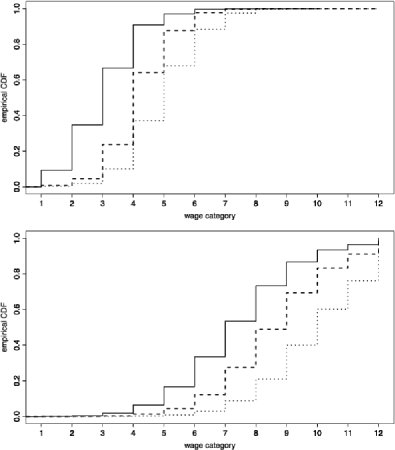
To illustrate, consider the distribution of wage categories from respondents for two common occupations: customer service representatives and general managers. Figure 1 displays the ECDF for the 12 wage categories using all observed data from establishments reporting on customer service representatives (top) and from establishments reporting on general managers (bottom) stratified by tertiles of the average wage distribution ($\mathsf{AVEWAGE}$) computed from the frame data. An employee’s wage at an establishment in the highest tertile of $\mathsf{AVEWAGE}$ is more likely to fall in a higher wage interval than that of an employee at an establishment in a lower tertile. Note that the overall distribution is shifted to the right in comparison with the customer service representatives, with higher average wages for general managers reflecting the generally higher pay for this occupation.

We propose a method that extrapolates from $\mathsf{AVEWAGE}$ of each establishment, as well as incorporates other important establishment characteristics using a model of the ECDF. The proposed model of the probability that an individual employee (in that establishment for a given occupation) falls in each of the 12 wage categories is modeled as a flexible “time-to-event” (survival) model. We then sample from the resulting distribution to impute missing OES occupational wage values.

We use a Cox proportional hazards regression for discrete failure times to model this wage distribution [Cox (1972)]. For a given establishment with characteristic variables $\mathbf{X}$, let $I$ be the interval in which the employee’s salary falls for $I=\{1,\ldots,12\}$. The model for the hazard is given by

$$\lambda(l)=\frac{P(L=l)}{P(L\geq l)}=\lambda_{0}(l)\exp{\bolds{\beta}^{\prime}\mathbf{X}},$$ (2)

where $\lambda_{0}(l)$ is the baseline hazard function,

$$\beta^{\prime} = (\beta_{0},\beta_{1},\ldots,\beta_{9}),$$

$$\mathbf{X}^{\prime} = {\bigl{(}1,\mathbf{X}_{1},\mathbf{X}_{1}^{2},\mathbf{X}_{2},\mathbf{X}_{2}^{2},\mathbf{X}_{3},\mathbf{X}_{1}\mathbf{X}_{3},\mathbf{X}_{4},\mathbf{X}_{5},\mathbf{X}_{6}\bigr{)}},$$

where $\mathbf{X}_{1}=\mathsf{AVEWAGE}$, $\mathbf{X}_{2}=\log(\mathsf{EMPL})$, $\mathbf{X}_{3}=\mathsf{SINGLE}$, $\mathbf{X}_{4}=\mathsf{MSACATT6}$, $\mathbf{X}_{5}=\mathsf{BMSA}$, and $\mathbf{X}_{6}=\mathsf{MULTI}$.

Since there are no censored outcomes, all employees must end up in one of the 12 wage categories. The Efron (1977) estimator is used to account for ties, since there are only twelve possible intervals. Therneau (2013) states that this approximation is more accurate than the Breslow when dealing with tied death times as well as computationally efficient. Use of the exact conditional likelihood is not computationally tractable for this example.

Quadratic terms are included for $\mathsf{AVEWAGE}$ and $\log(\mathsf{EMPL})$ to account for the quadratic relationship between these variables and occupational wages. We also adjust the establishments employing only a single employee within a given occupation differently, because the relationship between the occupational wage and $\mathsf{AVEWAGE}$ was observed to be different than establishments with multiple employees within that occupation. Likewise, the occupational wages of employees of establishments located in large MSAs had a different relationship to $\mathsf{AVEWAGE}$ than those in smaller MSAs. Therefore, we added two occupation specific variables $\mathsf{SINGLE}$ and $\mathsf{BMSA}$. The variable $\mathsf{SINGLE}=1$, if the establishment has only a single employee in that occupation and $\mathsf{BMSA}$ is an identifier of any MSAs where there are many ($\geq$250) establishments employing people in the given occupation (see Appendix for details on handling MSAs).

The baseline hazard function $\lambda_{0}(t)$ is a data-driven occupation specific step function, which can jump at each of the wage categories $t$. This is estimated using the empirical distribution of wage category counts. The model is stratified on classes defined using $\mathsf{IND}$ so that a different baseline hazard function $\lambda_{0}(t)$ is estimated for each industry class (see Appendix for details on how the industry classes are defined). We fit the model using the survival package in R [Therneau (2013)], accounting for clustering within each establishment.

Given the establishment-level variables for a nonresponding establishment, the survival model parameter estimates can be used to generate predicted probabilities that an employee with the given occupation falls into each of the 12 possible wage categories. We impute the missing data for the establishment by taking a random draw from a multinomial distribution with those probabilities for each employee at the establishment within that occupation.

This approach is attractive because the model for the hazard of falling into a lower wage category can extrapolate on average wage while including the other establishment-level characteristics in the imputation process. Due to the model’s flexibility, it allows the occupation specific baseline hazard (of falling into a lower wage category) to be unspecified, with predictors controlling the shape within the constraints of the model.

Currently, the OES uses a jackknife procedure to estimate sampling error, with additional variance components due to the categorization of wage data. In order to account for variability due to imputation, imputations could be resampled within each jackknife replication pool.

4 Evaluating the proposed imputation method

One difficulty with assessing nonresponse adjustment methods and their impact on a real survey is that the true missing values are unknown. In this section we attempt to evaluate the proposed imputation procedure by comparing the imputed values to observed values, considering the impact of the adjustment on estimates like those produced by the OES, as well as testing the procedure using a simulation with known response probabilities.

4.1 Comparison with existing OES imputation procedure

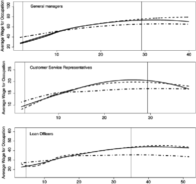
We start by comparing the relationship of the imputed values and the predictor variables to that of the observed values. Obviously, if the missing values are due to nonignorable nonresponse, there is no reason the imputed values should have the same relationship to predictor variables as the observed values, but it would seem desirable all the same [Abayomi, Gelman and Levy (2008)]. Figure 2 displays the predicted relationship between the occupational mean wage and $\mathsf{AVEWAGE}$ for general managers, customer service representatives and loan officers. The dashed line indicates the observed relationship between $\mathsf{AVEWAGE}$ and wage within an occupation for the respondents, while the solid line represents imputations using the proposed method and the dash-dot line represents imputations using the existing OES method over $\mathsf{AVEWAGE}$. All three lines are smoothed estimates of the functional relationship among occupational wage and the variable $\mathsf{AVEWAGE}$. The wage curves demonstrate an increasing relationship with respect to $\mathsf{AVEWAGE}$. Also, the proposed new method (solid line) more closely parallels the relationship between $\mathsf{AVEWAGE}$ and the observed wage for that occupation when compared to the existing OES imputation method (dash-dot line) for all three occupations shown here. This was the case for all occupations tested in an empirical study.

Figure 2: Average occupational wage for each establishment computed using imputed values from the new and current imputation methods compared to the observed data. The y-axis gives the average occupational wage for each establishment computed using imputed data from the new method (solid line), imputed data from the current OES method (dash-dot line) and the observed wage data (dashed line). The three average occupational wages are plotted over the average overall wage for each establishment, $\mathsf{AVEWAGE}$, computed from the administrative record data. The computed occupational average wages are displayed for three occupations: general managers (top), customer service representatives (middle) and loan officers (bottom). The comparisons show that the occupational average wages computed using the imputed data from the new method match the observed average wages more closely than the average wages using the imputed data from the old method. The two vertical lines indicate the location of the 2.5th and the 97.5th percentiles of $\mathsf{AVEWAGE}$.

Next we consider the impact of the new imputation procedure on OES estimates by comparing estimates from data adjusted with the proposed imputation procedure to those using the existing OES procedure. Table 3 gives estimates for the mean and 75th percentile for six occupations using the observed and imputed values. National estimates are compared as well as those for two sub-domains, one based on industry (Commercial Banking) and another by area (Chicago MSA). Six representative occupations were chosen because they are common within the two sub-domains, represent a wide range of high to low paying occupations, and have varying proportions of nonresponse.

Table 3: Comparison of OES estimates (hourly mean wage in dollars and 75th percentile for hourly wage) for the occupational categories: janitor, customer service representative, loan officer, computer information systems manager, general manager and lawyer. The estimates are computed using the completed data set using the current and then from the new imputation methods. Estimates are computed for these occupations overall as well as for the commercial banking industry and for the Chicago area MSA

	Occupation	Janitors	Cust. svc.	Loan officer	CIS mgr.	Gen. mgr.	Lawyer
Overall	$n$	25,936	21,089	2,629	7,788	57,292	4,081
	prop. obs.	73.2%	67.5%	74.1%	59.0%	70.3%	68.9%
	OES mean	$10.80	$14.70	$31.70	$54.10	$51.00	$61.40
	new mean	$11.00	$14.90	$31.90	$54.20	$50.90	$62.60
	OES 75th	$12.60	$17.00	$37.20	$62.20	$64.20	$78.30
	new 75th	$12.50	$17.00	$37.60	$62.20	$62.20	$78.20
Commercial	$n$	177	788	990	178	603	51
banks	prop. obs.	76.8%	81.2%	81.5%	75.3%	75.5%	80.4%
	OES mean	$9.70	$14.90	$31.50	$63.90	$52.70	$72.70
	new mean	$10.40	$15.20	$31.90	$64.90	$54.40	$72.40
	OES 75th	$10.50	$16.60	$37.80	$75.20	$66.00	$85.80
	new 75th	$10.60	$17.00	$39.40	$76.00	$69.30	$86.80
Chicago	$n$	486	535	49	296	1059	104
MSA area	prop. obs.	58.4%	60.6%	55.1%	49.7%	57.3%	43.3%
	OES mean	$13.80	$17.40	$33.60	$56.30	$55.50	$49.70
	new mean	$13.00	$19.10	$35.10	$56.00	$55.20	$52.10
	OES 75th	$15.30	$20.70	$37.60	$65.60	$70.50	$61.30
	new 75th	$13.10	$21.80	$42.10	$67.20	$73.30	$68.50

From Table 3, we see that even at the national level, mean estimates of occupational wages in the empirical investigation changed by several percent using the new imputation method for certain occupations (e.g., janitors and lawyers). However, as one would expect, larger differences occur in both the mean and quantile estimates in most occupations in the less aggregated sub-domains. This is a function of both the relatively high nonresponse rates for some sub-domains compared to the national response rate for these occupations and in the distribution of $\mathsf{AVEWAGE}$ values in these sub-domains.

4.2 Assessing behavior of the imputations when the true missingness mechanism is known

We undertook a simulation study to evaluate the performance of the method under a variety of models for nonresponse of the occupational wages in realistic settings using the complete cases as our population. Another difficulty in assessing the impact of the new method on OES published estimates is that we do not have access to the exact algorithm currently used to impute values. Therefore, we cannot directly compare the imputed values from the new method to new values imputed by the OES. Instead, we attempt to assess the importance of including $\mathsf{AVEWAGE}$ in the imputation model. For each of three scenarios, two models were fit: the full model described by model (2), which we call FULL, as well as a simplified model that did not control for $\mathsf{AVEWAGE}$, which we call NO-AVEWAGE.

Let $R$ denote an indicator that the occupational wage data are observed. Missingness was set to approximate the 20% rate of being unobserved, with the following logistic model:

$$\mathrm{logit}P(R=0) = \alpha_{0}+\alpha_{1}\log(\mathsf{EMPL})+\alpha_{2}\mathsf{MSACATT6}+\alpha_{3}\mathsf{AVEWAGE}$$

$${}+\alpha_{4}\mathsf{OCCWAGE}.$$

Missingness of the occupational wage data was imposed using one of three mechanisms:

1. [NINR]

2. Missingness was Missing at Random (MAR) in the sense of Little and Rubin (2002). More specifically, it depends on $\log(\mathsf{EMPL})$ and being in the largest MSA size category, $\mathsf{MSACATT6}$ ($\alpha_{0}=-2.89$; $\alpha_{1}=0.105$; $\alpha_{2}=2.42$; $\alpha_{3}=\alpha_{4}=0$).

3. Same as MAR1 plus missingness also depends on $\mathsf{AVEWAGE}$ ($\alpha_{0}=-3.39$; $\alpha_{1}=0.105$; $\alpha_{2}=2.42$; $\alpha_{3}=0.0000262$; $\alpha_{4}=0$).

4. Missingness depends only on the unobserved occupational wage$\mathsf{OCCWAGE}$ ($\alpha_{0}=-2.39$; $\alpha_{1}=\alpha_{2}=\alpha_{3}=0$; $\alpha_{4}=0.02$).

In the simulation we use computer information systems managers as our example occupation. Using the data from the 4595 responding establishments that employed people in this occupation, we generate 250 partially observed data sets for each of the three scenarios and two models. For each of the generated data sets, the average as well as 75th percentile of income was calculated for the missing data using the imputed values using FULL and NO-AVEWAGE. Each estimate was compared to the average and 75th percentile of the true values.

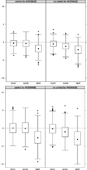
Figure 3 displays the differences between estimates using the imputed values and the true values for missing establishments for each of the three scenarios. Neither model was biased for the MAR1 scenario. Including $\mathsf{AVEWAGE}$ in the model minimized bias in the MAR2 scenario, as would be expected given that this was a key predictor of missingness. Both models yielded bias in the NINR scenario, however, there was modest improvement using the model which controlled for $\mathsf{AVEWAGE}$. These results highlight the importance of broadening the set of variables included in the imputation model as a way to make the missing at random assumption more tenable [Collins, Schafer and Kam (2001)].

Figure 3: Boxplot of the 250 differences between estimates using imputed values and those using the true values from the simulation study (using computer information system managers as the occupation). The estimates are for the nonresponding units only. The top figure displays the differences between mean occupational wage estimates and the bottom figure shows the differences between the 75th percentile estimates. Results are shown for the three different missing-data mechanisms used: MAR1, MAR2 and NINR. MAR1 depends only on employment size and being in large MSA, MAR2 is the same as MAR1 plus association with $\mathsf{AVEWAGE}$, while NINR depends only on the unobserved mean occupational wage.

5 Discussion

We proposed a flexible, yet explicit model for imputing missing occupational wages into categories. The model incorporates administrative wage data at the establishment level as well as geography, industry and other establishment characteristics to account for nonresponse bias. Unlike a weight-based method of adjustment for nonresponse, this imputation approach is able to extrapolate missing occupational wage values using establishment wages.

During the evaluation of this method, it was shown that the model generated imputations that more closely paralleled the observed relationship between the average wage and the observed occupational wage at that establishment compared to the existing OES method. At high levels of aggregation, where the response rates for OES are high (roughly 78%), the mean and quantile estimates of occupational wages were similar to those using the existing imputation method. However, more substantial differences were seen in estimates for sub-domains defined by industry and MSA.

The importance of broadening the set of variables to include $\mathsf{AVEWAGE}$ in the imputation model was also highlighted by the results of the simulation. Under the NINR simulation scenario, where nonresponse only depended on the occupational wage, there was some bias reduction using the model which controlled for $\mathsf{AVEWAGE}$. This occurred even though the simulations were based on the observed data from responding establishments, which tend to have lower $\mathsf{AVEWAGE}$ values than nonresponding units.

We chose a Cox proportional hazards model for our imputation process. This has a number of attractive features, including a flexible model for the baseline hazard (which is fit separately for each occupation as well as important industry classes) and the ability to cluster employees within establishment. Other models (such as a proportional odds model or a multinomial logistic model) might be considered as an alternative approach, though such approaches would have to be extended to allow stratification. In our own evaluation of these methods, none were better than one using a stratified Cox model. This may be a topic for future research.

The current OES procedures utilize a hot deck imputation for employment followed by a weighting method to impute missing wages. Our goal was to improve the estimation of occupational wage estimates utilizing auxiliary information by replacing their second-stage weighting procedure with an approach that accounts for differences in average wage at the establishment level. There are several options to account for errors due to the imputation. One approach would be to re-sample imputations within each jackknife replication pool, while adjusting the hot deck procedure so that the total number of employees for each unit are sampled from an appropriate (posterior) distribution. Further discussion and consideration of other options is a topic for future research.

These evaluations indicate that the new method is likely to produce imputed values that more closely match the missing values. This may lead to more accurate estimates of occupational wages produced by the OES.

Appendix: Details on incorporating establishment variables

When applying a method to a large survey like the OES one usually encounters a number of issues concerning the data that must be handled before a method can be put into practice. In this section we report on issues encountered while trying to incorporate the information from a few of the establishment-level variables in the model and discuss how they were handled.

.1 Classifying NAICS code

Because pay rates for certain occupations depend on the industry $(\mathsf{IND})$, it is an important factor to include in the model. However, there are over 1100 different NAICS codes and some occupations only exist in a small subset of the codes. Additionally, observed employment is very dense in some industry codes and sparse in others, and this pattern is occupation specific. Therefore, including each possible $\mathsf{IND}$ as a factor in the model is impractical.

We address this separately for each occupation code by clustering similar NAICS codes in order to form classes of industry codes that have relatively homogeneous pay structures for that occupation. The clustering is done using a nonparametric procedure (regression tree), recursively splitting on $\mathsf{IND}$, as a continuous variable. This yields classes where industry codes are close to similar industries and maintains the inherent hierarchical structure of NAICS codes. For example, all establishments with a six-digit code starting with 52 (52XXXX) are in the super sector “Finance and Insurance,” while all establishments with a code in the form 524XXX are in the subcategory “Insurance Carriers and Related Activities.” The code 5241XX defines the even more refined subcategory of “Insurance Carriers,” while 52413X refines this to “Reinsurance Carriers.” Also, this method automatically splits industries where that occupation is dense while aggregating industries where the occupation is sparse.

In order to produce homogeneous classes, the mean of the observed wage distribution is used as the dependent variable in the tree regression. The number of groups depends on the variability of the mean wages as well as the sample size, $n$, within each occupation. We specified a minimum size for each industry class of 80 observed establishments employing people with that occupation code. These classes are then used as stratification variables for the baseline hazard function.

For lawyers, with 4081 establishments in the survey (of which 2813 were observed), this resulted in a partitioning of NAICS nodes consisting of nine distinct nodes ranging from a minimum size of 192 (Node 13) to the largest node (Node 14) with a size of 1480. The partitioning also has the intuitively appealing classification of industries shown in Figure 4.

Figure 4: Results from regression tree partition of NAICS code for lawyers using observed mean wage. Each end node represents establishments employing lawyers in industries within a given range of NAICS codes. The boxplot shown at the bottom of each of the nine end nodes displays the distribution of the average wage rate for lawyers among these establishments. The nodes above the end nodes show where the recursive partitioning algorithm chose to split the industries. Most of the splits occur on the 6-digit industry codes between 51XXXX and 56XXXX, representing industries which often employ lawyers and among those where wage rates differ substantially.

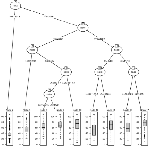
Most of the splitting occurred among the six-digit NAICS codes ranging from 51XXXX and 56XXXX which make up the information, financial and professional service industries. This is expected since these are the industries in which most lawyers are employed and for which the salaries have the most variability. Of the nine nodes all but three are composed primarily of industries in this range. One notable exception is local government (NAICS 999300), which also contains a large number of establishments with lawyers, dominated Node 2 (the node with the lowest average occupational wage).

For comparison, there were 21,089 establishments in the survey reporting employees with the occupational category customer service representative, of which 14,232 were observed. This yielded 16 distinct NAICS classes that were also interpretable and homogeneous with respect to average wage.

.2 Including MSA information

Similarly, occupational pay rates often depend on the location of the establishment, therefore, metropolitan statistical area ($\mathsf{MSA}$) is an important variable to include in the model. But as with industry, there are too many MSAs to include each MSA as a strata. Much of the association between occupational wage rates and the MSA in which the establishment is located is determined by the size of the MSA. Therefore, for most MSAs we include an indicator in the model for whether the establishment was in the largest of six size categories, but for areas with sufficiently large MSA’s (at least 250 establishments employing that occupation) the unique MSA label was also included in the model as a factor.

.3 Addressing irregularities in extreme QCEW values

The proposed method extrapolates occupational wage data at an establishment using$\mathsf{AVEWAGE}$ obtained from the administrative QCEW data. Observed OES and QCEW data suggest a positive association between an establishment’s computed occupational wage and $\mathsf{AVEWAGE}$ for every occupation considered during the empirical investigation. However, extreme values of $\mathsf{AVEWAGE}$ occur in the QCEW because of unusually high reported wage or low reported employment values (resulting in an unusually large $\mathsf{AVEWAGE}$) or low reported wage values (resulting in an unusually small $\mathsf{AVEWAGE}$).

Extremely high reported values for wages occurring in the QCEW are usually driven by very high bonuses paid during the quarter or large payouts taken by the owners of the establishment. Unusually low employment counts (even zero), when positive wages are reported, occur because employment data count only workers on the payroll during the pay period that includes the 12th day of the month, while all wages paid are reported as wages. Both of these lead to large $\mathsf{AVEWAGE}$ due to situations that are unlikely to be associated with the wage rates paid by the establishment.

Small reported earnings relative to the number of workers usually results from a small average number of hours worked by the employees at an establishment. Since the QCEW does not record number of hours worked, an establishment that has slowed down production for a period may have a large number of employees on the payroll who have worked minimal hours. This situation would lead to a small reported $\mathsf{AVEWAGE}$ for that establishment, but would likely be unrelated to the wage rates paid by the establishment.

Despite the strong evidence of an association between an establishment’s computed occupational wage and $\mathsf{AVEWAGE}$, this association is unlikely to hold at the extreme tails of $\mathsf{AVEWAGE}$. To address outliers in the values of $\mathsf{AVEWAGE}$, we recoded all values outside the middle 98% of the distribution. Values between the minimum and the 1.0th percentile were recoded to be the value of 1.0th percentile while values between the 99.0th percentile and the maximum were recoded to the 99.0th percentile value. This has the effect of changing relatively few of the reported values, but still protects us from over extrapolation.

References

- Abayomi, Gelman and Levy (2008) {barticle}[mr] \bauthor\bsnmAbayomi, \bfnmKobi\binitsK., \bauthor\bsnmGelman, \bfnmAndrew\binitsA. and \bauthor\bsnmLevy, \bfnmMarc\binitsM. (\byear2008). \btitleDiagnostics for multivariate imputations. \bjournalJ. R. Stat. Soc. Ser. C. Appl. Stat. \bvolume57 \bpages273–291. \biddoi=10.1111/j.1467-9876.2007.00613.x, issn=0035-9254, mr=2440009 \bptokimsref\endbibitem
- Bureau of Labor Statistics (2011) {bmisc}[auto:STB—2014/02/12—12:18:25] \borganizationBureau of Labor Statistics (\byear2011). \bhowpublishedOccupational establishment survey state operations manual (Appendix M: OES estimation procedures). \bptokimsref\endbibitem
- Chang and Kott (2008) {barticle}[mr] \bauthor\bsnmChang, \bfnmTed\binitsT. and \bauthor\bsnmKott, \bfnmPhillip S.\binitsP. S. (\byear2008). \btitleUsing calibration weighting to adjust for nonresponse under a plausible model. \bjournalBiometrika \bvolume95 \bpages555–571. \biddoi=10.1093/biomet/asn022, issn=0006-3444, mr=2443175 \bptokimsref\endbibitem
- Chen and Shao (2000) {barticle}[auto:STB—2014/02/12—12:18:25] \bauthor\bsnmChen, \bfnmJ.\binitsJ. and \bauthor\bsnmShao, \bfnmJ.\binitsJ. (\byear2000). \btitleNearest neighbor imputation for survey data. \bjournalJournal of Official Statistics \bvolume16 \bpages113–131. \bptokimsref\endbibitem
- Collins, Schafer and Kam (2001) {barticle}[pbm] \bauthor\bsnmCollins, \bfnmL. M.\binitsL. M., \bauthor\bsnmSchafer, \bfnmJ. L.\binitsJ. L. and \bauthor\bsnmKam, \bfnmC. M.\binitsC. M. (\byear2001). \btitleA comparison of inclusive and restrictive strategies in modern missing data procedures. \bjournalPsychol. Methods \bvolume6 \bpages330–351. \bidissn=1082-989X, pmid=11778676 \bptokimsref\endbibitem
- Cox (1972) {barticle}[mr] \bauthor\bsnmCox, \bfnmD. R.\binitsD. R. (\byear1972). \btitleRegression models and life-tables. \bjournalJ. R. Stat. Soc. Ser. B Stat. Methodol. \bvolume34 \bpages187–220. \bidissn=0035-9246, mr=0341758 \bptnotecheck related \bptokimsref\endbibitem
- Efron (1977) {barticle}[mr] \bauthor\bsnmEfron, \bfnmBradley\binitsB. (\byear1977). \btitleThe efficiency of Cox’s likelihood function for censored data. \bjournalJ. Amer. Statist. Assoc. \bvolume72 \bpages557–565. \bidissn=0162-1459, mr=0451514 \bptokimsref\endbibitem
- Groshen (1991) {barticle}[auto:STB—2014/02/12—12:18:25] \bauthor\bsnmGroshen, \bfnmE.\binitsE. (\byear1991). \btitleSources of intra-industry wage dispersion: How much do employers matter? \bjournalThe Quarterly Journal of Economics \bvolume106 \bpages869–884. \bptokimsref\endbibitem
- Holt and Smith (1979) {barticle}[auto:STB—2014/02/12—12:18:25] \bauthor\bsnmHolt, \bfnmD.\binitsD. and \bauthor\bsnmSmith, \bfnmT. M. F.\binitsT. M. F. (\byear1979). \btitlePost-stratification. \bjournalJournal of the Royal Statistical Society, Series A: General \bvolume142 \bpages33–46. \bptokimsref\endbibitem
- Kim and Kim (2007) {barticle}[mr] \bauthor\bsnmKim, \bfnmJae Kwang\binitsJ. K. and \bauthor\bsnmKim, \bfnmJay J.\binitsJ. J. (\byear2007). \btitleNonresponse weighting adjustment using estimated response probability. \bjournalCanad. J. Statist. \bvolume35 \bpages501–514. \biddoi=10.1002/cjs.5550350403, issn=0319-5724, mr=2381396 \bptokimsref\endbibitem
- Kott (2006) {barticle}[auto:STB—2014/02/12—12:18:25] \bauthor\bsnmKott, \bfnmP.\binitsP. (\byear2006). \btitleUsing calibration weighting to adjust for nonresponse and coverage errors. \bjournalSurvey Methodology \bvolume32 \bpages133–142. \bptokimsref\endbibitem
- Kott and Chang (2010) {barticle}[mr] \bauthor\bsnmKott, \bfnmPhillip S.\binitsP. S. and \bauthor\bsnmChang, \bfnmTed\binitsT. (\byear2010). \btitleUsing calibration weighting to adjust for nonignorable unit nonresponse. \bjournalJ. Amer. Statist. Assoc. \bvolume105 \bpages1265–1275. \biddoi=10.1198/jasa.2010.tm09016, issn=0162-1459, mr=2752620 \bptokimsref\endbibitem
- Lane, Salmon and Spletzer (2007) {bmisc}[auto:STB—2014/02/12—12:18:25] \bauthor\bsnmLane, \bfnmJ.\binitsJ., \bauthor\bsnmSalmon, \bfnmL.\binitsL. and \bauthor\bsnmSpletzer, \bfnmJ.\binitsJ. (\byear2007). \bhowpublishedEstablishment wage differentials. Monthly Labor Review 4 3–17. \bptokimsref\endbibitem
- Little (1982) {barticle}[mr] \bauthor\bsnmLittle, \bfnmRoderick J. A.\binitsR. J. A. (\byear1982). \btitleModels for nonresponse in sample surveys. \bjournalJ. Amer. Statist. Assoc. \bvolume77 \bpages237–250. \bidissn=0162-1459, mr=0664675 \bptokimsref\endbibitem
- Little and Rubin (2002) {bbook}[mr] \bauthor\bsnmLittle, \bfnmRoderick J. A.\binitsR. J. A. and \bauthor\bsnmRubin, \bfnmDonald B.\binitsD. B. (\byear2002). \btitleStatistical Analysis with Missing Data, \bedition2nd ed. \bpublisherWiley, \blocationHoboken, NJ. \bidmr=1925014 \bptokimsref\endbibitem
- Little and Vartivarian (2005) {barticle}[auto:STB—2014/02/12—12:18:25] \bauthor\bsnmLittle, \bfnmR.\binitsR. and \bauthor\bsnmVartivarian, \bfnmS.\binitsS. (\byear2005). \btitleDoes weighting for nonresponse increase the variance of survey means? \bjournalSurvey Methodology \bvolume31 \bpages161–168. \bptokimsref\endbibitem
- Phipps and Toth (2012) {barticle}[mr] \bauthor\bsnmPhipps, \bfnmPolly\binitsP. and \bauthor\bsnmToth, \bfnmDaniell\binitsD. (\byear2012). \btitleAnalyzing establishment nonresponse using an interpretable regression tree model with linked administrative data. \bjournalAnn. Appl. Stat. \bvolume6 \bpages772–794. \biddoi=10.1214/11-AOAS521, issn=1932-6157, mr=2976491 \bptokimsref\endbibitem
- Piccone and Hesley (2010) {bmisc}[auto:STB—2014/02/12—12:18:25] \bauthor\bsnmPiccone, \bfnmD.\binitsD. and \bauthor\bsnmHesley, \bfnmT. E.\binitsT. E. (\byear2010). \bhowpublishedUsing point and intervalized data in occupational employment statistics survey estimates. Bureau of Labor Statistics Survey Papers. Available at http://www.bls.gov/osmr/pdf/st100320.pdf. \bptokimsref\endbibitem
- Rubin (1976) {barticle}[mr] \bauthor\bsnmRubin, \bfnmDonald B.\binitsD. B. (\byear1976). \btitleInference and missing data. \bjournalBiometrika \bvolume63 \bpages581–592. \bidissn=0006-3444, mr=0455196 \bptnotecheck related \bptokimsref\endbibitem
- Schenker et al. (2011) {barticle}[mr] \bauthor\bsnmSchenker, \bfnmNathaniel\binitsN., \bauthor\bsnmBorrud, \bfnmLori G.\binitsL. G., \bauthor\bsnmBurt, \bfnmVicki L.\binitsV. L., \bauthor\bsnmCurtin, \bfnmLester R.\binitsL. R., \bauthor\bsnmFlegal, \bfnmKatherine M.\binitsK. M., \bauthor\bsnmHughes, \bfnmJeffery\binitsJ., \bauthor\bsnmJohnson, \bfnmClifford L.\binitsC. L., \bauthor\bsnmLooker, \bfnmAnne C.\binitsA. C. and \bauthor\bsnmMirel, \bfnmLisa\binitsL. (\byear2011). \btitleMultiple imputation of missing dual-energy X-ray absorptiometry data in the National Health and Nutrition Examination Survey. \bjournalStat. Med. \bvolume30 \bpages260–276. \biddoi=10.1002/sim.4080, issn=0277-6715, mr=2758877 \bptokimsref\endbibitem
- Therneau (2013) {bmisc}[auto:STB—2014/02/12—12:18:25] \bauthor\bsnmTherneau, \bfnmT.\binitsT. (\byear2013). \bhowpublishedA package for survival analysis in S. R package version 2.37-4. Available at http://CRAN.R-project.org/package=survival. \bptokimsref\endbibitem