AGN and quasar science with aperture masking interferometry
on the James Webb Space Telescope

Abstract

Due to feedback from accretion onto supermassive black holes (SMBHs), Active Galactic Nuclei (AGNs) are believed to play a key role in $\Lambda$CDM cosmology and galaxy formation. However, AGNs’ extreme luminosities and the small angular size of their accretion flows create a challenging imaging problem. We show James Webb Space Telescope’s Near Infrared Imager and Slitless Spectrograph (JWST-NIRISS) Aperture Masking Interferometry (AMI) mode will enable true imaging (i.e., without any requirement of prior assumptions on source geometry) at $\sim$ $65$ mas angular resolution at the centers of AGNs. This is advantageous for studying complex extended accretion flows around SMBHs, and in other areas of angular-resolution-limited astrophysics. By simulating data sequences incorporating expected sources of noise, we demonstrate that JWST-NIRISS AMI mode can map extended structure at a pixel-to-pixel contrast of $\sim$ $10^{-2}$ around an L=$7.5$ point source, using short exposure times (minutes). Such images will test models of AGN feedback, fuelling and structure (complementary with ALMA observations), and are not currently supported by any ground-based IR interferometer or telescope. Binary point source contrast with NIRISS is $\sim$ $10^{-4}$ (for observing binary nuclei in merging galaxies), significantly better than current ground-based optical or IR interferometry. JWST-NIRISS’ seven-hole non-redundant mask has a throughput of 15%, and utilizes NIRISS’ F277W (2.77µm), F380M (3.8µm), F430M (4.3µm), and F480M (4.8µm) filters. NIRISS’ square pixels are 65 mas per side, with a field of view $\sim$ $2\arcmin$ $\times$ $2\arcmin$. We also extrapolate our results to AGN science enabled by non-redundant masking on future 2.4 m and 16 m space telescopes working at long-UV to near-IR wavelengths.

1. Introduction

Supermassive black holes (SMBHs), with masses $\sim 10^{6}-10^{9}M_{\odot}$ are believed to lie in the centers of nearly all galaxies in the Universe (e.g. Kormendy & Richstone, 1995). When accreting, these SMBHs can outshine their host galaxy, with luminosities spanning $\sim 10^{10}-10^{16}L_{\odot}$ (e.g. Ho, 2008; Kauffmann & Heckman, 2009). The resulting active galactic nuclei (AGNs) and quasars are believed to play a key role in galaxy formation and, via feedback, in $\Lambda$CDM cosmology (e.g. Springel et al., 2006; Schawinski et al., 2007; Silk & Nusser, 2010). In spite of their importance, the combination of extreme luminosity ($\sim 10^{10}-10^{16}L_{\odot}$), small size ($\sim$pc) and large distance ($\geq 10$ Mpc typically) makes it very difficult to image details in most AGNs. Spectral and variability studies have allowed us to infer a great deal about AGNs. However high contrast and high resolution images would provide new, strong tests of models of AGN binarity, structure, fuelling and feedback, which in turn impacts models of galaxy formation and $\Lambda$CDM cosmology.

A non-redundant mask (NRM) placed in a pupil plane of a telescope converts a traditional single aperture telescope into an interferometer (e.g. Baldwin et al., 1986; Readhead et al., 1988; Tuthill et al., 1998; Monnier, 2003; Sivaramakrishnan et al., 2009a). This enables moderate contrast, high resolution imaging. This method has long been used with ground-based optical and near-IR telescopes to study faint structure and point sources around stars in our own Galaxy (e.g. Haniff et al., 1987; Tuthill et al., 2000; Monnier, 2003). However, ground-based optical and IR interferometers do not measure fringe phase reliably. Instead particular combinations of fringe phases known as closure phases are used to fit models selected a priori, because these closure phases are calibratable observables. Calibration of closure phases is accomplished by observing a known point source. In the cores of AGNs there are a wide range of expected structures, so true imaging provides more science than model fitting. However, due to atmospheric turbulence, ground-based model fitting of optical and IR interferometric closure quantities does not allow us to construct morphologies reliably (see e.g. Renard et al., 2011; Baron et al., 2012, and §2, §3.6, and §4, especially §4.1).

The James Webb Space Telescope (JWST) Near Infrared Imager and Slitless Spectrograph (Doyon et al., 2012) will deploy a non-redundant mask (NRM) in space (Sivaramakrishnan et al., 2012). Above the atmosphere fringe phase and amplitude should be easily measured in the optical and near-IR, enabling model-free imaging at a resolution of $\lambda/2D$ ($\lambda$ being the wavelength, and $D$ the telescope diameter or longest baseline length). Since space-based observing also provides both closure phases and closure amplitudes, those targets possessing known priors can utilize these closure quantities to improve estimates of model parameters. Good closure amplitudes improve model fits, especially those that include symmetric structures (e.g. Readhead et al., 1980). On the ground closure amplitudes have been of questionable utility in many cases, because changing atmospheric conditions make calibration very difficult. In this paper we demonstrate the potential of space-based NRM for AGN and quasar science. We focus on JWST-NIRISS’ Aperture Masking Interferometry mode (AMI), to show that it should, for the first time ever, be able to image details of the accretion flow in AGNs. We extrapolate our near-IR predictions to aperture masking on possible future optical/UV space telescopes to outline their potential for SMBH science.

In §2 we discuss how images of the extended accretion flow could help answer outstanding scientific questions concerning AGNs and quasars. In §3 using NIRISS in AMI mode as an example, we show how a space telescope can operate as an imaging interferometer, and make comparisons to ground-based instruments. In §4 we discuss what NIRISS in AMI mode could observe in some representative celestial objects. In §5 we briefly discuss NRM on possible future missions.

2. The need for imaging

AGN models are strongly constrained by spectral and variability studies, but not yet by imaging studies (apart from prominent jets). A (model fitted) dusty torus has been imaged in NGC 1068 due to uniquely favorable conditions–it is a very nearby Seyfert 2, and is therefore highly obscured by the torus, while still being bright enough to be seen using interferometric techniques, without requiring significant contrast (Raban et al., 2009). Images of AGNs at both moderate to high contrast and high resolution will show the morphology of structures feeding black hole accretion, and feedback on the host galaxy. Both are areas where geometry could rule out models. We outline several AGN science goals that require optical/infrared (O/IR) imaging, both those achievable with NIRISS in AMI mode and those that will require future instruments.

2.1. Dual and Binary AGNs

The standard cosmological model of hierarchical galactic mergers should produce large numbers of merging SMBHs. If both SMBHs are accreting, we should observe large numbers of dual AGN in galaxies. However, only a handful of dual AGN have been observed to date (e.g. Liu et al., 2010; Comerford et al., 2012). At optical wavelengths, dual AGN candidates are selected from nuclei displaying double-peaked narrow emission lines with velocity offsets relative to stellar absorption lines (e.g. Comerford et al., 2013). Follow-up in the near IR and optical can reveal tidal features and separated stellar populations (Liu et al., 2010). The projected spatial offsets between dual AGNs in SDSS selected samples are $\sim 1\arcsec$, corresponding to $\sim$kpc separations (Comerford et al., 2012). With an inner working angle (IWA) of $\sim 70$ mas, NIRISS in AMI mode will be capable of searching for dual AGNs in the near IR at angular separations at least an order of magnitude smaller than presently achieveable. A NIRISS AMI mode survey of low redshift galactic nuclei displaying double-peaked optical emission lines will find dual AGNs down to separations of $\leq 17$ pc and contrasts of $\leq 10$ mag in galaxies out to $\sim 50$ Mpc. Thus, NIRISS’ AMI will probe binaries closer to merger and with lower accretion rate (and lower mass) secondary SMBHs. In addition, space-based NRM (unlike ground-based NRM–see §3.6) will yield astrometric information on the galactic nucleus, allowing us to distinguish AGNs offset from the dynamical center of the galaxy. Astrometry in these cases allows us to test models of SMBH recoil and SMBH mergers where only the secondary is accreting.

2.2. How are AGNs and quasars fuelled?

For SMBHs to feed at the inferred fractions of the Eddington rate (Kauffmann & Heckman, 2009), large masses of gas must lose a large amount of angular momentum. At present we do not understand whether the process of angular momentum loss is continuous or a sudden, single, violent event. Nuclear bars, nuclear spirals or rings of star formation might provide a continuous supply of low angular momentum gas over a long time (e.g. Hopkins & Quataert, 2010; Schartmann et al., 2010). Or, fuel could be delivered by one-time events such as the infall of giant molecular clouds (Hopkins & Hernquist, 2006) or cloud bombardment from the halo (McKernan et al., 2010b). The maximum energy extractable from the mass reservoirs that fuel activity is $\sim\eta Mc^{2}\sim 4\times 10^{59}(10^{61})$ ergs respectively, where $\eta$ is the accretion efficiency ($\eta\sim 0.06(0.42)$ for a static (maximally spinning) black hole. Assuming $\eta\sim 0.1$ if a quasar is generated by accretion at the Eddington rate onto a $10^{8}M_{\odot}$ SMBH, then a quasar lifetime of 1(100) Myr requires a mass reservoir of $M\sim 2\times 10^{6}(10^{8}M_{\odot})$ respectively. Therefore, powering a quasar for $\sim 1$ Myrs requires fuelling by a mass equivalent to a giant molecular cloud. But the mass equivalent of an entire dwarf galaxy (probably in a minor merger) would be required to fuel the quasar for $100$ Myr. Evidently, if we can image fuelling structures around quasars we can constrain: the size of the mass reservoir, the lifetime and fuelling mechanisms. Many of these targets will be challenging for JWST. However, for 3C 273 (a $10^{9}M_{\odot}$ SMBH) to accrete at the Eddington rate ($\sim 20M_{\odot}$/yr) for only 10 Myrs, requires $\sim 2\times 10^{8}M_{\odot}$ of fuel. Such a reservoir should be visible in moderate to high contrast images of the regions around quasars $\sim 100$’s pc from the core (potentially observable by NIRISS in AMI mode). Beyond simple detection, images revealing the geometry of a fuelling structure will allow us to distinguish between models of continuous nuclear fuelling by a nuclear bar or spiral on one hand, and intermittent supply mechanisms on the other. Additionally, if no large reservoir is found we must consider models of quasar luminosity due to processes solely internal to the AGN accretion disk, for instance the migration of stars or compact objects within the quasar (Goodman & Rafikov, 2001; McKernan et al., 2011).

2.3. Constraining $\Lambda$CDM cosmology and theories of galaxy formation

Fuelling also directly impacts feedback–a key ingredient in $\Lambda$CDM cosmology–since the energy available for feedback is limited by the energy available through fuelling, and feedback can only occur while the AGN is active. The effects of feedback are also affected by geometry; hence imaging is an important tool for investigating feedback. We infer large mass outflows in many AGNs (McKernan et al., 2007; Miniutti et al., 2010). Such outflows can have a large impact on the host galaxy, suppressing star formation at late cosmological times (Springel et al., 2006; Sijacki et al., 2007; Silk & Nusser, 2010). Such suppression may be required to create galaxies as we see them today, possibly including the observed $M-\sigma$ relation between SMBH mass and stellar velocity dispersion in galactic bulges (Ferrarese & Merritt, 2000). The standard model of $\Lambda$CDM cosmology predicts hierarchical growth of structures, but may require significant AGN feedback in order to explain present-day structure in our Universe (e.g. Springel et al., 2005; Bower et al., 2006; Schawinski et al., 2007; McCarthy et al., 2010).

The impact of feedback from a quasar on its host galaxy depends on the total energy output, but also its duration and geometry. Constraining quasar lifetimes (as in §2.2) itself constrains feedback. If quasars are short-lived (Martini et al., 2003) we must re-think the role of AGN feedback in both galaxy formation and $\Lambda$CDM cosmology. Images will also allow us to determine the geometry of feedback. Broad versus collimated outflows, for example, can have very different effects on a host galaxy.

Nearby Seyfert galaxies are thought to be qualitatively similar to more distant quasars; fuelling, lifetimes and feedback remain key questions for these targets as well. If they are scaled down versions of quasars, high angular resolution, moderate contrast images of the structure of their fuelling regions (at few-10’s pc, well within the capability of NIRISS in AMI mode) can provide us with better models for their distant, brighter analogs.

2.4. Is the outer accretion disk stable?

Around SMBHs accretion disks should be unstable to gravitational collapse beyond $\sim 10^{3}$ gravitational radii ($r_{g}=2GM/c^{2}$). The instability criterion for gas disks is written in terms of Toomre’s Q parameter where

$$Q=\frac{\kappa c_{\rm s}}{\pi G\Sigma}$$ (1)

where $\kappa$ is the gas epicyclic frequency, $c_{\rm s}$ the gas sound speed and $\Sigma$ the disk surface density. A gas disk is unstable when $Q<1$. Since $\kappa c_{\rm s}$ drops more rapidly than $\Sigma$ in the outskirts of realistic gas disk models (e.g. Sirko & Goodman, 2003), we expect outer AGN disks to be vulnerable to clumping and rapid collapse into star forming regions (e.g. Shlosman & Begelman, 1987; Goodman & Tan, 2004). The AGN outer disk may therefore consist of many unstable, colliding clouds or density fluctuations (e.g. Nenkova et al., 2008; Mor et al., 2009). By imaging the outskirts of AGNs we can put limits on the number, size, extent, supply and luminosity of warm clouds in the outer AGN disk, directly testing the link between star formation and AGNs. NIRISS in AMI mode should image the outer accretion disk (torus) of about $20$ nearby AGNs; future missions will be required to assemble a larger ($\sim 100$’s) sample.

2.5. Searching for gaps and cavities in disks

Analogous to protoplanetary accretion disks, gaps and cavities can appear in AGN disks because of the presence of intermediate mass or SMBHs in the AGN disk (Artymowicz et al., 1993; Syer & Clarke, 1995; Ivanov et al., 1999; Levin, 2007; Kocsis et al., 2012; McKernan et al., 2014). The critical mass ratio ($q=q_{\rm crit}$) of secondary black hole to primary SMBH, above which a gap is opened in a disk is (Lin & Papaloizou, 1986; McKernan et al., 2014)

$$q_{\rm crit}\approx\left(\frac{27\pi}{8}\right)^{1/2}\left(\frac{H}{r}\right)^{5/2}\alpha^{1/2}$$ (2)

where $H/r$ is the disk thickness and $\alpha$ is the viscosity parameter (Shakura & Sunyaev, 1973). Images of gaps and cavities in AGN disks will directly constrain models of disk thickness and viscosity as well as models of intermediate mass black hole formation (McKernan et al., 2012). Imaging gaps or cavities in AGN disks requires much higher angular resolution than required for the tests outlined above, but may be possible with future telescopes.

2.6. Testing the standard model of AGNs

The standard model of AGNs assumes that orientation is a key determinant of observed properties (Antonucci, 1993; Urry & Padovani, 1995). However, random accretion events onto SMBHs should result in misalignment between axisymmetric galactic disks, AGN accretion disks and the spin of the SMBH (Volonteri et al., 2007). A rotating black hole will torque the accretion disk into its equatorial plane, leading to a warp in a misaligned accretion disk (Bardeen & Petterson, 1975; King & Pringle, 2006). Thus, obscuration in many AGNs could actually be due to misaligned or warped disks (Lawrence & Elvis, 2010). Images of the outskirts of AGN disks will reveal warps and misalignments between the disk and the plane of the host galaxy and test models of stochastic accretion. Alignment checks between host galaxy and fuelling region are achievable with NIRISS in AMI mode for tens of nearby AGNs; warping in the outer accretion disk is also observable for a smaller sample. Observing warps in the inner disk awaits instruments with smaller inner working angles.

Another important source of AGN obscuration is a large covering of orbiting clouds, independent of the AGN disk orientation (e.g. Krolik, 1999; Weedman & Houck, 2009; McKernan et al., 2010a). The orbiting clouds may originate among the unstable clumps believed to exist in the outskirts of the disk. Images of the outskirts of AGN disks (well within range of NIRISS in AMI mode) will constrain the geometry and ratio of orbital cloud mass to torus cloud mass and will allow us to test models of the origin of the orbiting clouds/stars (e.g. McKernan & Yaqoob, 1998; Risaliti et al., 2002; Turner & Miller, 2009, and references therein).

3. Imaging Extended Structures using JWST-NIRISS AMI

Here we describe the JWST-NIRISS AMI mode, our basic observational strategy and image reconstruction technique. To make our exposition accessible to those unfamiliar with imaging interferometry, we include 3 didactic appendices on basic topics. We begin with an explanation of the JWST-NIRISS AMI system; then discuss our simulated observations including sources of noise; we motivate and describe a move to the Fourier plane; we then explain our standard deconvolution strategy, showing results for several models. We then demonstrate some extensions to our standard method, and end with a comparison to ground-based capabilities. We highlight the importance of model-free image reconstruction with NIRISS in AMI mode, since a priori models of AGNs environs are extremely diverse.

3.1. JWST-NIRISS AMI implementation

NIRISS’s non-redundant mask consists of a seven-hole, $\sim 15$% throughput, titanium mask in a slot in the pupil wheel of NIRISS (Doyon et al., 2012). A full-scale prototype is shown in fig. 1. The NRM can be used with NIRISS’s F277W, F380M, F430M or F480M filters, which are centered at $2.77,3.80,4.30$ and $4.80\micron$, with bandwidths of 25, 5, 5 and 8%, respectively. Fig. 2 demonstrates the effect of increasingly complex apertures on PSF shape, ending with AMI mode’s theoretical PSF. Clearly, it is more complicated than the unmasked JWST PSF. However, the core of the NRM PSF is noticeably smaller, and it is surrounded by a deep null. The theoretical angular resolution is thus $0.5\lambda/D$ (65 mas at $4\micron$), which is more than a factor of 2 smaller than the $1.22\lambda/D$ Rayleigh limit. NIRISS’s 65 mas detector pixels are Nyquist-spaced at a wavelength of $4~{}\micron$. Fig. 3 shows both oversampled and detector pixel-sampled PSFs (all simulated sources of noise are included in the last panel). The NRM image is most useful in a region between an inner and outer working angle (IWA and OWA). For NIRISS, the IWA is $0.5\lambda/D$, where $\lambda$ is the wavelength and $D$ the primary mirror diameter or longest baseline. The OWA is 4–5 $\lambda/D$ — at wider angular scales direct imaging is more efficient than NRM. Thus NIRISS’ AMI mode is most interesting at separations between about 65 mas and 600 mas. Further work may show that in the shortest wavelength filter, F277W, AMI observations could be dithered to provide slightly smaller IWA than 65 mas (Koekemor & Lindsay, 2005; Greenbaum et al., 2013).

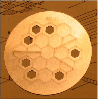
Figure 1.— A prototype of the NIRISS 7-hole non-redundant pupil mask (AMI mode) with engraved outline of primary mirror segments and secondary supports. Engraving is on the reverse side of the mask, so this image is looking through the back of it (flip and rotate to compare to figure 2). The mask has undersized holes compared to the segment size to mitigate against pupil shear up to 3.8$\%$. The projection of the JWST pupil is nominally circumscribed by a circle 39 mm in diameter. The part diameter is 50 mm.

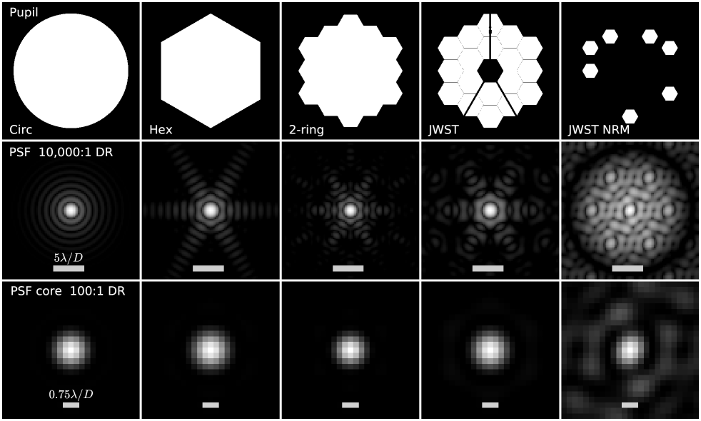
Figure 2.— A comparison of the point spread functions of different shaped apertures. The top row shows apertures as labelled. The middle row shows the corresponding PSFs with 10,000:1 dynamic range, at consistent stretch and pixel scale. The bottom row shows the cores of the same PSFs with 100:1 dynamic range. Note the relatively small core, and deep null, surrounding the JWST NRM PSF.

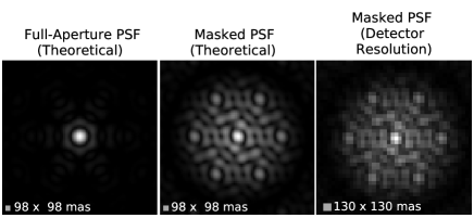
Figure 3.— The simulated point spread function for JWST NIRISS, displayed at the same dynamic range. Panels a, b, c from left to right: a) Oversampled by 2x, no noise, generated from a simulated observation of a 7.5 mag point source at 4.5$\micron$. b) As for a), but with the addition of NRM. c) Similar to b), but sampled at the resolution of the NIRISS detector (65 mas per pixel–undersampled given our theoretical resolution). Panel c) also includes realistic flat-field noise, photon noise read noise, intra-pixel sensitivity variations and telescope pointing error, for a 0.66 (0.42) sec integration in F380M, F430M (F480M) filters. Pointing error is (just) detectable by eye. See text for details of noise model and extrapolation to various filters.

3.2. Simulated observations and noise sources

We simulated observations of a 7.5 magnitude (mag) point source with NIRISS in AMI mode, conservatively assuming a detector with a $1\%$ bandpass centered on 4.5$\micron$. Exposure times to actual NIRISS filters centered on $3.80,4.30,$ and $4.80\micron$ are extrapolated from our initial simulations; what we simulated as a 1 second exposure would actually take 0.25 seconds with NIRISS F380M or F430M and 0.16 seconds using NIRISS F480M, given their 5, 5 and 8 % bandwidths, respectively. The observation consisted of 10 sequences of $N_{exp}=28$ exposures, each exposure equivalent to 0.66 (0.42) seconds for the F380M, F430M and (F480M) filters, respectively. Simulated noise sources included: a polychromatic PSF according to a specified transmission profile; pixel flat-field error of $0.1\%$; variable intra-pixel response with a Gaussian profile (1 at center, $0.8\pm 0.05$(rms) at the corner); read noise; dark current; background and photon noise; a pointing error of 5 mas rms per axis assumed between each exposure. We expect spectral smearing ($\sim\lambda/\Delta\lambda$) to be negligible when working within $2.5\lambda/D$.

Observations were simulated on a grid 11x finer than NIRISS pixels. To simulate a PSF calibrator observation, the noisy point source exposures were binned up by a factor of 11, as shown in the last panel of Fig. 3. We generated a model of extended structure around the point source AGN on the same oversampled grid; convolved the model image with a noiseless oversampled PSF. We then shifted the oversampled, convolved model image to match the pointing error of the $N_{exp}$th exposure of the simulated noisy point source sequence. We then binned up the noiseless, shifted, convolved extended structure by a factor of 11 and added it to the noisy point source observation sequence (with matching pointing error). Our approach is simpler than simulating the point source together with extended structure through the whole optical path including noise, since noise sources associated with the point source will dominate. Fig. 4 shows our fiducial extended structure model and the resulting NIRISS AMI mode interference fringes. Our model is a horizontal bar, 9 NIRISS pixels long (585 mas), with integrated flux of 8.5 mag, around a 7.5 mag point source AGN. We also considered models non-aligned with our detector grid, which showed similar behavior.

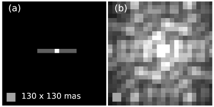
Figure 4.— Fiducial toy model of extended emission and simulated fringes. a) A model of extended emission around a point source, shown at NIRISS detector resolution. We have chosen a horizontal bar (one model for AGN fuelling), surrounding a 7.5 mag unresolved point source and ignore host galaxy background. The bar is 9 NIRISS pixels long (585 mas), with integrated flux of 8.5 mag. Note this image is shown for reference; when simulating observations, we convolve our toy model with the 11x oversampled PSF, before adding the noisy point source and rebinning fringes to the scale of the NIRISS detector (see Fig. 3). Thus, in simulated observations, the bar is 1/11th of a NIRISS detector pixel in width (but length as shown). b) Simulated NIRISS AMI mode observation of the bar described in a). Integration time is 0.66 (0.42) sec in F380M, F430M (F480M) filters, and noise sources are described in the text. Compare to point source in Fig. 3c. Source structure is not apparent by eye.

We used the first 28 noisy exposures of the point source as our PSF calibrator, so exposure times were 18.48 (11.76) sec at one orientation for the F380M, F430M and (F480M) filters. The remaining 9 sequences of 28 exposures (with added extended structure and different noise realizations) were used to simulate science target exposures, so science exposure times were 166.32 (105.84) sec at one orientation for the F380M, F430M and (F480M) filters.

3.3. Fourier plane operations

A simple clean (Högbom, 1974) deconvolution (using IDL’s clean.pro), is shown in the left panels of Fig. 5. Our pointing errors are large enough (at only 8% of a NIRISS pixel) to introduce significant artifacts in the reconstructed image. Instead we proceed by zero-padding the images and taking the FFT of all exposures (calibrator and science target). We decompose the results into amplitude ($A({\bf u})$, e.g. Fig. 6) and phase ($\phi({\bf u})$, e.g. Fig. 7) of the complex visibility (for those new to interferometry, see appendix A). A change in telescope pointing introduces a uniform phase shift in the interference fringes (see appendix B), while amplitudes are unaffected. In Fourier space this becomes a slope across the Fourier phase plane. Therefore if our exposures are short enough to be characterized by a single pointing, we can fit and subtract a plane from the raw Fourier phases ($\phi$) of each exposure; this yields sub-pixel aligned phases ($\phi^{\prime}$). For convenience, we co-add visibilities for the calibrator and science target exposures respectively, forming a single set of sub-pixel aligned visibilities for each observation.

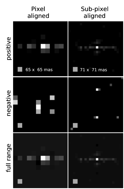
Figure 5.— Clean models for naive versus sub-pixel aligned deconvolution. All panels are displayed with a square root stretch. Left panels: A simple clean deconvolution of science target fringes (like those shown in Fig. 4b), using IDL’s clean.pro and point source calibrator fringes (like those shown in Fig. 3c) for the PSF. Images were aligned to pixel accuracy. Integration times are 2.8 (1.8) min on target and 18 (12) sec on the calibrator in F380M, F430M (F480M) filters. At NIRISS pixel scale the bar should be only 9 pixels long (including the point source). Note also the relatively large negative artifacts near the point source. Though pointing errors are small compared to a detector pixel, misalignments between the target and calibrator are significant enough to smear out the reconstruction. Shorter integrations result in less smearing but still produce large negative flux components and other artifacts comparable to or brighter than the extended structure shown here. Right panels: Clean model obtained using Fourier methods to align images to sub-pixel accuracy, as well as the addition of an observation at a second orientation (integration times are doubled from the first panel) and using MIRIAD clean. Pixels are $\sim$half the size of NIRISS, so the bar should be 18 pixels long (including the point source). Gain (0.1) and number of iterations (250) in the clean loop was the same for each panel. See text and Fig. 11 for further details on the right panels.

Figs. 6 and 7 show our maximum ${\bf u}$ plane (Fourier domain of our images) coverage at one orientation; note the gaps in coverage. Our ${\bf u}$ plane is equivalent to the radio interferometric $(u,v)$ plane. Fig. 8 shows the improved coverage for combined observations at two orientations, at $0^{\circ}$ and $90^{\circ}$, corresponding to JWST observations separated by a few months. We simulated observations at the second orientation by generating an identical extended source image rotated by the roll angle and proceeded as above. We then rotate the visibilities in the ${\bf u}$ plane by the roll angle. For the rotationally symmetric point source calibrator, we simply rotated the visibilities. Note that the roll angle (or, equivalently, the timing of the second visit) does not require fine-tuning. Of course, for future space missions, if two complementary masks were available in a pupil wheel, near-simultaneous, complete ${\bf u}$ plane coverage could be achieved.

Note the pattern of extended ‘splodges’ in the ${\bf u}$ plane, rather than points or tracks (as in radio interferometry). The total number of independent data points in Fourier space is equal to the number of pixels in image space (without windowing). Visibilities at splodge centers (e.g. Fig. 9a) provide the only fully independent (non-redundant) information, but away from the centers there is additional, partially independent information. This additional information is not usually extracted in ground based O/IR observations (see appendix B). By extracting the visibilities at points away from the splodge centers (i.e. away from those corresponding to the aperture center-to-center baselines) we get more imaging information in an observation than is possible from the ground. Target and calibrator visibilities are extracted at identical ${\bf u}$ coordinates, chosen by analyzing the calibrator data. Fig. 9c shows the ${\bf u}$ extraction pattern used to generate the bottom-right panel of Fig. 5. Appendix B discusses the effect of different extraction patterns on image reconstructions.

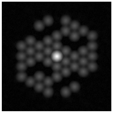
Figure 6.— Amplitude splodges from a simulated noisy JWST-NIRISS AMI mode observation of a 7.5 magnitude point source with a 0.66 (0.41) sec integration in F380M, F430M (F480M) filters, and noise sources as described in the text. These amplitudes come from the FFT of the image in Fig. 3c, zero-padded by a factor of 4.

Figure 7.— As Fig. 6, except for phase splodges. Note that in ground-based O/IR, fringe phases cannot be obtained, so closure phase and source priors must be used to obtain astrophysically interesting information.

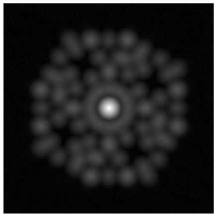
Figure 8.— Greatest ${\bf u}$ plane coverage possible given 2 observations separated by a roll angle of 90 degrees. Two sets of amplitude splodges (as for figure 6) with the second rotated by 90 degrees to the first. Extraction reduces the coverage further (see figure 9, last panel, for comparison, and appendix B).

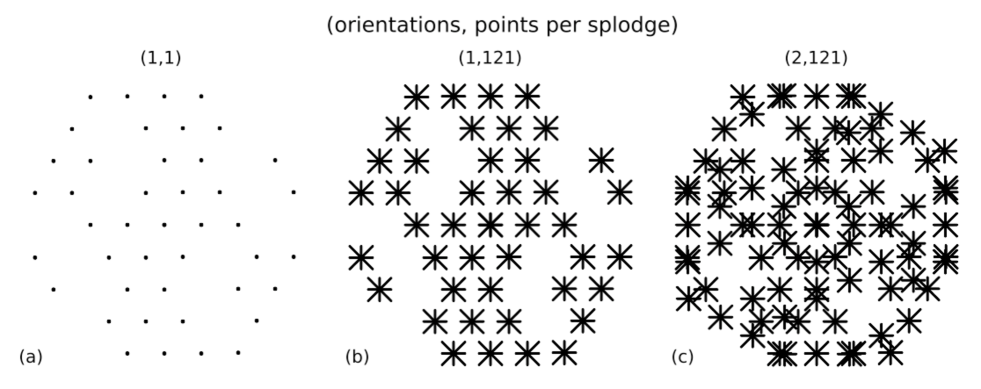
Figure 9.— Fourier (${\bf u}$) plane coverage after extraction. a) Extraction at one orientation, using only ${\bf u}$ splodge centers. b) Extraction at one orientation, but using 15x8 additional points per splodge, arranged as the vertices and bisectors of squares centered on the splodge; each square is two pixels larger than the previous one. c) Our standard extraction, as for panel b) but observing at 2 orientations. See appendix B for further details.

3.4. Deconvolution

We pass the sub-pixel aligned, extracted visibilities to MIRIAD (Sault et al., 1995), a radio interferometric software package. We concatenate visibilities from multiple orientations, and separately ‘invert’ (inverse Fourier transform) calibrator and target data, as shown in Fig. 10 (see appendix B for details). We have recovered our original fringes, now properly aligned for deconvolution, and weighted according to their ${\bf u}$ plane coverage (the weighting is non-uniform due to the combination of multiple orientations and the lower weighting of off-center extracted points). We have chosen an image plane pixel scale approximately twice as fine as our original detector images (35.6 mas). Pixel scale and signal-to-noise ratio (SNR) per pixel can be traded in any deconvolution scheme–this is one effect of various weighting schemes (see Briggs, 1995, and appendix B). While this trade also exists for full-aperture imaging, the inherently smaller PSF core and consequent improvement in theoretical angular resolution of an NRM system means that any result achievable with a full-aperture deconvolution can be improved upon in NRM imaging.

We use the normalized inverse Fourier transform of the extracted, sub-pixel aligned calibrator visibilities as our PSF (or ‘dirty beam’, $B$). This contrasts with the standard radio strategy of using the inverse Fourier transform of the target visibilities, with $(A,\phi)=(1,0)$ as the ‘dirty beam’ or PSF. Because we include ${\bf u}$ points away from splodge centers, our technique is equivalent to constructing a full Spatial Transfer Function. We use our PSF to clean the inverse Fourier transformed, extracted, sub-pixel aligned target visibilities (or ‘dirty map’, $I^{\prime}_{\rm fringe}$). We choose the smallest useful clean box. For the cases we show this was a square region 32 pixels on a side, centered on the brightest pixel in the fringe image. If we wish to image larger regions, we can do so up to a region one-quarter the size of the PSF; alternatively, we can use multiple pointings to construct a mosaic of extremely large fields.

We show the clean model and restored map in Fig. 11 (see appendix B for definitions). The clean model is the same as that shown in the bottom right panel of Fig. 5 and compares well with the input model shown in Fig. 4a. For NRM systems which capture fringes as gridded detector images (like NIRISS), the most useful interpretation of the data is obtained by viewing and comparing both the clean model and the restored map.

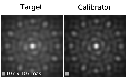
Figure 10.— Science target and calibrator fringes shown on square root stretch. a) Left panel shows inverse FT of sub-pixel aligned, extracted visibilities of observations at 2 orientations of our fiducial bar model. The target was observed for a total of 5.5 (3.5) min (half at each orientation) with NIRISS centered on $3.80,4.30,(4.80)\micron$ respectively. Pixel scale is twice as fine as the JWST-NIRISS detector pixel scale. b) Right panel shows the same but for the point source calibrator observations. Total exposure time is 37 (24) sec with NIRISS, centered on $3.80,4.30,(4.80)\micron$ respectively. This is our PSF. Note the structural similarities between the two panels, but the left panel shows significant ‘filling in’ of flux in the darker regions, due to the extended structure.

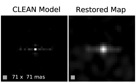
Figure 11.— Clean model and restored map from simulated observation of target shown in Fig. 4a. a) Left panel shows MIRIAD clean output of Fig. 10a, using Fig. 10b as the PSF. Note that when we inverse FT our visibilities, we chose a pixel scale twice as fine as the JWST NIRISS detector pixel scale, so while the input bar (in Fig. 4) is 9 pixels long, a perfectly recovered clean model should be 18 pixels long. Our reconstructed bar is 17 pixels long (including point source), and recovers $>90\%$ of the extended structure flux. b) Right panel shows the restored map from MIRIAD restor, using a symmetric Gaussian of FWHM=71 mas, for the restoring beam. See appendix B for further details of clean and restor.

Other models: Fig. 12 shows image reconstructions for some other extended emission models, including short and asymmetric bars and a ring (using the same techniques and exposure times as above). The second row demonstrates the recovery of a 9 NIRISS pixel long bar, at an integrated flux of 9.5 mag, or 2 mag integrated contrast, equivalent to 4.4 mag pixel-to-pixel contrast ($\sim 10^{-2}$), in 5.5 (3.5) min at $3.80,4.30,(4.80)\micron$. Assuming SNR improves as $\sqrt{t}$ (i.e. we are photon noise limited), we should reach 5 mag of contrast (pixel-to-pixel) imaging extended structures in less than 10 minutes.

All results presented thus far use clean, without the use of a model prior or selfcal (which would incorporate closure phase and closure amplitude information–see appendix C for definitions). Much of ground-based optical interferometry is used to measure a small number of parameters e.g. separation, contrast and position angle for two point sources. However, this approach will not work for sources with complicated extended structure, such as AGNs, where prior models are extremely diverse and have large numbers of variables. We note however that more advanced image reconstruction techniques are available (Baron et al., 2012, and references therein). We have not investigated their use on space-based data and offer our simulations as a conservative estimate of extended source imaging capabilities.

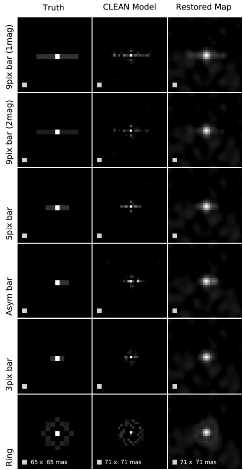
Figure 12.— Input model, clean model and restored map for a variety of sky geometries. All images displayed on a square root stretch. First column is input model at NIRISS resolution (65 mas per pixel), second column is resulting clean model and third column is the restored map, both with pixels half the size of NIRISS detector pixels. Features in the first column should be same linear size in columns 2 and 3. First row: same as Fig. 4a and 11. Second row: as for first row but the integrated flux from the bar is 9.5 mag (2 mag fainter than the point source). Third row: horizontal bar 5 NIRISS pixels long (325 mas), with the same surface brightness as the bar in the first row. Fourth row: similar to the third row, but with the left side of the bar missing. Fifth row: horizontal bar 3 NIRISS pixels long (195 mas), with the same surface brightness as the bar in the first row. Sixth row: circular ring of diameter 5 NIRISS pixels (325 mas). Ring has an integrated flux of 8.5 mag.

3.5. Other strategies

We have investigated some extensions to the simplest clean reductions, shown in Fig. 13. Selfcal enforces closure relations on visibility data when a model prior allows calculation of ‘expected’ closure phases (CPs) and closure amplitudes (CAs). It assumes all departures from expected relations are due to uncorrelated, aperture-specific errors, and computes a complex ‘gain’ for each aperture which corrects for those errors. For our science targets, we cannot guarantee the existence of such priors; however, our calibrator is known to be a point source, so applying selfcal to that data might be expected to improve our PSF measurement and the SNR in our image reconstructions. Unfortunately, CP and CA relations are not correctly defined by MIRIAD’s selfcal for $(u,v)$ points away from splodge centers (see appendix C for details). In addition, errors in our simulated data are not aperture specific, so unlike in the radio, it is not sensible to apply the ‘gains’ derived from our calibrator observations to our science observations (this may change in actual operations). Fig. 13 shows the clean model, restored map, residual map and ${\bf u}$ plane coverage for a series of experiments, all using our fiducial input model of a horizontal bar 585 mas long, with an integrated flux of 8.5 mag, surrounding a 7.5 mag point source. Selfcal experiments are indicated in red (CAL if used on the point source calibrator or TGT on the science target), while comparison results without selfcal are indicated in black. We also list the (absolute value of) residual flux as a percentage of the (absolute value of) flux in the input fringe image. We include a reduction using a simulated noiseless point source for a PSF–note the residuals decrease only slightly from our standard reduction.

As can be seen in Fig. 13, application of selfcal does not improve our image reconstructions, and in many ways makes them worse. Importantly, our source structure is plainly visible in many of the residual maps where selfcal was applied. In general, applying selfcal to our PSF improves our characterization of the PSF core (or main beam of our dirty beam). This reduces or eliminates the artifacts in our clean models appearing nearest the point source. However, selfcal significantly increases the noise level in the wings of the PSF (sidelobes), as seen in the increased level of artifacts distributed throughout the clean models and the increase in residual flux; the bar does not stand out as strongly in the restored maps. Although it is mathematically incorrect to do so, we did try to apply selfcal to splodge center and offset visibilities with no improvement. When applying selfcal to our science target, we must decide on a prior–we tried 1) a point source, 2) the output of our ‘blind’ standard reduction, and 3) an iterative approach. When modelling the science target as a point source, clean still recovers a bar feature, albeit with higher residuals than our standard reduction. In real operations, such an exercise might give additional confidence that features in a recovered image were not artifacts. The iterative sequence uses the output of our standard reduction (appropriately clipped) as our input model for selfcal. The following row uses the clean model from the row above (again clipped) as the input model for selfcal, and so on down the columns. While we might hope such an approach would allow us to improve our science image even in the absence of priors, Fig. 13 implies that this will not be possible for sources requiring significant dynamic range. Artifacts quickly appear at levels close to that of the extended structure (probably this results from the same core/wings noise shift seen in our calibrator experiments); the clip level required to exclude artifacts also excludes large portions of the real structure, making improvements over multiple iterations negligible.

We also simulated a noiseless observation of a point source, and used our standard (noisy) calibrator observations to clean them. The results are shown in Fig. 14; we note that the level of noise in the restored map is about $10^{-2}$ of the point source, and suspect that noise in our calibrator observations is presently limiting the contrast achievable via imaging. If JWST is sufficiently stable and well-characterized on-orbit, we may be able to acheive higher contrasts using a noiseless simulated PSF; even if calibrator observations are required (as is likely), longer calibrator integration times should improve achievable contrasts (also see the smaller residuals in the Fig. 13 panels where a noiseless point source was used for the PSF).

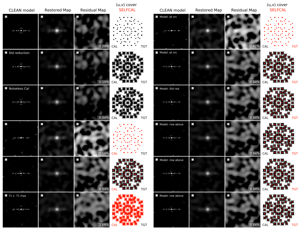
Figure 13.— Selfcal experiments, with non-selfcal comparisons. All experiments used our fiducial bar for a science target. Fourier plane coverage is identical between calibrator and science target observations for a given experiment; red points in the (u,v) cover column indicate selfcal was applied to those points for either the point source calibrator (red CAL) or the science target (red TGT). The percentage of flux remaining in residuals relative to the flux in the original fringe image is displayed in the bottom right corner of the residual map. All images are shown on a square root stretch; the residual maps are shown with the same range, so fainter features from frame to frame indicate smaller residuals. Many selfcal residuals show significant bar structure. Left columns, first 3 rows (no selfcal): Increasing ${\bf u}$ coverage improves our image reconstruction, reducing artifacts, residuals and more fully recovering the bar. Using a noiseless calibrator slightly improves residuals. Left columns, last 3 rows (selfcal on PSF): Using selfcal decreases the number and brightness of artifacts immediately adjacent to the point source in the clean models, but increases the number and brightness of scattered artifacts. Residuals are also higher. Right columns (selfcal on science target): Selfcal input model is indicated for each row at the top of the clean model (bottom 4 rows are an iterative sequence). Artifacts and residuals behave similarly to selfcal on PSF reductions.

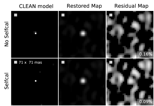
Figure 14.— Noiseless point source science target. We show the clean models, restored maps and residual maps for simulated observations of a noiseless point source, using our standard noisy point source observation as the PSF ((u,v) coverage is as for our standard reductions). We show results both with and without the use of selfcal. The level of residuals is comparable to that found in our standard reduction, and implies that our noise floor may be set by noise in our PSF. On orbit, this could be mitigated by longer calibrator observations and/or use of noiseless simulated PSFs. As in Fig. 13, use of selfcal increases the level of scattered artifacts in the clean models, but decreases them immediately surrounding the point source.

3.6. Comparison with Ground-based systems

Ground-based O/IR interferometers cannot measure absolute phase without resorting to exceedingly short (millisecond) exposures for atmospheric freezing (e.g. Haniff et al., 1987). Because of read-noise, this limits ground-based phase measurements to the very brightest objects. As Monnier & Allen (2013) state: ‘Without valid phase information accompanying the visibility amplitude measurements, one cannot carry out the inverse Fourier Transform that lies at the core of synthesis imaging and the clean algorithm specifically.’

The ‘images’ produced by ground-based O/IR interferometers depend on closure phase to partially recover otherwise inaccessible phase information. Instead of inverse Fourier Transforming the fully measured complex visibilities (as we do with AMI), ground-based O/IR imagers rely on modeling the amplitude and closure phase expected given a prior model of the source. Importantly, meaningful results depend on the accuracy of the model, where the number of free parameters is fewer than the number of equations available. An interferometer with $N$ apertures generates $N\choose 2$ independent phases, but only $N-1\choose 2$ independent closure phases (Readhead et al., 1988). As $N$ grows large, this discrepancy grows smaller, but for e.g. VLT’s NaCo SAM with $N=7$, closure phase only recovers 71% of the phase information. For AGNs, where environments are likely to be complicated, and not well modeled by simple a priori models with few parameters, this is a major barrier to advances from the ground.

Space holds other advantages, particularly for AGN science. Without phase, there can be no absolute astrometry, only relative astrometry. If we wish to compare e.g. the geometry of a torus or mass reservoir in the IR with the geometry of a jet from the radio (to look for differences in alignment), absolute astrometry is required (radio interferometers do get phase and absolute astrometry from the ground). Looking for offset AGNs also requires absolute astrometry.

The phase problem arises again if we wish to perform very wide-field mosaicking. Mosaic fields are limited to the size of the isoplanatic patch using ground-based optical interferometers (due to atmospheric instability and the guide star field-of-view limitations of AO systems (Fried, 1966)). At L-band this is slightly larger than half an arcminute (Monnier & Allen, 2013). Very wide-field mosaicking is more likely to be used for non-AGN science (though mapping of large scale jet interactions might call for such a technique), but we note the issue here for its importance to other subfields (e.g. ISM). The size of the patch also decreases at shorter wavelengths so mosaicking could be a critical advantage for space-based NRM observations at optical wavelengths in future missions.

There are also advantages to measuring amplitudes from space. Our amplitudes are measured with a higher signal-to-noise ratio than for similar ground-based systems, as expected given the greater stability of space-based systems and the lower thermal background. Specifically, we expect $\sim 10^{-14}$ thermal photons s^-1 pixel^-1 at F480M, based on an operating temperature of $50$ K and a circular mirror of radius $3.25$ m. Also, space-based systems can, uniquely in the O/IR, measure closure amplitude.

Though we do not use it in our imaging reductions, we do measure closure amplitude (CA), as well as closure phase (CP). These can be used to identify sources which depart significantly from point source geometry; CA is particularly effective for this purpose. We show in Fig. 15 the closure phase and closure amplitude, respectively, computed for our AMI observation of a point source (black), as well as for extended source bar models like that shown in Fig. 4 (1, 2, and 5 mag contrasts in red, green and blue, respectively–bars were observed for 2.8 (1.8) min at F380M, F430M (F480M)). We plot CP (CA) against the total length of the baselines contributing to each aperture triangle (quad) in arbitrary units. Though there are 35 triangles (quads) only 15 (14) are independent. The black points are the values for a noiseless point source (which depart from theoretical expectations due to pixellation); we computed CP and CA for 10 noisy realizations of our standard point source calibrator observations (18.48 (11.76) sec at F380M, F430M (F480M)) and found the standard deviation for each set of baselines. The plotted error bars are the usual standard deviation multiplied by 35/15 (35/14).

From the plot, we see that CP alone is barely able to distinguish the 1mag bar from a point source; by contrast, CA alone is able to distinguish a 5 mag fainter (integrated flux 12.5 mag) bar from a point source in less than 3 minutes. Performing a chi-squared test on the data, we find the 5 mag contrast bar data inconsistent with a point source at $5\sigma$ significance. This corresponds to a point-to-point contrast of $\sim 10^{-3}$, equivalent to the binary detection ability of VLT NaCo SAM (e.g. Lacour et al., 2011, and note that binary detection is an easier task than extended structure detection because of the limited number of degrees of freedom in the system and asymmetry, to which CP is more sensitive). The remarkable stability of CA is what allows us to acheive this contrast. Assuming the standard deviation increases with exposure time ($t$) only as $\sqrt{t}$ (i.e. if we are photon noise limited, which is likely to be true for the brightest targets) implies that a short $\sim$1.7 (1.1) ks NIRISS AMI exposure, could distinguish an extended bar at 7 magnitudes total flux contrast from a point source at $5\sigma$ statistical significance. This represents a point-to-point contrast of $\sim 10^{-4}$, or an order of magnitude better contrast than anything obtainable from ground-based O/IR interferometry. We caution that the chi-squared significance will be non-uniform depending on the science target structure and orientation.

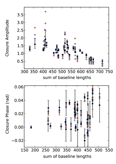
Figure 15.— Closure phase (in radians) and closure amplitude for a 7.5 mag point source (black) and noisy observations of 585 mas horizontal bars surrounding a 7.5 mag point source at 1, 2, and 5 mag integrated flux contrasts (red, green and blue, respectively). Total baseline length is in arbitrary units. Black circles represent CP (CA) values for a noiseless point source, which depart from theoretical expectations due to pixellation. Error bars are based on measured variance of CP (CA) for each baseline in 10 noisy point source observations, and show $1\sigma$ departures corrected for the number of independent CPs and CAs.

4. Example AGN targets

Table 1 lists targets for JWST-NIRISS AMI and future space-based NRM missions, spanning a range of activity types and black hole masses ($M_{\rm BH}$). Figure 16 shows the science topics within reach of the various missions. Since the size of an AGN central engine is supposed to scale with $M_{\rm BH}$ (Antonucci, 1993; Urry & Padovani, 1995; Peterson et al., 2004), NIRISS AMI will probe different structures around nearby AGNs with $M_{\rm BH}$ spanning $10^{6-9}M_{\odot}$. Column 8 in Table 1 lists the regions which can be imaged with JWST-NIRISS AMI, spanning (IWA,OWA)=(75,600) mas assuming $\lambda=4.8\mu$m. JWST-NIRISS AMI can image the outskirts of nearby AGNs as well as occasional flaring in otherwise quiescent nuclei (Sgr A*, M31). In nearby Seyferts, NIRISS AMI images will distinguish between models of continuous AGN fuelling (spiral or bar inflows from further out) and intermittent accretion events. Columns 9 & 10 in Table 1 list region sizes that could be imaged with future missions: a UV/optical-band Astrophysics Focused Telescope Assets (AFTA) with a 2.4 m primary mirror ($\lambda\sim 400$nm) and Advanced Technology Large-Aperture Space Telescope (ATLAST), a proposed optical mission ($\lambda\sim 500$nm) with a 16 m primary mirror. Possible future missions are discussed further in §5. Here we discuss detailed science goals for NIRISS AMI in several archetypal sources: NGC 4151, 3C 273 and M31.

Table 1Galactic nuclei targets for NRM on Space Telescopes

Name	RA	Dec.	$D_{L}$	log($M_{BH}$)	AGN	Apparent	JWST	AFTA	16m ATLAST
						Magnitude	4.8$\mu$m	400nm	500nm
	(J2000)	(J2000)	(Mpc)		class	(for aperture)	inner-outer	inner-outer	inner-outer
						(mag)($\arcsec$)	(pc)	(pc)	(pc)
(1)	(2)	(3)	(4)	(5)	(6)	(7)	(8)	(9)	(10)
NGC 4151	12 10 32.6	39 24 21	016.900	7.1	Sy 1	$6.6\pm 1$string(6)	6.2–49.9	1.41–11.3	0.3–2.11
NGC 4051	12 03 09.6	44 31 53	012.700	5.1	NLSy1	$7.9\pm 1$string(15)	4.7–37.5	1.06–8.5	0.2–1.63
NGC 3227	10 23 30.6	19 51 54	020.200	7.6	Sy1.5	$8.0\pm 1$string(15)	7.5–59.7	1.7–13.5	0.32–2.59
M87	12 30 49.4	12 23 28	022.300	9.8	Lr,j	$7.5\pm 1$string	8.2–65.9	1.9–14.9	0.36–2.85
Cen A	13 25 27.6	$-$43 01 09	011.000	7.7	Sy2	$5.2\pm 0.2$string(5)	4.1–32.5	0.92–7.3	0.18–1.41
M81	09 55 33.2	69 03 55	000.7 00	7.8	L	$8.5\pm 1$string(3.5)	0.26–2.100	0.06–0.5	0.02–0.09
Sgr A*	17 45 40.0	$-$29 00 28	000.008	6.6	$\cdots$	$\cdots$	609–4874AU	138–1100AU	26–205AU
M31	00 42 44.3	41 16 09	000.800	7.6	L2	$6.5\pm 0.2$string(15)	0.30–2.36	0.07–0.53	0.013–0.10
NGC 1068	02 42 40.7	$-$00 00 48	012.500	7.2	Sy 2	$5.5\pm 1.0$(0.3)	4.6–37.00	1.04–8.33	0.2–1.6
NGC 4258	12 18 57.5	47 18 14	009.000	7.6	Sy2,j	$\sim 8.9$string(7)	3.3–27.00	0.75–6.0	0.14–1.15
Circinus	14 13 09.9	$-$65 20 21	008.000	6.0	Sy1h	$\sim 4$–7string(0.4)	3.0–24.00	0.7–5.3	0.13–1.02
NGC 4945	13 05 27.5	$-$49 28 06	011.100	6.1	Sy2	$\sim 8.3$string(14)	4.1–33.00	0.93–7.4	0.18–1.41
3c 273	12 29 06.7	02 03 09	749 000	9.0	QSO	$\sim 7.8$string(4.6)	277–2212	62–499	12–96

Note. — Potential galactic nuclei targets for NRM observations with JWST-NIRISS AMI and proposed future missions, spanning a range of AGN types, black hole masses, distances and broad sky coverage. Column 1 is AGN name, column 4 is the luminosity distance (Mpc) listed in NED. Column 5 is the logarithm of the black hole mass (McKernan et al., 2010a). Column 6 is the AGN classification(Sy=Seyfert, Lr=LINER, LL=low luminosity AGN,j=prominent jet, Bl=Blazar, QSO=quasar). Sy1h denotes a hidden Seyfert 1, visible only in polarized light and NLSy1 is a narrow line Sy1. Column 7 lists the range of observed L-band magnitudes of the AGNs (or as close as possible to $4.5\mu$m), with (in brackets) the aperture size listed in arcseconds where available (from NED). Column 8 shows the distance scales (in pc except for Sgr A*), that can be imaged in the AGN and galactic nuclei for JWST-NIRISS AMI and correspond to inner and outer working angles of $\sim$75-600 mas. Column 9 shows the corresponding distance scales that could be imaged by a 2.4 m AFTA operating at $400$nm. Column 10 shows the distance scales that could be probed by a 16 m ATLAST mission operating at $500$nm (for an 8 m ATLAST, multiply distances by two).

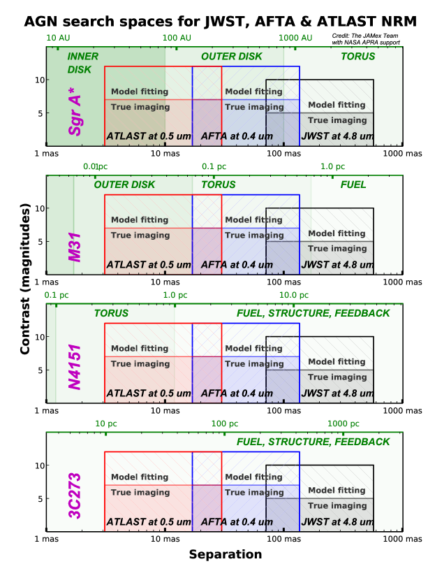
Figure 16.— Distance scales (and regions of AGNs) that can be investigated using space-based aperture masking interferometry, for four fiducial accreting SMBHs from Table 1. We assume luminosity distances of 16.9 Mpc and 749 Mpc to NGC 4151 and 3C 273 respectively. Characteristic distance scales are distinguished and shaded as follows: Relativistic innermost accretion disk within $<100r_{g}$, Keplerian meta-stable inner disk $10^{2}-10^{3}r_{g}$, outer disk $10^{3}-10^{4}r_{g}$, torus $10^{4}-10^{5}r_{g}$, region of AGN fuelling, feedback and binarity $>10^{5}r_{g}$. In each case we highlight the region of the galactic nucleus that could be probed by the three instruments in Table 1. For JWST-NIRISS AMI, the shaded region (‘true imaging’) corresponds to the imaging of extended structure at 5 mag pixel-to-pixel contrast ($10^{-2}$), surrounding a 7.5 mag point source, observed at 2 orientations for a total of 5.5 (3.5) min using F380M, F430M (F480M) filters. The unshaded NIRISS region (‘model fitting’) corresponds to the $5\sigma$ detection of a modeled binary at 10 mag contrast near a 7.5 mag central point source (Sivaramakrishnan et al., 2009a, 2010, 2012). The shaded regions for AFTA (at 400nm) and ATLAST (at 500nm) correspond to assumed achieveable pixel-to-pixel contrasts of 7 mag for extended structure, assuming photon noise dominates and extrapolating from JWST simulations. The unshaded AFTA and ATLAST regions correspond to the $5\sigma$ detection of a modeled binary at 12 mag constrast near a 7.5 mag central point source.

4.1. NGC 4151: archetypal Seyfert 1 AGN

NGC 4151 ($M_{\rm BH}\sim 1.3\times 10^{7}M_{\odot}$) is the archetypal Seyfert 1 AGN. NGC 4151 is bright ($\sim 10^{44}\rm{erg}\rm{s}^{-1}$ bolometric luminosity), nearby (16.9 Mpc), hosted in a weakly barred spiral galaxy (de Vaucouleurs et al., 1991), and is the most studied AGN at most wavelengths (e.g. Ulrich, 2000). The bar contains a total mass of $\sim 6\times 10^{8}M_{\odot}$ in HI, much of which is inflowing (Pedlar et al., 1993). A radio jet spans $4\arcsec$ either side of the nucleus and is misaligned by $\sim 25^{o}$ with the bar (Hutchings et al., 1998; Mundell et al., 2003). How the misalignment occurs, and the structure and dynamics of gas within $\sim 10$ pc (150 mas) remains unknown. Around $10^{9}M_{\odot}$ in gas lives within the central $\sim 900$ mas (60 pc) and $\sim 5\times 10^{7}M_{\odot}$ within the central $\sim 150$ mas (10 pc) (Winge et al., 1999). From mid-IR interferometric observations there is structure on scales of $2.0\pm 0.4$ pc ($\sim$30 mas) FWHM (Burtscher et al., 2009). However, this model-dependent estimate provides no information on geometry or clumpiness and insufficient size constraints. The structure could include part of the torus, or bars/spirals feeding the torus, or a warp from galactic plane to equatorial plane of the black hole (Bardeen & Petterson, 1975; King & Pringle, 2006). An AMI image (without priors) could distinguish between these scenarios and test models of feedback.

Assuming noise declines as $\sqrt{t}$, AMI imaging should probe complicated extended structure without prior modeling at a pixel-to-pixel contrast $\sim 10^{-3}$ in a $\sim 33(21)$ ks total exposure at two orientations, centered on $3.80,4.30,(4.80)\micron$. At these contrasts, NIRISS AMI can distinguish ordered fuelling structures from a disordered environment. Previous studies provide us with ‘priors’, which can guide our interpretation of blindly deconvolved images. For example, radio lobes at $\sim 200$ mas on either side of the NGC 4151 (right in the NIRISS search region), may coincide with shocks where the jet encounters interstellar medium (Mundell et al., 2003). If a coincidental structure shows up in an AMI image in the correct location and orientation, this radio prior enhances our ability to engage in physical interpretation. Additionally, short exposure ($\sim 2$ ks) NIRISS AMI observations, can test for the presence of symmetric extended structure (bars, torus, rings, spirals), via closure amplitude, down to a pixel-to-pixel contrast ratio of $10^{-4}$ at $5\sigma$ statistical significance.

4.2. 3C 273: The original quasar

3C 273 was the first quasar recognized to be extra-galactic (Schmidt, 1963), lying at $z=0.158$ (749 Mpc luminosity distance; $1\arcsec$=2.7 kpc linear scale) and is well studied at all wavelengths (e.g. Soldi et al., 2008). In most bands, the quasar core is saturated. So, modelling the underlying quasar environment and host galaxy requires PSF subtraction (e.g. Bahcall et al., 1995; Hutchings et al., 2004). Bahcall et al. (1997) find agreement with an underlying E4 host galaxy from fitting the residual intensity in regions $>1\arcsec$ after subtraction of a best-fit stellar PSF. However, any structure inside $1\arcsec$ will complicate both the subtraction of a stellar PSF and the model-dependent interpretation of the quasar host galaxy. The highest angular resolution study of 3C 273 to date was with the HST-ACS coronagraph (Martel et al., 2003), down to an IWA of 1300 mas. NIRISS AMI can probe a factor of 20 closer (75-600 mas) than the HST-ACS coronagraph (and a factor of 3 closer than coronagraphs on JWST). NIRISS AMI can test whether spiral structure at $\sim 1\arcsec$ which wraps around the quasar (Martel et al., 2003) continues inwards, possibly fuelling the quasar. NIRISS AMI can also test a merger origin for the quasar in departures from a smooth light profile at $<1\arcsec$. Once again, previous studies can provide ‘priors’ to guide deconvolution and physical interpretation. For example, Homan et al. (2001) measure the jet angle so structure that appears in a deconvolved image along the jet axis could be examined for a physical relationship to the jet.

4.3. M31: Nearby galactic nucleus

M31 at $\sim 0.8$ Mpc is the next nearest SMBH ($1.4\times 10^{8}M_{\odot}$) after Sgr A* but with less extinction along the sightline (Tempel et al., 2010). Within $3\arcsec$ ($\sim 10$ pc) of the center lies a double nuclear cluster of old red stars (Lauer et al., 1998). The double cluster is modeled as a projection effect of an eccentric disk of stars about $\sim 2$ pc in radius ($\sim 600$ mas) (Tremaine, 1995), which may be non-aligned with the M31 disk plane (Peiris & Tremaine, 2003). Inside the double cluster at $\sim 1$ pc ($\sim 300$ mas) lies a Keplerian disk of blue stars $\sim 100-200$ Myrs old (Bender et al., 2005; Lauer et al., 2012). The origin of both disks is unknown. Observations with NIRISS AMI can constrain the inclination angle and surface brightness of the eccentric disk which will help us understand its dynamical evolution, its origin and possibly its interaction with the inner Keplerian disk. For future missions, an IFU combined with AMI on a space telescope would also extract velocity dispersion information for the stellar disk.

5. Future missions: AFTA and ATLAST

NRM adds significant science impact to any proposed space telescope, for minor technical considerations (i.e. requiring detectors to be sampled at the resolution achievable with the mask, or pixellation of at least $\lambda/4D$). Future missions with AMI mode capabilities could probe regions deep in the potential well of SMBHs. For example, an NRM on ATLAST could image close to the event horizon of Sgr A* and could image to within a few hundred gravitational radii ($r_{g}=GM/c^{2}$) of nearby $\sim 10^{9}M_{\odot}$ Seyfert AGNs. ATLAST AMI could therefore be used to image whole AGN disks in the nearby Universe, allowing us to measure disk warps, gaps and cavities directly. From Table 1 and Fig. 16, we see that a 16 m ATLAST is significantly preferable to an 8m version, since it gives us most of the torus region in nearby Seyferts (IWA $\sim 10$ vs $\sim 20$ pc) and better access to the outer disk regions of some of the nearest SMBHs.

Figure 16 also shows the regions of several galactic nuclei that could be probed with AFTA. A 2.4 m space-based telescope used at optical and UV wavelengths ($\sim 400$nm) with an NRM, would probe different structures than JWST’s NIRISS AMI, particularly outer disk structure in nearby massive Seyfert AGNs. It could also investigate the connection between AGNs and star formation. For very large aperture future missions (e.g. a 16 m optical ATLAST), the additional collecting area would allow routine use of spectrometers in AMI mode. Simultaneous spectral information would help constrain the physical conditions and dynamics of imaged structures in AGNs–important for answers to many of the big questions outlined in §2. Sufficiently large collecting areas on future space telescopes would also permit us to image structures in polarized light from AGNs (Sivaramakrishnan et al., 2009b). Finally, while NIRISS AMI can expect to observe tens of AGNs, future missions could target hundreds.

6. Conclusions

Space-based aperture masking interferometry (AMI) can image extended structures around AGNs and quasars at moderate contrast and high angular resolution. Space-based imaging does not require a prior model of the target (we obtain fringe phase) unlike ground-based O/IR interferometry. O/IR interferometry also cannot obtain closure amplitudes from the ground, due to atmospheric instability. We demonstrate that a pixel-to-pixel contrast of $10^{-4}$ should be achieved in short exposures with JWST-NIRISS AMI, an order of magnitude better than obtainable with long exposure ground-based O/IR interferometry. JWST-NIRISS AMI will be a unique facility for carrying out moderate to high contrast observations of AGNs at high resolution, allowing us to constrain models of AGNs binarity, fuelling and structure at levels beyond present and proposed ground-based observatories. NRMs should be considered for addition to the filter wheel of most future space telescope missions, allowing high resolution and moderate to high contrast images of extended emission around bright sources in the optical/IR/UV bands.

Appendix A Non-redundant masking overview

We briefly review some relevant details of non-redundant masking (NRM) for observers unfamiliar with the technique. More complete descriptions of the technique can be found in Monnier (2003); Monnier & Allen (2013); Ireland (2013). We assume the Fraunhofer approximation of Fourier optics, viz., the image plane complex amplitude $a({\bf k})$ is the Fourier transform of the pupil plane complex amplitude $A({\bf x})$. In the monochromatic case, at wavelength $\lambda$, expressing pupil plane coordinates ${\bf x}\equiv(x,y)$ in units of the wavelength yields image plane coordinates ${\bf k}\equiv(k_{x},k_{y})$ in radians. We refer the reader to Bracewell (e.g., 2000) for details on Fourier theoretical results utilized in this section.

While our simulations have focussed on JWST-NIRISS’ 7-hole mask (Fig. 1), we describe NRM in more general terms here. $N_{h}$ identical holes in a pupil mask generate $N_{h}(N_{h}-1)/2$ sinusoidal fringes in the complex amplitude of the image plane. Each fringe is multiplied by an envelope function, the primary beam, which is the Fourier transform of the individual hole transmission function. The vector between a pair of holes in the mask is referred to as a baseline. The image intensity $I({\bf k})$ for the JWST-NIRISS 7-hole mask is shown in Fig. 3 (b and c). $I({\bf k})$ only contains spatial frequencies of the sky brightness distribution that are transmitted by the pupil mask. The complex visibility, $\mathcal{V}({\bf u})$, is the Fourier transform of the image intensity $I({\bf k})$. The domain of the complex visibility function is a pupil-like ‘spatial frequency’ space, with coordinates ${\bf u}\equiv(u,v)$. $\mathcal{V}({\bf u})$ is the Fourier component of the image brightness with spatial frequency ${\bf u}$. An inspection of the absolute value of $\mathcal{V}({\bf u})$ shows that only certain spatial frequencies pass through the mask (see Fig. 6). For a point source target, the quantity plotted in this figure is commonly known as the modulation transfer function (or MTF) of the optical system. Its support is obviously the region where the autocorrelation function of the pupil mask is non-zero. The isolated areas of signal in this plane, splodges (Lloyd et al., 2006), are twice as wide as the hole size. The centers of splodges are at the vector separations of the hole centers, i.e., the baselines. Since $I({\bf k})$ is real, $\mathcal{V}({\bf u})$ is Hermitian, so only one half of this space provides independent information. Thus, of the $7\times 6=42$ splodges in Fig. 6, only 21 are independent. By the so-called Fourier ‘DC’ theorem, $\mathcal{V}(\bf{0})$ is the energy in $I({\bf k})$ integrated over the entire image plane. Since no vector baselines in the pupil mask are repeated, each splodge is the result of only one baseline. It is this fact that enables unambiguous calibration of NRM images, since phase and amplitude errors in the incoming wavefront from a point source can be measured uniquely at each splodge. Fig. 7 shows the phase of the complex visibility. At ${\bf u}=\bf{0}$ the phase of $\mathcal{V}$ is zero, since $\mathcal{V}$ is a Hermitian function.

Appendix B The basics of image reconstruction

Correcting for pointing jitter: The variation of the pointing of a telescope during an exposure (jitter) leads to image smearing, as does the co-adding of short exposures. Image smearing will limit the accuracy of deconvolution (Fig. 5, left panels). However, a pointing offset ($\Delta{\bf k}$) generates a phase gradient across $\mathcal{V({\bf u}}$, as predicted by the Fourier Shift theorem. The gradient is proportional to $|\Delta{\bf k}|$, and is in the direction of $\Delta{\bf k}$. For example, in Fig. 7 the phase of $\mathcal{V({\bf u}})$ slopes in the 8 o’clock to 2 o’clock direction.

Under ideal conditions, without a pointing offset from the centroid of the image, the fringe phase is precisely the Fourier phase found by Fourier transforming the image. To align our images to sub-pixel accuracy (in order to remove the effects of jitter), we fit a plane to the measured phase of $\mathcal{V}({\bf u})$, making sure to constrain the constant term of the fit to zero. Subtracting the fitted phase gradient from the measured values of the phase of $\mathcal{V}$ is completely equivalent to sub-pixel alignment of the images. Since we utilize only fringe information in subsequent data reduction, we do not need to explicity reverse-transform our jitter-corrected $\mathcal{V(}{\bf u})$ to co-align our image data frames.

In practice we perform a Fast Fourier Transform, padding our incoming image data array by a factor of 4 to oversample $\mathcal{V}({\bf u})$ for convenience and clarity. We fit the phase of the complex visibility within square boxes $N\times N$ numerical pixels, centering the boxes on each splodge in the oversampled ${\bf u}$ plane. This fit is relatively insensitive to our choice of $N$, as long as $3<N<41$. We selected a value of $N=11$ for our data reduction. Including larger areas of the ${\bf u}$ plane ($N>40$) in the fit caused significant changes in the fit. We presume this is because these larger boxes mainly add noise to the fit.

Extraction: Ground-based optical, IR, and radio interferometry usually obtain a single complex visibility measurement per baseline. In the optical and IR, windowing the image plane data numerically leads to an averaging (by convolution with the Fourier transform of the windowing function) of $\mathcal{V}$ within a splodge. In radio this is due to instrumental implementation, with one signal (ignoring polariztion) measured by each antenna. (We note that array feeds on radio telescopes are beginning to change this paradigm). With one measurement per baseline, coverage in the ${\bf u}$ plane is sparse. Fig. 9a is equivalent to a ground-based 7 aperture array. In practice, baselines are moved by Earth’s rotation, which helps increase ${\bf u}$ plane coverage over time. Furthermore, the ‘zero-spacing’ complex visibility, $\mathcal{V}({\bf 0})$ is measured easily in these images. This is in contrast to most (but not all) radio interferometric measurements. Because space-based optical and IR imaging is stable and repeatable, one can obtain many more independent measurements of the complex visibility from a single image. This results in better instantaneous (u,v) coverage. We tried a few different approaches to improving our imaging algorithms by extracting more than one measurement per splodge.

Fig. 17 shows how different extraction patterns change the PSF and output clean model. Extracting samples of $\mathcal{V}$ too close to the edges of splodges adds more noise than signal (see Fig. 6). Our standard extraction pattern is a $31\times 31$ pixel box centered on each splodge. We read off values located at the bisectors and vertices of each extraction box. The optimal extraction pattern may be hexagonal, which would also allow simpler combination with some types of weighting (see Briggs, 1995, and below).

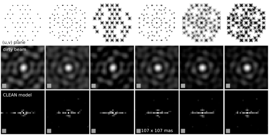
Figure 17.— Effect of different extraction patterns on image reconstruction. Each extraction pattern was used to reconstruct our fiducial model, shown in fig 4a. As the number of visibilities included increases, the number of artifacts decreases and the bar is more fully reconstructed.

Inversion: To inverse FT our phase corrected, extracted $\mathcal{V}$ and produce an image ($I^{\prime}_{\rm fringe}$–‘dirty map’) we choose: 1) a cell size $\delta$, i.e. the size of a resolution element in the image and 2) the size of $I^{\prime}_{\rm fringe}$. $\delta$ should be $\leq$ detector pixel scale (since information is available on at least these scales). We chose $\delta=0.25\lambda/D$ ($\sim 35.6$ mas). Reducing $\delta$ decreases the SNR per pixel, but optimal $\delta$ may be slightly smaller than our chosen value for some sources. The size of $I^{\prime}_{\rm fringe}$ must be large enough to prevent ringing, so we typically choose to match the original detector image size (or $256\times 256$ pixels, for $\delta\sim 35.6$ mas). Inverse FT potentially allows us to adjust the weighting of $\mathcal{V}$ to e.g. highlight structures at particular length scales in $I^{\prime}_{\rm fringe}$ (Briggs, 1995) by modulating amplitudes. For now we use natural weighting, but will investigate optimal weighting for various sources in future work.

Cleaning and restoration: Clean deconvolvers iteratively create a pixelated (gridded) model of the the spatial distribution of sky brightness (in the region observed). The algorithms place a delta function (clean component) at the ${\bf k}$ location of the brightest pixel in the fringe image $I^{\prime}_{\rm fringe}$, convolve it with the PSF and subtract the result from $I^{\prime}_{\rm fringe}$; repeating with next brightest pixel until some condition is met (number of iterations, no negative flux, etc.). The ‘gain’ parameter (we used gain=0.1) prevents oversubtracting on a single iteration. Because convolution and FT are linear operations, the sum of many delta functions seems a useful approximation of the sky. However, (some radio interferometrists will object) the true sky is not discretized in this way (Briggs, 1995). On the other hand, our (NIRISS) detector is pixelated, and so is our image of the sky. Therefore the clean model is one proper comparator for us. Thus, prior models of a source (where available) should be compared to clean models, in addition to the usual restored map.

We show clean models in conjunction with a restored map, $I_{R}=I^{\prime}_{\rm fringe}-(C*B)+(C*B_{R})$ (Taylor et al., 1999). Here $*$ denotes convolution, $I^{\prime}_{\rm fringe}$ is the fringe image, $C$ is the clean model, $B$ is the PSF or ‘dirty beam’ and $B_{R}$ is the ‘restoring beam’. We use a symmetric gaussian $B_{R}$ with a FWHM=71 mas ($0.5\lambda/D$). We also show a residual map, $R=I^{\prime}_{\rm fringe}-(C*B)$, in some cases. We can see that the restored map is just the clean model, smoothed to our theoretical angular resolution, plus the residuals–as such, it provides a conservative representation of the signifcance of reconstructed features in our images.

Appendix C Closure Phase & Closure Amplitude

Closure phase (CP) and closure amplitude (CA) are methods allowing calibration and removal of aperture-specific errors and uncorrelated atmospheric noise (e.g. Monnier & Allen, 2013, and references therein). CP assumes that phase errors are dominated by noise uncorrelated between apertures (e.g. small-scale atmospheric distortions or antenna-specific noise). For any closed triangle of apertures observing any source, such errors produce net zero displacement of phase (because the vector sum is zero). The CP is:

$$\Phi_{ijk}=\phi_{ij}+\phi_{jk}+\phi_{ki}$$ (C1)

where $\phi_{ij}$ is the phase measured along the baseline between apertures $i$ and $j$, etc. (and $\Phi_{ijk}=0$ for a point source). Given $N$ apertures, there are $N\choose 3$ closed triangles, but only ${N-1}\choose 2$ of these are independent (with $N\choose 2$ independent phases). CP is insensitive to phase errors which are correlated across apertures (which does occur in the atmosphere). Correlated errors cannot be calibrated out by CP; this is why ground-based O/IR interferometry cannot measure fringe phase.

CA is a similar technique, utilizing independent quads of apertures (e.g. Readhead et al., 1980). CA uses ratios of amplitudes along pairs of baselines, i.e. for apertures $i,j,k,l$ the CA is:

$$\Gamma_{ijkl}=\frac{A^{\prime}_{ij}A^{\prime}_{kl}}{A^{\prime}_{ik}A^{\prime}_{jl}}$$ (C2)

where $A^{\prime}_{ij}$ is the amplitude measured along the baseline between apertures $i$ and $j$, etc. There are $N(N-3)/2$ independent closure amplitudes. As long as $A_{ij}=g_{i}g^{*}_{j}A^{\prime}_{ij}$, where $A_{ij}$ is the true amplitude, $A^{\prime}_{ij}$ is the measured amplitude and $g_{i}$ and $g^{*}_{j}$ are the (uncorrelated) complex aperture specific gain and conjugate (and dominate the amplitude errors), the measured and true CAs are equal (and $\Gamma_{ijkl}=1$ for a point source). However, amplitudes in ground-based O/IR interferometry are dominated by correlated noise from the atmosphere so CA cannot be used (e.g. Monnier & Allen, 2013). Note also that the gain is an average over the entire aperture; when extracting $A^{\prime}$ away from the center of a splodge, we are effectively creating many subapertures. The gain for such subapertures is not clearly defined and does not have a simple relationship to the gain defined over the whole aperture. This is why it is mathematically incorrect to apply CP and CA relationships to visibilities extracted away from the splodge centers.

References

- Antonucci (1993) Antonucci, R. 1993, ARA&A, 31, 473
- Artymowicz et al. (1993) Artymowicz, P., Lin, D. N. C., & Wampler, E. J. 1993, ApJ, 409, 592
- Bahcall et al. (1997) Bahcall, J. N., Kirhakos, S., Saxe, D. H., & Schneider, D. P. 1997, ApJ, 479, 642
- Bahcall et al. (1995) Bahcall, J. N., Kirhakos, S., & Schneider, D. P. 1995, ApJ, 450, 486
- Baldwin et al. (1986) Baldwin, J. E., Haniff, C. A., Mackay, C. D., & Warner, P. J. 1986, Nature, 320, 595
- Bardeen & Petterson (1975) Bardeen, J. M., & Petterson, J. A. 1975, ApJ, 195, L65
- Baron et al. (2012) Baron, F., Cotton, W. D., Lawson, P. R., et al. 2012, in Society of Photo-Optical Instrumentation Engineers (SPIE) Conference Series, Vol. 8445, Society of Photo-Optical Instrumentation Engineers (SPIE) Conference Series
- Bender et al. (2005) Bender, R., Kormendy, J., Bower, G., et al. 2005, ApJ, 631, 280
- Bower et al. (2006) Bower, R. G., Benson, A. J., Malbon, R., et al. 2006, MNRAS, 370, 645
- Bracewell (2000) Bracewell, R. N. 2000, The Fourier transform and its applications
- Briggs (1995) Briggs, D. S. 1995, PhD thesis, New Mexico Institute of Mining and Technology, Socorro, New Mexico, 1995
- Burtscher et al. (2009) Burtscher, L., Jaffe, W., Raban, D., et al. 2009, ApJ, 705, L53
- Comerford et al. (2012) Comerford, J. M., Gerke, B. F., Stern, D., et al. 2012, ApJ, 753, 42
- Comerford et al. (2013) Comerford, J. M., Schluns, K., Greene, J. E., & Cool, R. J. 2013, ApJ, 777, 64
- de Vaucouleurs et al. (1991) de Vaucouleurs, G., de Vaucouleurs, A., Corwin, Jr., H. G., et al. 1991, Third Reference Catalogue of Bright Galaxies. Volume I: Explanations and references. Volume II: Data for galaxies between 0h and 12h. Volume III: Data for galaxies between 12h and 24h.
- Doyon et al. (2012) Doyon, R., Hutchings, J. B., Beaulieu, M., et al. 2012, in Society of Photo-Optical Instrumentation Engineers (SPIE) Conference Series, Vol. 8442, Society of Photo-Optical Instrumentation Engineers (SPIE) Conference Series
- Ferrarese & Merritt (2000) Ferrarese, L., & Merritt, D. 2000, ApJ, 539, L9
- Fried (1966) Fried, D. L. 1966, Journal of the Optical Society of America (1917-1983), 56, 1372
- Goodman & Rafikov (2001) Goodman, J., & Rafikov, R. R. 2001, ApJ, 552, 793
- Goodman & Tan (2004) Goodman, J., & Tan, J. C. 2004, ApJ, 608, 108
- Greenbaum et al. (2013) Greenbaum, A. Z., Sivaramakrishnan, A., & Pueyo, L. 2013, in Society of Photo-Optical Instrumentation Engineers (SPIE) Conference Series, Society of Photo-Optical Instrumentation Engineers (SPIE) Conference Series, submitted for publication
- Haniff et al. (1987) Haniff, C. A., Mackay, C. D., Titterington, D. J., Sivia, D., & Baldwin, J. E. 1987, Nature, 328, 694
- Ho (2008) Ho, L. C. 2008, ARA&A, 46, 475
- Högbom (1974) Högbom, J. A. 1974, A&AS, 15, 417
- Homan et al. (2001) Homan, D. C., Ojha, R., Wardle, J. F. C., et al. 2001, ApJ, 549, 840
- Hopkins & Hernquist (2006) Hopkins, P. F., & Hernquist, L. 2006, ApJS, 166, 1
- Hopkins & Quataert (2010) Hopkins, P. F., & Quataert, E. 2010, MNRAS, 407, 1529
- Hutchings et al. (2004) Hutchings, J. B., Stoesz, J., Veran, J.-P., & Rigaut, F. 2004, PASP, 116, 154
- Hutchings et al. (1998) Hutchings, J. B., Crenshaw, D. M., Kaiser, M. E., et al. 1998, ApJ, 492, L115
- Ireland (2013) Ireland, M. J. 2013, MNRAS, 433, 1718
- Ivanov et al. (1999) Ivanov, P. B., Papaloizou, J. C. B., & Polnarev, A. G. 1999, MNRAS, 307, 79
- Kauffmann & Heckman (2009) Kauffmann, G., & Heckman, T. M. 2009, MNRAS, 397, 135
- King & Pringle (2006) King, A. R., & Pringle, J. E. 2006, MNRAS, 373, L90
- Kocsis et al. (2012) Kocsis, B., Haiman, Z., & Loeb, A. 2012, MNRAS, 427, 2660
- Koekemor & Lindsay (2005) Koekemor, A. M., & Lindsay, K. 2005, in (Baltimore: STScI)
- Kormendy & Richstone (1995) Kormendy, J., & Richstone, D. 1995, ARA&A, 33, 581
- Krolik (1999) Krolik, J. H. 1999, Active galactic nuclei : from the central black hole to the galactic environment
- Lacour et al. (2011) Lacour, S., Tuthill, P., Amico, P., et al. 2011, A&A, 532, A72
- Lauer et al. (2012) Lauer, T. R., Bender, R., Kormendy, J., Rosenfield, P., & Green, R. F. 2012, ApJ, 745, 121
- Lauer et al. (1998) Lauer, T. R., Faber, S. M., Ajhar, E. A., Grillmair, C. J., & Scowen, P. A. 1998, AJ, 116, 2263
- Lawrence & Elvis (2010) Lawrence, A., & Elvis, M. 2010, ApJ, 714, 561
- Levin (2007) Levin, Y. 2007, MNRAS, 374, 515
- Lin & Papaloizou (1986) Lin, D. N. C., & Papaloizou, J. 1986, ApJ, 309, 846
- Liu et al. (2010) Liu, X., Greene, J. E., Shen, Y., & Strauss, M. A. 2010, ApJ, 715, L30
- Lloyd et al. (2006) Lloyd, J. P., Martinache, F., Ireland, M. J., et al. 2006, ApJ, 650, L131
- Martel et al. (2003) Martel, A. R., Ford, H. C., Tran, H. D., et al. 2003, AJ, 125, 2964
- Martini et al. (2003) Martini, P., Regan, M. W., Mulchaey, J. S., & Pogge, R. W. 2003, ApJ, 589, 774
- McCarthy et al. (2010) McCarthy, I. G., Schaye, J., Ponman, T. J., et al. 2010, MNRAS, 406, 822
- McKernan et al. (2014) McKernan, B., Ford, K. E. S., Kocsis, B., et al. 2014, MNRAS, submitted for publication
- McKernan et al. (2012) McKernan, B., Ford, K. E. S., Lyra, W., & Perets, H. B. 2012, MNRAS, 425, 460
- McKernan et al. (2011) McKernan, B., Ford, K. E. S., Lyra, W., et al. 2011, MNRAS, 417, L103
- McKernan et al. (2010a) McKernan, B., Ford, K. E. S., & Reynolds, C. S. 2010a, MNRAS, 407, 2399
- McKernan et al. (2010b) McKernan, B., Maller, A., & Ford, K. E. S. 2010b, ApJ, 718, L83
- McKernan & Yaqoob (1998) McKernan, B., & Yaqoob, T. 1998, ApJ, 501, L29
- McKernan et al. (2007) McKernan, B., Yaqoob, T., & Reynolds, C. S. 2007, MNRAS, 379, 1359
- Miniutti et al. (2010) Miniutti, G., Piconcelli, E., Bianchi, S., Vignali, C., & Bozzo, E. 2010, MNRAS, 401, 1315
- Monnier (2003) Monnier, J. D. 2003, Reports on Progress in Physics, 66, 789
- Monnier & Allen (2013) Monnier, J. D., & Allen, R. J. 2013, Radio and Optical Interferometry: Basic Observing Techniques and Data Analysis, ed. T. D. Oswalt & H. E. Bond, 325
- Mor et al. (2009) Mor, R., Netzer, H., & Elitzur, M. 2009, ApJ, 705, 298
- Mundell et al. (2003) Mundell, C. G., Wrobel, J. M., Pedlar, A., & Gallimore, J. F. 2003, ApJ, 583, 192
- Nenkova et al. (2008) Nenkova, M., Sirocky, M. M., Nikutta, R., Ivezić, Ž., & Elitzur, M. 2008, ApJ, 685, 160
- Pedlar et al. (1993) Pedlar, A., Kukula, M. J., Longley, D. P. T., et al. 1993, MNRAS, 263, 471
- Peiris & Tremaine (2003) Peiris, H. V., & Tremaine, S. 2003, ApJ, 599, 237
- Peterson et al. (2004) Peterson, B. M., Ferrarese, L., Gilbert, K. M., et al. 2004, ApJ, 613, 682
- Raban et al. (2009) Raban, D., Jaffe, W., Röttgering, H., Meisenheimer, K., & Tristram, K. R. W. 2009, MNRAS, 394, 1325
- Readhead et al. (1988) Readhead, A. C. S., Nakajima, T. S., Pearson, T. J., et al. 1988, AJ, 95, 1278
- Readhead et al. (1980) Readhead, A. C. S., Walker, R. C., Pearson, T. J., & Cohen, M. H. 1980, Nature, 285, 137
- Renard et al. (2011) Renard, S., Thiébaut, E., & Malbet, F. 2011, A&A, 533, A64
- Risaliti et al. (2002) Risaliti, G., Elvis, M., & Nicastro, F. 2002, ApJ, 571, 234
- Sault et al. (1995) Sault, R. J., Teuben, P. J., & Wright, M. C. H. 1995, in Astronomical Society of the Pacific Conference Series, Vol. 77, Astronomical Data Analysis Software and Systems IV, ed. R. A. Shaw, H. E. Payne, & J. J. E. Hayes, 433
- Schartmann et al. (2010) Schartmann, M., Burkert, A., Krause, M., et al. 2010, MNRAS, 403, 1801
- Schawinski et al. (2007) Schawinski, K., Thomas, D., Sarzi, M., et al. 2007, MNRAS, 382, 1415
- Schmidt (1963) Schmidt, M. 1963, Nature, 197, 1040
- Shakura & Sunyaev (1973) Shakura, N. I., & Sunyaev, R. A. 1973, A&A, 24, 337
- Shlosman & Begelman (1987) Shlosman, I., & Begelman, M. C. 1987, Nature, 329, 810
- Sijacki et al. (2007) Sijacki, D., Springel, V., Di Matteo, T., & Hernquist, L. 2007, MNRAS, 380, 877
- Silk & Nusser (2010) Silk, J., & Nusser, A. 2010, ApJ, 725, 556
- Sirko & Goodman (2003) Sirko, E., & Goodman, J. 2003, MNRAS, 341, 501
- Sivaramakrishnan et al. (2009a) Sivaramakrishnan, A., Tuthill, P. G., Ireland, M. J., et al. 2009a, in Society of Photo-Optical Instrumentation Engineers (SPIE) Conference Series, Vol. 7440, Society of Photo-Optical Instrumentation Engineers (SPIE) Conference Series
- Sivaramakrishnan et al. (2009b) Sivaramakrishnan, A., Tuthill, P., Martinache, F., et al. 2009b, in Astronomy, Vol. 2010, astro2010: The Astronomy and Astrophysics Decadal Survey, 40
- Sivaramakrishnan et al. (2010) Sivaramakrishnan, A., Lafrenière, D., Tuthill, P. G., et al. 2010, in Society of Photo-Optical Instrumentation Engineers (SPIE) Conference Series, Vol. 7731, Society of Photo-Optical Instrumentation Engineers (SPIE) Conference Series
- Sivaramakrishnan et al. (2012) Sivaramakrishnan, A., Lafrenière, D., Ford, K. E. S., et al. 2012, in Society of Photo-Optical Instrumentation Engineers (SPIE) Conference Series, Vol. 8442, Society of Photo-Optical Instrumentation Engineers (SPIE) Conference Series
- Soldi et al. (2008) Soldi, S., Türler, M., Paltani, S., et al. 2008, A&A, 486, 411
- Springel et al. (2006) Springel, V., Frenk, C. S., & White, S. D. M. 2006, Nature, 440, 1137
- Springel et al. (2005) Springel, V., White, S. D. M., Jenkins, A., et al. 2005, Nature, 435, 629
- Syer & Clarke (1995) Syer, D., & Clarke, C. J. 1995, MNRAS, 277, 758
- Taylor et al. (1999) Taylor, G. B., Carilli, C. L., & Perley, R. A., eds. 1999, Astronomical Society of the Pacific Conference Series, Vol. 180, Synthesis Imaging in Radio Astronomy II
- Tempel et al. (2010) Tempel, E., Tamm, A., & Tenjes, P. 2010, A&A, 509, A91
- Tremaine (1995) Tremaine, S. 1995, AJ, 110, 628
- Turner & Miller (2009) Turner, T. J., & Miller, L. 2009, A&A Rev., 17, 47
- Tuthill et al. (1998) Tuthill, P. G., Monnier, J. D., Danchi, W. C., & Haniff, C. A. 1998, in Society of Photo-Optical Instrumentation Engineers (SPIE) Conference Series, Vol. 3350, Astronomical Interferometry, ed. R. D. Reasenberg, 839–846
- Tuthill et al. (2000) Tuthill, P. G., Monnier, J. D., Danchi, W. C., Wishnow, E. H., & Haniff, C. A. 2000, PASP, 112, 555
- Ulrich (2000) Ulrich, M.-H. 2000, A&A Rev., 10, 135
- Urry & Padovani (1995) Urry, C. M., & Padovani, P. 1995, PASP, 107, 803
- Volonteri et al. (2007) Volonteri, M., Sikora, M., & Lasota, J.-P. 2007, ApJ, 667, 704
- Weedman & Houck (2009) Weedman, D. W., & Houck, J. R. 2009, ApJ, 698, 1682
- Winge et al. (1999) Winge, C., Axon, D. J., Macchetto, F. D., Capetti, A., & Marconi, A. 1999, ApJ, 519, 134