Quantum Entanglement of Local Operators in Conformal Field Theories
Masahiro Nozakia, Tokiro Numasawaa and Tadashi Takayanagia,baYukawa Institute for Theoretical Physics,
Kyoto University,
Kitashirakawa Oiwakecho, Sakyo-ku, Kyoto 606-8502, Japan
bKavli Institute for the Physics and Mathematics
of the Universe,
University of Tokyo, Kashiwa, Chiba 277-8582, Japan
Abstract
We introduce a series of quantities which characterizes a given local operator in any conformal field theory from the viewpoint of quantum entanglement. It is defined by the increased amount of (Renyi) entanglement entropy at late time for an excited state defined by acting the local operator on the vacuum. We consider a conformal field theory on an infinite space and take the subsystem in the definition of the entanglement entropy to be its half. We calculate these quantities for a free massless scalar field theory in and dimensions. We find that these results are interpreted in terms of quantum entanglement of finite number of states, including EPR states. They agree with a heuristic picture of propagations of entangled particles.
1. Introduction
Recently entanglement entropy has become a center of wide interest in a broad array of theoretical physics researches. It is defined as the von-Neumann entropy of the reduced density matrix
for a subsystem . It has been used as a useful quantity which characterizes quantum properties of ground states in condensed matter physics (see e.g.capro ; wen ).
Moreover, it is intriguing to apply entanglement entropy to quantify excited states. For excited states in conformal field theories (CFTs), it was shown that entanglement entropy has an interesting property analogous to the first law of thermodynamics if the size of subsystem is much smaller than the excitation scale. This property was derived in thm from the holographic entanglement entropy RT and later a field theoretic derivation was given in BCHM . Refer also to UAM for an earlier related result.
Consider a CFT on a sphere times the time axis and pick up an excited state defined by acting a local operator on the vacuum state . Then the first law argues that the increased amount of entanglement entropy for this excited state, is essentially given by the conformal dimension of the operator if the subsystem size (or equally the excitation energy) is very small.
On the other hand, it is natural to ask what will happen if we consider in the opposite limit i.e. the large size limit of subsystem . One may expect that we get another basic quantity of an operator in CFTs which can be as fundamental as the conformal dimension. The main aim of this letter is to make a first step to answer this question. As we will see, this new quantity characterizes the quantum entanglement of an operator itself, together with its Rnyi entropic versions.
There have been extensive studies on time evolutions of entanglement entropy in certain classes of largely excited states, called quantum quenches. One of them is called a global quench, which is triggered by changing parameters homogeneously cag and is a special example of thermalization. Another class is called a local quench, which occurs by changing Hamiltonian locally cal ; eis .
2. (Rnyi) Entropy for locally Excited States
In this letter we focus on excited states which are defined by acting a local operators on the vacuum with a finite and positive conformal dimension in a given CFT. We consider a conformal field theory in the dimensional Euclidean space , whose coordinates are
denoted by . The density matrix for the total system is given by
and we choose the excited state by acting an operator as follows
(1)
where is a normalization factor such that .
The constant becomes finite after a proper regularization as we will explain later.
Our state
cannot be treated as a small perturbation from the vacuum state, though it describes an excited state much milder than that in local and global quantum quenches. Define also the ground state density matrix as .
To define the entanglement entropy, we choose the subsystem to be a half of the total space i.e. . The reduced density matrix is defined by , tracing out the complement of , called the subsystem . The Rnyi entanglement entropy is defined by
(2)
The limit coincides with the entanglement entropy . The difference of between an excited state and the ground state is defined to be .
We first calculate the entropies in the Euclidean formulation and finally perform an analytical continuation to see the dependence on the real time . The time-evolution of density matrix is described by
(3)
where we defined .
An infinitesimal parameter is an ultraviolet regularization.
In general, shows a non-trivial time-evolution.
Our analysis of explicit examples suggests that are monotonically increasing with the time for any local operator . Moreover, they finally approach to certain finite values in the late time limit . These values depend on the choice of local operator and are the quantities of our main interest.
To calculate , we employ the path-integral formalism by extending the replica method analysis in capro for ground states. We can express
Tr in terms of partition functions as Tr. The partition on , corresponding to , is written as
, while is the partition function on -sheeted space with
s inserted (see Fig.1). It is also useful to define the vacuum partition functions on and by and , respectively, so that we have Tr for the ground state.
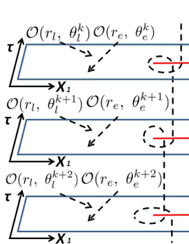
Figure 1: The -sheeted geometry is constructed by gluing the upper cut along subsystem A on a sheet to the lower cut on the next sheet.
In this way, we find that is rewritten as
(4)
The term in the second line is given by a points correlation function of on . The final term is a two point function of on . The values of
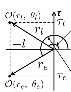
and are determined as follows. First we introduced the polar coordinate as . The angular coordinate takes values on (see Fig.2). We set at each location of and this measures the distance between the excited point and the boundary of the subsystem . Since our calculations do not depend on locations in other directions , we omit their dependence. By defining , the locations of the insertions are given by .
Figure 2: The Euclidean coordinate and operator insertions.
3. Results in Free Scalar Field Theories
To obtain analytical results of , we focus on a free massless scalar field theory defined by the familiar action
. We performed explicit calculations for various operators and replica numbers in 2, 4 and 6 dimension. We found that the results of late time values do not depend on the dimension as long as the dimension is higher than two as we summarized in Table I. In two dimension, we will present results separately soon later. In this letter we will skip the details of the calculations because they are straightforward (but tedious) computations, employing the
Green functions on in dow ; sac . Rather we give a brief summary of our results below. Refer also to the appendix A for Green functions and appendix B for some examples of entropy computations.
Table 1: and for free massless scalar field theories in dimensions higher than two ().
Four and Six Dimensional Results
First we describe the results in and dimensional case. As a series of local operators, we consider the primary operators
(5)
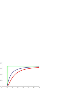
The time-evolutions of the Rnyi entropies are all similar. In general, are vanishing in the region . They start increasing at and keep to increase in the region . Finally, they approach to certain constant values , in the late time limit .
For example, the Rnyi entropies for the operator (i.e. ) in and dimension are given as follows when , in the limit (see Fig.3)
(6)
(7)
Thus we find .
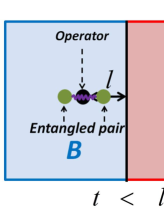
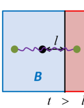
We can interpret this behavior as follows. Firstly, an entangled pair of two quanta is produced at the point where the local operator is inserted as in Fig.4. And each of the two propagates in the opposite directions at the speed of light. When one of them reaches the boundary of the region A, the entanglement between two quanta starts to contribute to the (Rnyi) entanglement entropies between A and B. Thus the minimum time for this event is and generally it takes more than for a pair moving in a generic direction. Finally, the entropies approach to certain constants as the two quanta remain to stay in and , respectively, forever. This consideration also explains the monotonicity of entropy under time-evolutions.
In the above, we did not take into account the conformal mass term of scalar field theory, where is the scalar curvature. Even though in general this affects results for excited states as noted in LM , our results in the limit do not change by this effect.
Figure 3:
The plots of as functions of in the limit . We chose . The red and blue curve correspond to the operator () in 6 and 4 dimension, respectively. The green graph describes the entropy for the operator in 2 dimension.
Figure 4: This shows a schematic explanation for the time evolution of in terms of entangled pairs.
An Interpretation in terms of entangled pairs
We calculated the late time values for with
various and we summarized them in Table I. Interestingly, we can find that are equal to the values of Rnyi entropies for dimensional Hilbert spaces under a simple rule. Indeed, let us define a reduced density matrix by the following diagonal matrix
(8)
where . Then we can confirm
(9)
The Rnyi entropy can be explicitly written as
(10)
Taking the limit leads to the entanglement entropy
(11)
Now we would like to provide an interpretation of the density matrices (8) in terms of
the entangled pairs. We decompose the scalar field as , where and describe the modes which are moving toward the left () and right () direction. The key observation is that the late time entanglement entropy measures the entanglement between the left and right as is defined by . We can expand our excited states as follows
(12)
where are normalized such that . Indeed, we can confirm that (12) leads to the density matrix (8) after tracing out right-moving sector.
Especially, if we choose , (12) is equivalent to the maximally entangled
two spins (i.e. EPR state). Thus we find for any .
It might also be useful to notice that for we find the simple formula
(13)
Two dimensional Results
Finally, we describe the results for the two dimensional free massless scalar.
As opposed to higher dimensions, the operators (5) cannot be regarded as local operators in our sense as their conformal dimensions are vanishing.
This motivates us to choose the following primary operators for any real values of
(14)
By explicit calculations, it is easy to show that and are always vanishing for the operator . On the other hand, if we consider the operator
, we obtain the following result
(15)
Again we can explain these results in terms of the entangled pairs. In two dimension, we can exactly decompose the scalar field into left and right-moving mode as . Then it is obvious that the excited state is a direct product state and should have the vanishing quantum entanglement. On the other hand,
(16)
is the EPR state and has the entropy for any . Moreover, since in two dimension, the light-like motion of entangled pair is one dimensional and this is the reason why the entropy instantaneously jumps at as opposed to the results in higher dimensions (see Fig.3). It is curious to note that the results do not depend on the parameter or equally the conformal dimension.
The results for other local operators can be similarly understood in terms of the entangled pairs. For example, consider operators of the form , where and
are arbitrary chiral and anti-chiral local operators such as
, where and are the derivatives with respect to and . If we act these states on the vacuum , it is obvious that they are all direct product states between left and right-moving sector. Therefore and are all vanishing when we take the cut off to be vanishing.
4. Conclusions
In this letter, we proposed a series of new quantities
which characterizes local operators in CFTs. In short, they measure the amount quantum entanglement of an operator or more intuitively quantum mechanical degrees of freedom included in an operator.
They are defined as the increased amount of
-th Rnyi entanglement entropy at late time considering a
time-evolution of an excited state obtained by acting an operator on the vacuum. We chose the subsystem to be a half of the total space . We conjectured that are monotonically increasing functions of time.
We analyzed various explicit examples in free massless scalar field theories in and dimension. They are enough to draw general conclusions for free massless scalar theories
in dimension higher than two, as summarized in Table I. We found that all of our results, even including two dimensional ones, can be understood in terms of quantum entanglement in finite dimensional Hilbert spaces like qubits in quantum information theory.
The behavior of can be understood in terms of relativistic propagations of entangled pairs created by local operators. Indeed, the entropy starts increasing just when one of the entangled pair reaches the boundary of subsystem . The time-evolution of entropy becomes step-functional in two dimension, while it gets a smooth function in higher dimension. This is because there are many directions to propagate and the arrival time at depends on directions in the latter.
Note that taking the subsystem to be infinitely large is important to obtain a non-zero constant entropy at late time. Our entangled pair interpretation suggests that the late time values do not change even if we modify the shape of continuously. In this sense, they are topological quantities.
It is an interesting future problem to see how our results are changed in interacting CFTs, where our entangled quasi-particle interpretation might be modified. We may think of holographic computations similar to NNT . It will also be intriguing to generalize our arguments to massive quantum field theories.
Acknowledgements We thank J. Bhattacharya, S. He,
T. Nishioka, S. Ryu, N. Shiba and T. Ugajin for useful
discussions. TT is supported by JSPS Grant-in-Aid for Scientific
Research (B) No.25287058 and JSPS Grant-in-Aid for Challenging
Exploratory Research No.24654057. TT is also supported by World Premier
International Research Center Initiative (WPI Initiative) from the
Japan Ministry of Education, Culture, Sports, Science and Technology
(MEXT).
References
(1)
A. Kitaev and J. Preskill,
Phys. Rev. Lett. 96, 110404 (2006)
[arXiv:hep-th/0510092];
M. Levin and X. G. Wen,
Phys. Rev. Lett. 96, 110405 (2006)
[arXiv:cond-mat/0510613].
(2)
P. Calabrese and J. L. Cardy,
J. Stat. Mech. 0406, P06002 (2004)
[hep-th/0405152].
(3)
J. Bhattacharya, M. Nozaki, T. Takayanagi and T. Ugajin,
Phys. Rev. Lett. 110, no. 9, 091602 (2013)
[arXiv:1212.1164].
(4)
S.Ryu and T.Takayanagi,Phys.Rev.Lett.96(2006)181602
[hep-th/0603001];JHEP0608045(2006)[hep-th/0605073].
(5)
D. D. Blanco, H. Casini, L. -Y. Hung and R. C. Myers,
JHEP 1308, 060 (2013)
[arXiv:1305.3182 [hep-th]];
G. Wong, I. Klich, L. A. Pando Zayas and D. Vaman,
arXiv:1305.3291 [hep-th].
(6)
F. C. Alcaraz, M. I. Berganza, G. Sierra,
Phys. Rev. Lett. 106 (2011) 201601 [arXiv:1101.2881 [cond-mat]].
(7)
P. Calabrese and J. L. Cardy,
J. Stat. Mech. 04 (2005) P04010, cond-mat/0503393.
(8)
P. Calabrese and J. L. Cardy,
J. Stat. Mech. 0710 (2007) P10004, arXiv:0708.3750.
(9) V. Eisler and I. Peschel, J. Stat. Mech. 0706 (2007) P06005, [cond-mat/0703379 [cond-mat.stat-mech]]
(10)
J. S. Dowker,
J. Phys. A 10, 115 (1977);
S. Deser and R. Jackiw,
Commun. Math. Phys. 118, 495 (1988);
M. E. X. Guimaraes and B. Linet,
Commun. Math. Phys. 165, 297 (1994).
(11) Metlitski, Max A. Fuertes, Carlos A. and Sachdev, Subir
Phys.Rev.B.80,115122(2009)
[hep-th/0904.4477].
(13)
M. Nozaki, T. Numasawa and T. Takayanagi,
JHEP 1305 (2013) 080 [arXiv:1302.5703 [hep-th]]; T. Ugajin,
arXiv:1311.2562 [hep-th].
Appendix A Appendix A: Propagators in n-sheeted space
We would like to compute Rnyi entanglement entropies for locally excited states.
Then we have to construct propagators on an Euclidean space which has a conical singularity.
Below we consider the massless free scalar field theory on -sheeted space in even dimensions. The shape of subsystem is chosen to be a half of the total space (see Fig.5). We introduce the polar coordinate as .
Figure 5: The subsystem A is defined by the region . Operators are inserted into the points .
The Green function is defined by
(17)
where .
Then we can expand the Green function by the eingenfunctions ,
(18)
where .
As in capro , the Green function can be expressed as
(19)
where and is the Bessel function of the first kind.
By using a Schwinger parameter, the denominator of (19) can be expressed as
(20)
We can integrate with respect to ,
(21)
When we use the formula of Bessel function, the integral of from to in (19) can be performed,
(22)
where is the modified Bessel function of first kind.
And is expressed as
(23)
After integrating with respect to , can be expressed as
(24)
When is odd, we can integrate with respect to . When is , is given by