Single Higgs boson production at $e^{+}e^{-}$ colliders in the Littlest Higgs Model with T-parity

Abstract

In this work, we investigate the Higgs-boson production processes $e^{+}e^{-}\rightarrow ZH$, $e^{+}e^{-}\rightarrow\nu_{e}\bar{\nu_{e}}H$ and $e^{+}e^{-}\rightarrow e^{+}e^{-}H$ in the littlest Higgs model with T-parity. We present the production cross sections, the relative corrections and some distributions of the final states. In the allowed parameter space, we find that the relative corrections of the three production channels are negative, the relative correction of the $ZH$ production can reach $-7.5\%$ and the relative corrections of the $\nu_{e}\bar{\nu_{e}}H$ and $e^{+}e^{-}H$ production can both reach $-6.5\%$ for $\sqrt{s}=500$ GeV with the scale $f=$694 GeV.

I Introduction

In the Standard Model (SM)sm , the Higgs mechanismHiggs mechanism leads to the prediction of the Higgs boson. The Higgs boson is an excitation of the Higgs field, which is an essential ingredient and will provide direct evidence for the mechanism of spontaneous symmetry breaking. The SM without the Higgs boson is incomplete since it predicts massless fermions and gauge bosons. However, the direct detection of Higgs boson is difficult because it couples most strongly to the heaviest available channels which will cascade into complicated multiparticle final states. On the 4th of July 2012, after a long wait and even generations of immense efforts by thousands of scientists, CERN announced that both the ATLASATLAS and CMSCMS experiments had discovered a new Higgs-like boson, which was a historical event for high-energy physics.

The Large Hadron Collider(LHC) experiments will determine various properties of the Higgs boson, up to now, most measurements of this new particle are consistent with the SM prediction. This corners the new physics that affects the Higgs couplings to a decoupling region higgscoupling . Due to the clean environment, the complete profile of the Higgs boson can be precisely studied at an electron-positron linear colliderhiggsee . In $e^{+}e^{-}$ collider, there are two main production mechanisms for the SM Higgs boson: Higgs-strahlung and $WW$-fusion. Compared with $WW$-fusion, the cross section for the similar $ZZ$-fusion process is suppressed by one order of magnitude. These processes have been studied at $e^{+}e^{-}$, $e\gamma$ and $\gamma\gamma$ modes in the context of the SMzhsm and the new physics modelszhnp .

As an extension of the SM, the littlest Higgs model with T-parity(LHT)LHT can successfully solve the electroweak hierarchy problem and so far remains a popular candidate of new physics. In the LHT model, some new particles are predicted and some SM couplings are modified so that the Higgs properties may deviate from the SM Higgs boson. So the Higgs-boson production processes are ideal ways to probe the LHT model at the high energy colliders. These production processes in the LHT model have been studied at the LHCHiggsLHC , but have not been calcualted at the $e^{+}e^{-}$ colliders. In this work, we will study the single Higgs production processes, $e^{+}e^{-}\rightarrow ZH$, $e^{+}e^{-}\rightarrow\nu_{e}\bar{\nu_{e}}H$ and $e^{+}e^{-}\rightarrow e^{+}e^{-}H$, in the LHT model at the $e^{+}e^{-}$ collider.

The paper is organized as follows. In Sec.II we give a brief review of the LHT model related to our work. In Sec.III we study the effects of the LHT model in the single Higgs boson production and present some discussions of numerical results. Finally, we give a short summary in Sec.IV.

II A brief review of the LHT model

In this section, we only review the LHT model related to our calculations. For more details, one can refer to Refs.LHTphy .

The LHT model was based on a non-linear $\sigma$ model describing an $SU(5)/SO(5)$ symmetry breaking, with the global group $SU(5)$ being spontaneously broken into $SO(5)$ by a $5\times 5$ symmetric tensor at the scale $f\sim\mathcal{O}$(TeV).

An $[SU(2)\times U(1)]_{1}\times[SU(2)\times U(1)]_{2}$ subgroup of the $SU(5)$ is gauged and the gauge fields $W_{i\mu}^{a}$ and $B_{i\mu}$ $(a=1,2,3,~{}i=1,2)$ are introduced. In this model, the action of T-parity on the gauge fields and scalar sector are defined as:

$$W_{1\mu}^{a}\longleftrightarrow W_{2\mu}^{a},~{}~{}~{}~{}B_{1\mu}\longleftrightarrow B_{2\mu},~{}~{}~{}~{}\Pi\longrightarrow-\Omega\Pi\Omega,$$ (1)

where $\Omega={\rm diag}(1,1,-1,1,1)$. The T-odd and T-even gauge fields can be obtained as

$$W_{L}^{a} = \frac{W_{1}^{a}+W_{2}^{a}}{\sqrt{2}},~{}~{}~{}B_{L}=\frac{B_{1}+B_{2}}{\sqrt{2}},~{}~{}~{}~{}~{}(\mbox{T-even}),$$

$$W_{H}^{a} = \frac{W_{1}^{a}-W_{2}^{a}}{\sqrt{2}},~{}~{}~{}B_{H}=\frac{B_{1}-B_{2}}{\sqrt{2}},~{}~{}~{}~{}~{}(\mbox{T-odd}).$$ (2)

The electroweak symmetry breaking $SU(2)_{L}\times U(1)_{Y}\to U(1)_{em}$ takes place via the usual Higgs mechanism. The mass eigenstates of the gauge fields are given by

$$W_{L}^{\pm}=\frac{W_{L}^{1}\mp iW_{L}^{2}}{\sqrt{2}},~{}~{}~{}~{}\left(\begin{array}[]{c}A_{L}\\ Z_{L}\end{array}\right)=\left(\begin{array}[]{rc}\cos\theta_{W}&\sin\theta_{W}\\ -\sin\theta_{W}&\cos\theta_{W}\end{array}\right)\left(\begin{array}[]{c}B_{L}\\ W_{L}^{3}\end{array}\right),~{}~{}~{}~{}(\mbox{T-even}),$$ (9)

$$W_{H}^{\pm}=\frac{W_{H}^{1}\mp iW_{H}^{2}}{\sqrt{2}},~{}~{}~{}\left(\begin{array}[]{c}A_{H}\\ Z_{H}\end{array}\right)=\left(\begin{array}[]{cr}\cos\theta_{H}&-\sin\theta_{H}\\ \sin\theta_{H}&\cos\theta_{H}\end{array}\right)\left(\begin{array}[]{c}B_{H}\\ W_{H}^{3}\end{array}\right),~{}~{}~{}~{}(\mbox{T-odd}),$$ (16)

where $\theta_{W}$ is the usual Weinberg angle and $\theta_{H}$ is the mixing angle defined by

$$\sin{\theta_{H}}\simeq\frac{5gg^{\prime}}{4(5g^{2}-g^{\prime 2})}\frac{v_{SM}^{2}}{f^{2}},$$ (17)

where $v_{SM}\simeq 246$ GeV is the SM Higgs vacuum expectation value (VEV).

To implement T-parity in the fermion sector, it requires the introduction of the mirror fermions. For each SM $SU(2)_{L}$ doublet, under the $SU(2)_{1}\times SU(2)_{2}$ gauge symmetry, a doublet under $SU(2)_{1}$ and one under $SU(2)_{2}$ are introduced. The T-parity even combination is associated with the SM $SU(2)_{L}$ doublet while the T-odd combination is given a $\mathcal{O}(f)$ mass.

In order to avoid dangerous contributions to the Higgs mass from one-loop quadratic divergences, the third generation Yukawa sector must be modified. One must also introduce additional singlets $t^{\prime}_{1R}$ and $t^{\prime}_{2R}$ which transform under T-parity as

$$t^{\prime}_{1R}\leftrightarrow-t^{\prime}_{2R}$$ (18)

so the top sector masses can be generated in the following T-parity invariant way

$$\mathcal{L}_{top} = -\frac{1}{2\sqrt{2}}\lambda_{1}f\epsilon_{ijk}\epsilon_{xy}\big{[}(\bar{Q}_{1})_{i}(\Sigma)_{jx}(\Sigma)_{ky}-(\bar{Q}_{2}\Sigma_{0})_{i}(\tilde{\Sigma})_{jx}(\tilde{\Sigma})_{ky}\big{]}u_{3R}$$ (19)

$$- \lambda_{2}f(\bar{t}^{\prime}_{1}t^{\prime}_{1R}+\bar{t}^{\prime}_{2}t^{\prime}_{2R})+h.c.$$

For the other quarks, it will not be necessary to modify the Yukawa Lagrangian as in the top sector since their Yukawa coupling is at least one order of magnitude smaller. Therefore we do not need to introduce additional singlets for the remaining up-type quarks and the Yukawa coupling is accordingly given by

$$\mathcal{L}_{up}=-\frac{1}{2\sqrt{2}}\lambda_{u}f\epsilon_{ijk}\epsilon_{xy}\left[(\bar{Q}_{1})_{i}(\Sigma)_{jx}(\Sigma)_{ky}-(\bar{Q}_{2}\Sigma_{0})_{i}(\tilde{\Sigma})_{jx}(\tilde{\Sigma})_{ky}\right]u_{R}+h.c.$$ (20)

For the down-type quarks, we can construct the Yukawa interaction to give them masses in the following way:

$$\mathcal{L}_{down}=\frac{i\lambda_{d}}{2\sqrt{2}}f\epsilon_{ij}\epsilon_{xyz}\left[(\bar{\Psi}_{2})_{x}(\Sigma)_{iy}(\Sigma)_{jz}X-(\bar{\Psi}_{1}\Sigma_{0})_{x}(\tilde{\Sigma})_{iy}(\tilde{\Sigma})_{jz}\tilde{X}\right]d_{R}+h.c.\$$ (21)

In our calculations, the $Hb\bar{b},HZZ$ and $HWW$ coupling involved will be different from the SM coupling, which are given by

$$V_{Hb\bar{b}} = -\frac{m_{b}}{v}(1-\frac{1}{6}\frac{v^{2}}{f^{2}}),$$ (22)

$$V_{HZ_{\mu}Z_{\nu}} = \frac{2m_{Z}^{2}}{v}(1-\frac{1}{6}\frac{v^{2}}{f^{2}})g_{\mu\nu},$$ (23)

$$V_{HW_{\mu}W_{\nu}} = \frac{2m_{W}^{2}}{v}(1-\frac{1}{6}\frac{v^{2}}{f^{2}})g_{\mu\nu},$$ (24)

where $v=v_{SM}(1+\frac{1}{12}\frac{v_{SM}^{2}}{f^{2}})$. Although the differences occur at the order $\mathcal{O}(v^{2}/f^{2})$, their contributions cannot be ignored because they appear at the lowest-order.

III Calculation and Numerical results

In the LHT model, the lowest-order Feynman diagrams of the process $e^{+}e^{-}\rightarrow ZH$, $e^{+}e^{-}\rightarrow\nu_{e}\bar{\nu_{e}}H$ and $e^{+}e^{-}\rightarrow e^{+}e^{-}H$ are shown in Fig.1. We can see that the tree-level Feynman diagrams of these processes in the LHT model are identical with that in the SM.

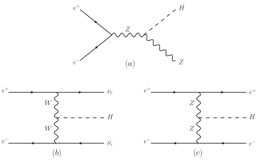
Figure 1: Lowest-order Feynman diagrams for $e^{+}e^{-}\rightarrow ZH$(a), $e^{+}e^{-}\rightarrow\nu_{e}\bar{\nu_{e}}H$(b) and $e^{+}e^{-}\rightarrow e^{+}e^{-}H$(c).

In our numerical calculations, the SM parameters are taken as followsparameters

$$G_{F}=1.16637\times 10^{-5}{\rm GeV}^{-2},~{}\sin^{2}\theta_{W}=0.231,~{}\alpha_{e}=1/128,$$

$$m_{b}=4.65{\rm GeV},~{}m_{Z}=91.1876{\rm GeV},~{}m_{H}=126{\rm GeV},$$ (25)

$$m_{e}=0.51{\rm MeV},~{}m_{\mu}=105.66{\rm MeV},~{}m_{\tau}=1776.82{\rm MeV}.$$ (26)

There is only one LHT parameter, the breaking scale $f$, in our calculation. Considering the constraints in Refs.constraints , we choose the relatively relaxed parameter space and vary the scale in the range $500$ GeV$\leq f\leq 1500$ GeV.

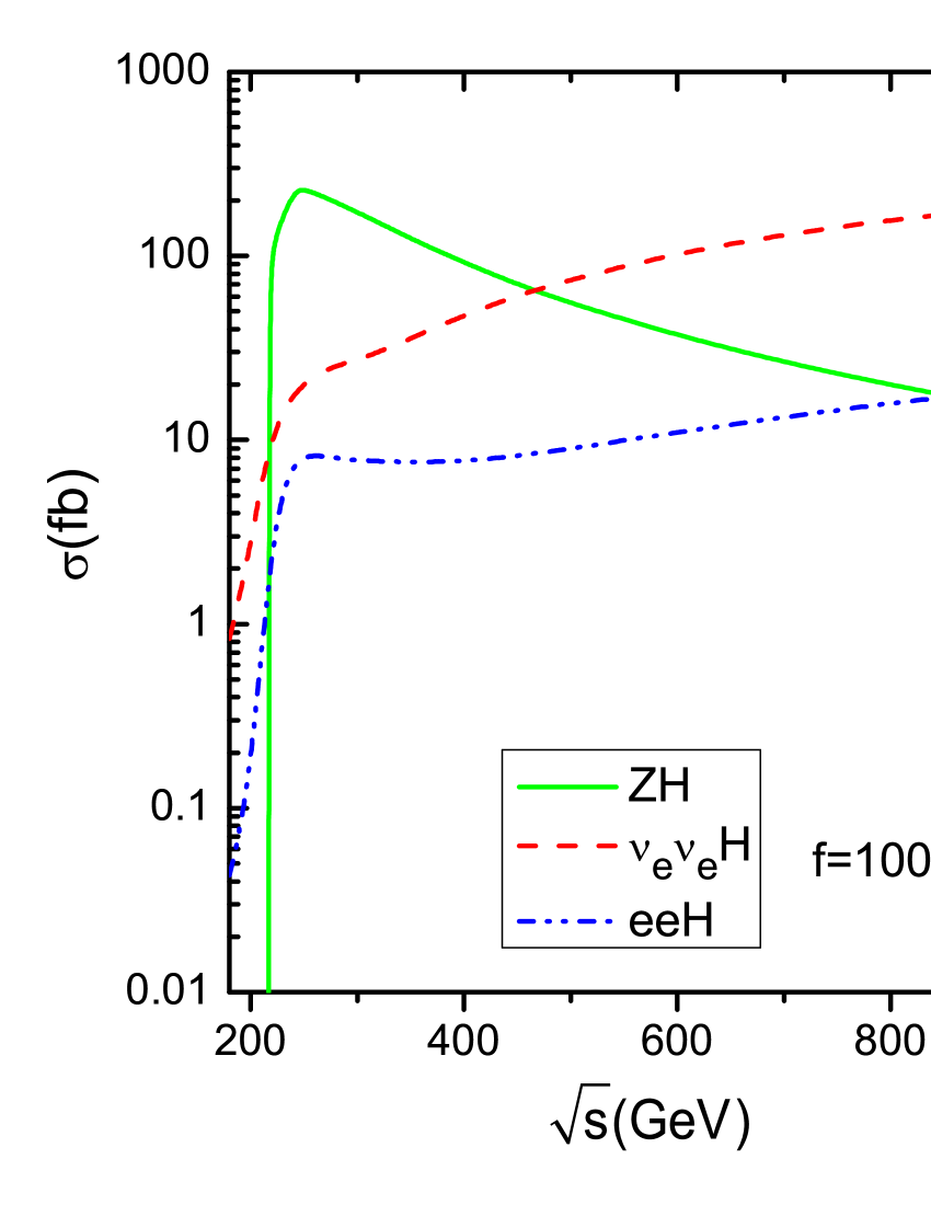
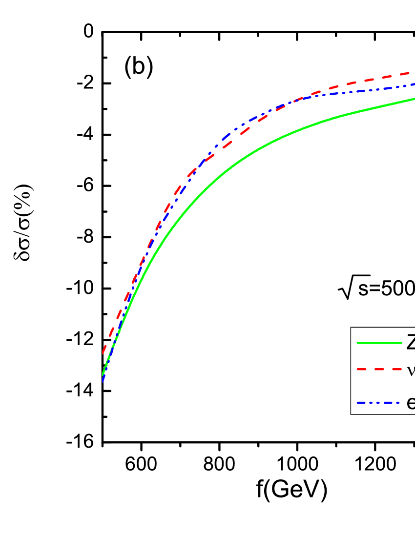
Figure 2: The production cross section $\sigma$ versus the center-of-mass energy $\sqrt{s}$ for $f=1000$ GeV(a) and the relative correction $\delta\sigma/\sigma$ versus the scale $f$ for $\sqrt{s}=500$ GeV(b) in the LHT model.

In Fig.2(a), we show the dependance of the production cross section $\sigma$ on the center-of-mass energy $\sqrt{s}$ for the scale $f=1000$ GeV in the LHT model. We present $ZH$, $\nu_{e}\bar{\nu}_{e}H$ and $e^{+}e^{-}H$ production channels, respectively. We can see that the $ZH$ production cross section dominates at low center-of-mass energies, the corresponding cross section increases sharply at the threshold and then decreases with the center-of-mass energy in proportion to $1/s$. The region of cross section maximum is around $240\sim 250$ GeV and the maximum value can reach about 230 fb. The $\nu_{e}\bar{\nu_{e}}H$ and $e^{+}e^{-}H$ production cross section increases with the center-of-mass energy in proportion to log$(s/m_{H}^{2})$ and hence becomes more important at energies $\sqrt{s}\geq 500$ GeV.

After the discovery of the Higgs-like boson at the LHC, in order to study the properties of this new particle with high precision, many schemes of the so-called Higgs factory have been proposed Higgsfactory . For example, the proposed LEP3 or China Higgs Factory (CHF) with a center-of-mass energy 240 GeV, the TLEP with a center-of-mass energy 350 GeV, the ILC with a center-of-mass energy 500 GeV, and so on. In Tab.I, we display the lowest-order dominant Higgs boson production cross section in the LHT model for different Higgs factories.

Table 1: Dominant Higgs-boson production cross section in the LHT model at various center-of-mass energies of the $e^{+}e^{-}$ collision for $f=1000$ GeV, $m_{H}=126$ GeV.

$\sqrt{s}$ [GeV]	$~{}~{}~{}240~{}~{}~{}$	$~{}~{}~{}350~{}~{}~{}$	$~{}~{}~{}500~{}~{}~{}$	$~{}~{}~{}1000~{}~{}~{}$
$\sigma(e^{+}e^{-}\rightarrow ZH)$[fb]	227	124	55.3	12.4
$\sigma(e^{+}e^{-}\rightarrow\nu_{e}\bar{\nu_{e}}H)$[fb]	21.1	35.7	74.6	203
$\sigma(e^{+}e^{-}\rightarrow e^{+}e^{-}H)$[fb]	7.9	7.5	8.9	20.4

In Fig.2(b), we show the dependance of the relative correction $\delta\sigma/\sigma$ on the scale $f$ for the center-of-mass energy $\sqrt{s}=500$ GeV. We present the relative correction $\delta\sigma/\sigma$ of $ZH$, $\nu_{e}\bar{\nu_{e}}H$ and $e^{+}e^{-}H$ production channels, respectively. We can see that the relative correction $\delta\sigma/\sigma$ decreases with the scale $f$ increasing, which means that the correction of the LHT model decouples with the scale $f$ increasing. For the three production channels, the relative corrections $\delta\sigma/\sigma$ are all negative and each of them can maximally reach $-13\%$ when the scale $f=500$ GeV. Moreover, we can see that the behaviors of the three production channels are similar due to the similar LHT correction to the $HZZ$ and $HWW$ couplings.

By combining the Higgs data from the LHC and electroweak precise measurements, the authors in Ref.LHTstatus get the constraint on the scale $f$ in the LHT model, that is, $f\geq 694$ GeV at $95\%$ CL. The direct searches for the new particles can also provide constraints on the scale $f$, but these bounds can be weaken by the small $k$. So, if we require the scale $f\geq 694$ GeV, the relative correction $\delta\sigma/\sigma$ of $ZH$ production can maximally reach $-7.5\%$ and the relative corrections $\delta\sigma/\sigma$ of $\nu_{e}\bar{\nu_{e}}H$ and $e^{+}e^{-}H$ production can both maximally reach $-6.5\%$.

By exploiting the $HZ\rightarrow Xl^{+}l^{-}$ channel, the $e^{+}e^{-}\rightarrow ZH$ production cross sections at $\sqrt{s}=350$ GeV with an integrated luminosity of 500 fb^-1 can be measured with statistical errors of $2.6\sim 3.1\%$ for Higgs-boson masses from 120 to 160 GeVzll . If the center-of-mass energy is upgraded to 500 GeV at a linear $e^{+}e^{-}$ collider, this will allow to measure the Higgs production cross sections at the level of a few percenthiggsMeasurement . So, the LHT effects can be tested at the future $e^{+}e^{-}$ colliders with a high luminosity.

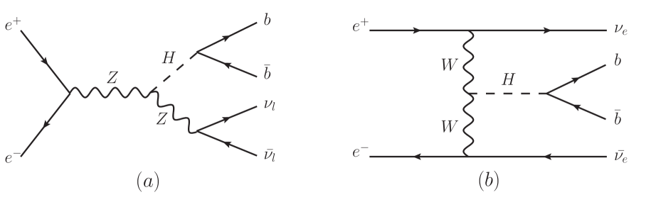
Figure 3: Feynman diagrams for $e^{+}e^{-}\rightarrow ZH$ followed by the subsequent $Z\rightarrow\nu_{l}\bar{\nu_{l}},H\rightarrow b\bar{b}$(a) and $e^{+}e^{-}\rightarrow\nu_{e}\bar{\nu_{e}}H$ followed by the subsequent $H\rightarrow b\bar{b}$(b).

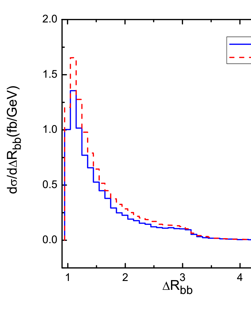
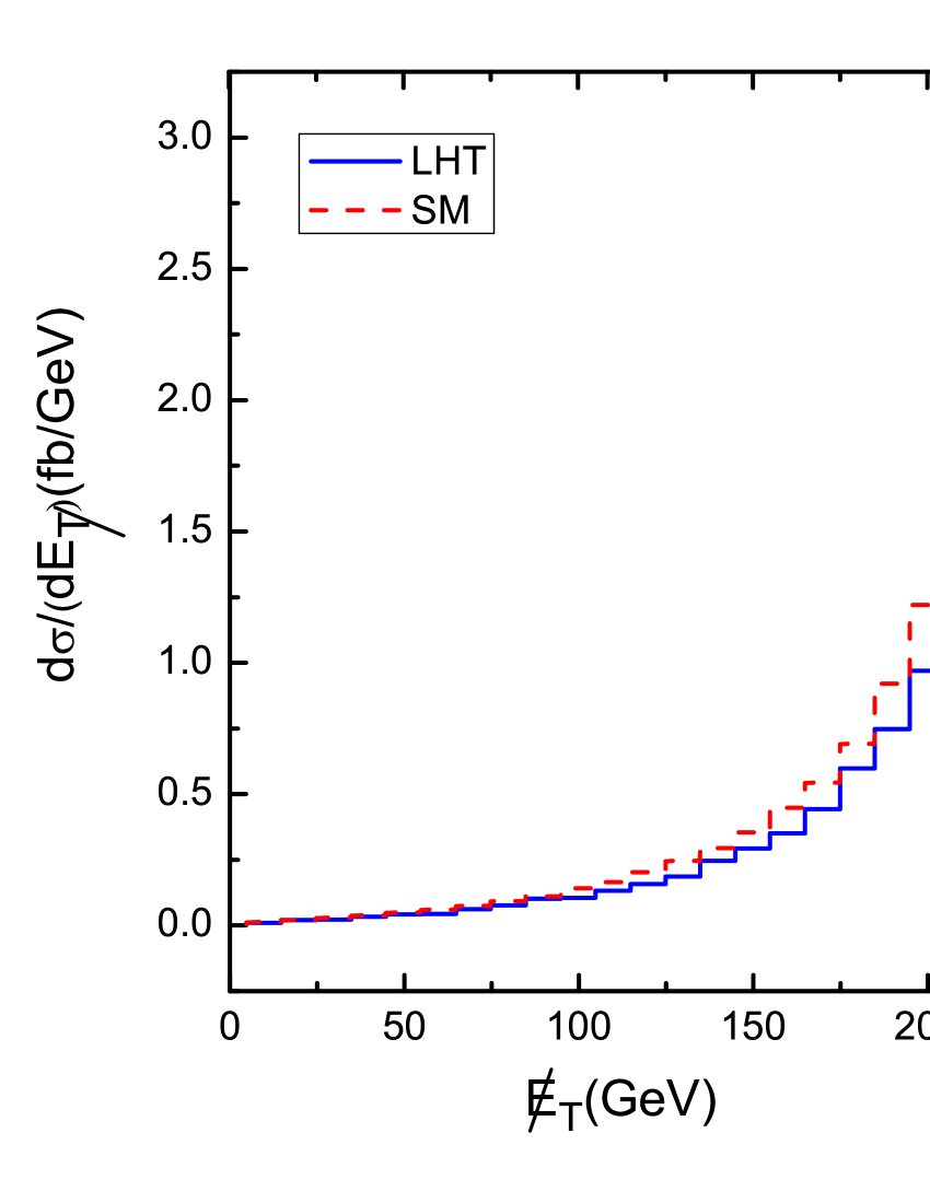
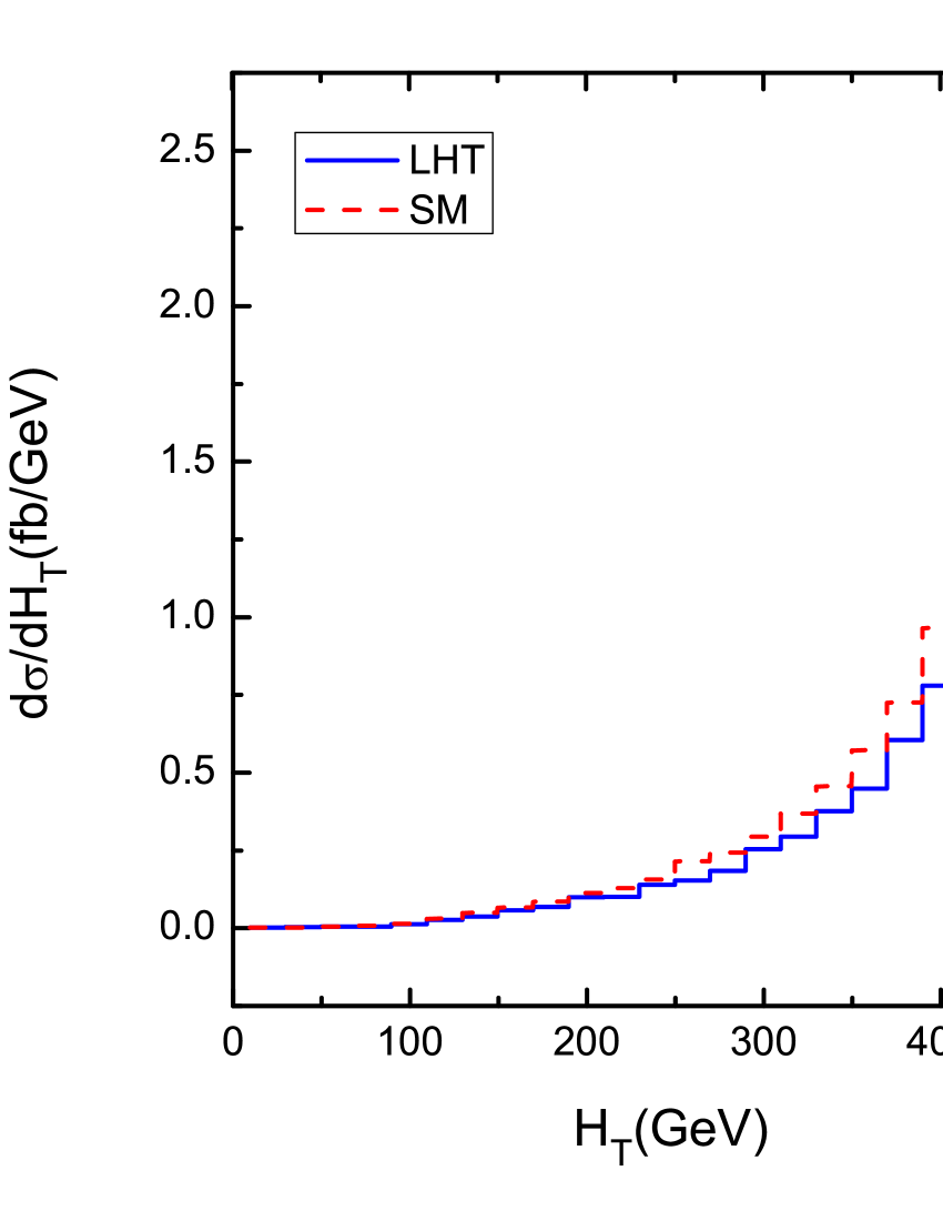
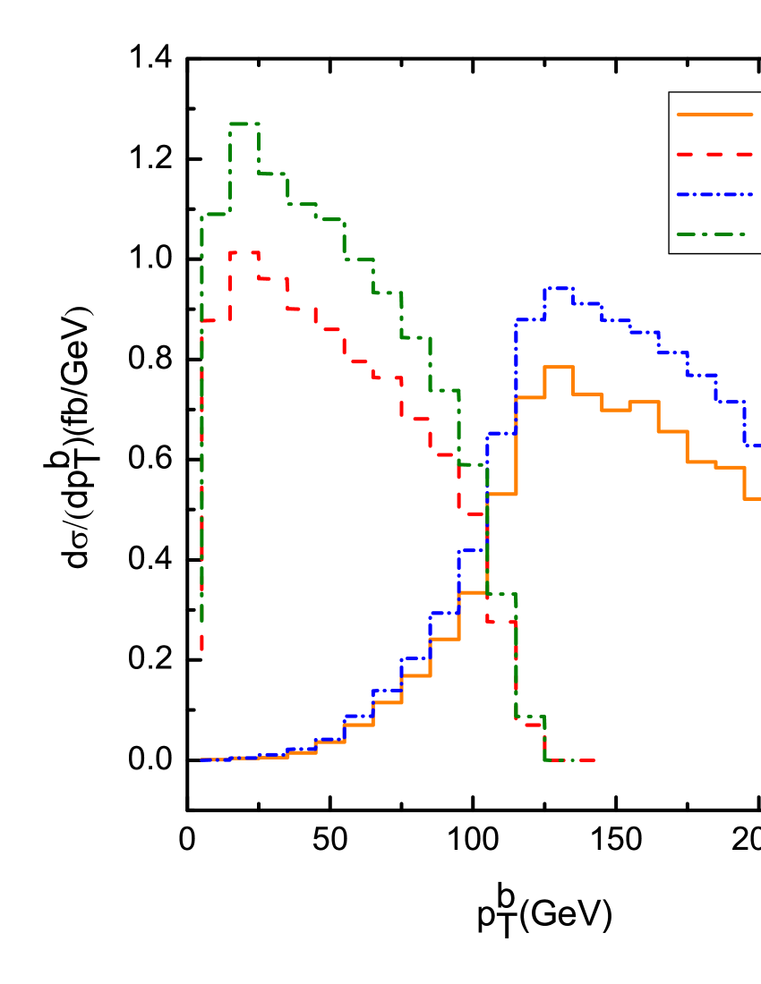
Figure 4: $\Delta R_{bb}$, $\not\!\!\!E_{T}$, $H_{T}$ and $p^{b}_{T}$ distributions of $e^{+}e^{-}\to ZH$ in the LHT and SM through the production of $e^{+}e^{-}\rightarrow ZH\rightarrow\nu_{l}\bar{\nu_{l}}b\bar{b}$ for $\sqrt{s}=500$ GeV, $f=700$ GeV.

In order to provide more information of the single Higgs-boson production, we display some kinematical distributions of final states by using Madgraph5mad5 . In Fig.4, we show the distributions of the production process $e^{+}e^{-}\rightarrow ZH$ for $\sqrt{s}=500$ GeV, $f=700$ GeV. We choose the $e^{+}e^{-}\rightarrow ZH\rightarrow\nu_{l}\bar{\nu_{l}}b\bar{b}$($l=e,\mu,\tau$) as the final states and the relevant Feynman diagram is shown in Fig.3(a). We display the separation between the two b-jets from Higgs boson ($\Delta R_{bb}\equiv\sqrt{(\Delta\phi)^{2}+(\Delta\eta)^{2}}$ ), the missing energy $\not\!\!\!E_{T}$, total transverse energy $H_{T}$ and the transverse momentum $p^{b}_{T}$ of di b-tagged jets in the LHT and the SM, respectively. We can see that the peak of the $\Delta R_{bb}$ is at $\Delta R_{bb}\sim 1$, the peak of the missing energy is at $\not\!\!\!E_{T}\sim 220$ GeV, and the peak of the total transverse energy is at $H_{T}\sim 440$ GeV. The transverse momentum $p^{b}_{T}$ for the two b-jets is different, one peak is at $p^{b1}_{T}\sim 130$ GeV and the other peak is at $p^{b2}_{T}\sim 20$ GeV.

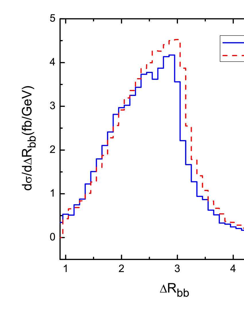
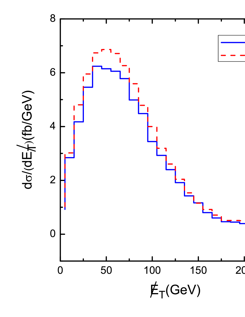
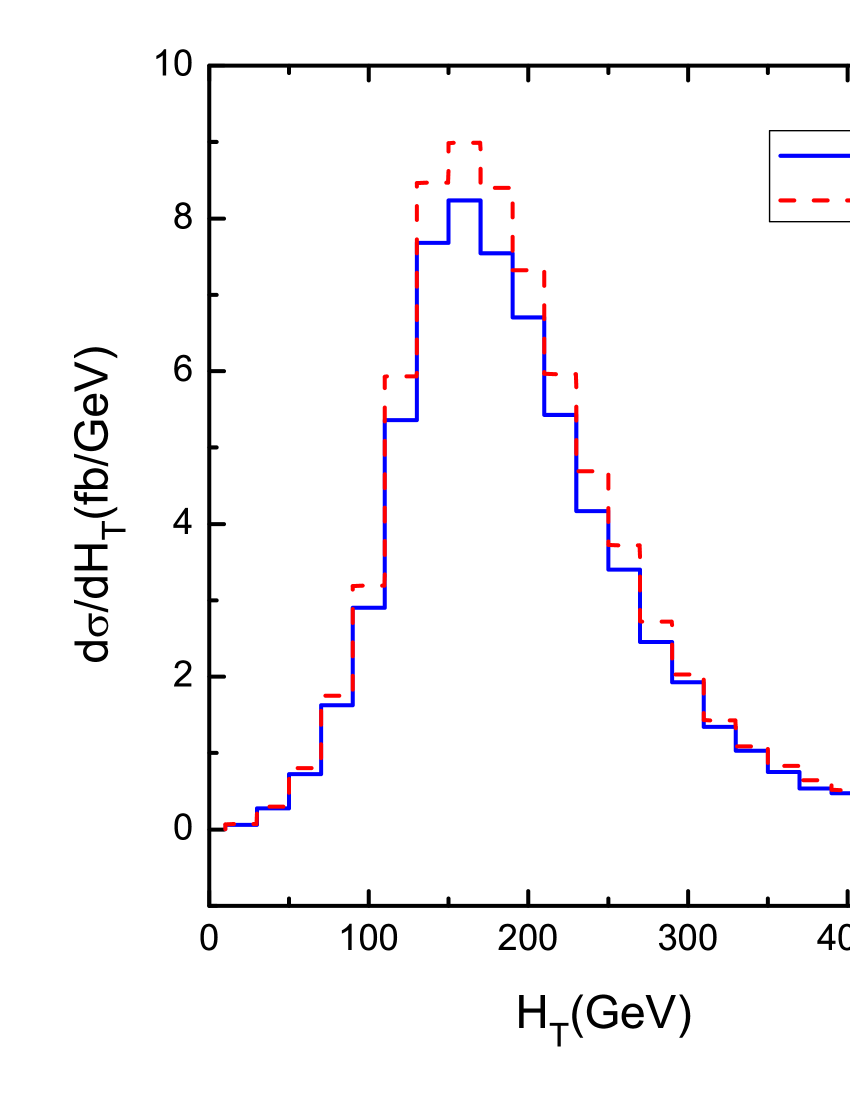
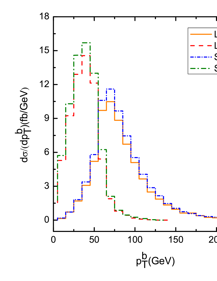
Figure 5: $\Delta R_{bb}$, $\not\!\!\!E_{T}$, $H_{T}$ and $p^{b}_{T}$ distributions of $e^{+}e^{-}\to\nu_{e}\bar{\nu_{e}}H$ in the LHT and SM through the production of $e^{+}e^{-}\rightarrow\nu_{e}\bar{\nu_{e}}H\rightarrow\nu_{e}\bar{\nu_{e}}b\bar{b}$ for $\sqrt{s}=500$ GeV, $f=700$ GeV.

In Fig.5, we show the distributions of production process $e^{+}e^{-}\to\nu_{e}\bar{\nu_{e}}H$ for $\sqrt{s}=500$ GeV, $f=700$ GeV. We choose the $e^{+}e^{-}\rightarrow\nu_{e}\bar{\nu_{e}}H\rightarrow\nu_{e}\bar{\nu_{e}}b\bar{b}$ as the final states and the relevant Feynman diagrams are shown in Fig.3(b). We display $\Delta R_{bb}$, $\not{E}_{T}$, $H_{T}$ and $p^{b}_{T}$ in the LHT and the SM, respectively. We can see that the peak of the $\Delta R_{bb}$ is at $\Delta R_{bb}\sim 3$, which means that the two b-jets incline to fly back-to-back. The peak of the missing energy is at $\not\!\!\!E_{T}\sim 50$ GeV, and the peak of the total transverse energy is at $H_{T}\sim 160$ GeV. The transverse momentum $p^{b}_{T}$ for the two b-jets is different, one peak is at $p^{b1}_{T}\sim 70$ GeV and the other peak is at $p^{b2}_{T}\sim 40$ GeV.

From Fig.4 and Fig.5, we can see that the behaviour of the relevant distributions in the LHT model is similar to that in the SM, and the LHT correction can obviously reduce the SM differential cross section at around the peak.

IV summary

In this paper, we studied the single Higgs-boson production at $e^{+}e^{-}$ colliders in the LHT model. The main production channels, such as $e^{+}e^{-}\rightarrow ZH$, $e^{+}e^{-}\rightarrow\nu_{e}\bar{\nu_{e}}H$ and $e^{+}e^{-}\rightarrow e^{+}e^{-}H$, have been taken into account. We calculated the production cross section and the relative correction at the tree level. Considering the latest constraints, we found that the relative correction of the $ZH$ production channel can reach $-7.5\%$ and the relative corrections of the $\nu_{e}\bar{\nu_{e}}H$ and $e^{+}e^{-}H$ production channels can both reach $-6.5\%$ for $\sqrt{s}=500$ GeV with the lower limit of the scale $f$(=694 GeV), which is large enough for people to detect the LHT effects at the future $e^{+}e^{-}$ colliders. In order to investigate the observability, some final state distributions of the production processes were presented.

References

- (1) S. Glashow, Nucl. Phys. 20 (1961) 579; A. Salam, in Elementary Particle Theory, ed. N. Svartholm, (1968); S. Weinberg, Phys. Rev. Lett. 19 (1967) 1264.
- (2) P. W. Higgs, Phys. Rev. Lett. 12 (1964) 132 and Phys. Rev. 145 (1966) 1156; F. Englert and R. Brout, Phys. Rev. Lett. 13 (1964) 321; G. S. Guralnik, C. R. Hagen and T. W. Kibble, Phys. Rev. Lett. 13 (1964) 585.
- (3) G. Aad et al. [ATLAS Collaboration], Phys. Lett. B 716 (2012) 1 [arXiv:1207.7214 [hep-ex]].
- (4) S. Chatrchyan et al. [CMS Collaboration], Phys. Lett. B 716 (2012) 30 [arXiv:1207.7235 [hep-ex]].
- (5) see examples: G. Belanger et al., arXiv:1210.1976; arXiv:1208.4952; J. F. Gunion, Y. Jiang, S. Kraml, Phys. Rev. D 86 (2012) 071702; Phys. Rev. Lett. 110 (2013) 051801; B. Yang, N. Liu and J. Han, arXiv:1308.4852 [hep-ph]; J. Cao, C. Han, L. Wu, J. M. Yang and Y. Zhang, JHEP 1211 (2012) 039, [arXiv:1206.3865 [hep-ph]]; C. Han, K. -i. Hikasa, L. Wu, J. M. Yang and Y. Zhang, JHEP 1310 (2013) 216, [arXiv:1308.5307 [hep-ph]]. J. Cao, L. Wu, P. Wu and J. M. Yang, JHEP 1309 (2013) 043, [arXiv:1301.4641 [hep-ph]]; C. Han, N. Liu, L. Wu, J. M. Yang and Y. Zhang, Eur. Phys. J. C 73 (2013) 2664, [arXiv:1212.6728].
- (6) E. Accomando et al. [ECFA/DESY LC Physics Working Group Collaboration], Phys. Rept. 299 (1998) 1, [hep-ph/9705442]; J. A. Aguilar-Saavedra et al., TESLA Technical Design Report Part III: Physics at an Linear Collider, [hep-ph/0106315]; K. Abe et al. [ACFA Linear Collider Working Group Collaboration], ACFA Linear Collider Working Group report, [hep-ph/0109166]; T. Abe et al. [American Linear Collider Working Group Collaboration], in Proc. of the APS/DPF/DPB Summer Study on the Future of Particle Physics (Snowmass 2001) ed. R. Davidson and C. Quigg, SLAC-R-570, Resource book for Snowmass 2001 [hep-ex/0106055, hep-ex/0106056, hep-ex/0106057, hep-ex/0106058]; Radoje Belusevic, KEK Preprint 2008-33, arXiv:0810.3187 [hep-ex]; S. Heinemeyer et al. [The Higgs Working Group at Snowmass ’05], CERN-PH-TH/2005-228, arXiv: hep-ph/0511332.
- (7) see examples: J. Fleischer and F. Jegerlehner, Nucl. Phys. B 216 (1983) 469; B. A. Kniehl, Z. Phys. C 55 (1992) 605; A. Denner, J. Küblbeck, R. Mertig and M. Böhm, Z. Phys. C 56 (1992) 261; F. A. Berends and R. Kleiss, Nucl. Phys. B 260 (1985) 32; Bernd A. Kniehl, Int.J.Mod.Phys. A17 (2002) 1457-1476; F. Jegerlehner and O. Tarasov, Nucl. Phys. Proc. Suppl. 116 (2003) 83 [hep-ph/0212004]; G. Belanger et al., Phys. Lett. B 559 (2003) 252 [hep-ph/0212261] and Nucl. Phys. Proc. Suppl. 116 (2003) 353 [hep-ph/0211268]; F. Boudjema et al., Phys. Lett. B600, 65(2004); Nucl. Instrum. Meth A 534 (2004) 334; A. Denner, S. Dittmaier, M. Roth and M. M. Weber, Phys. Lett. B 560 (2003) 196 [hep-ph/0301189]; Nucl. Phys. B 660 (2003) 289 [hep-ph/0302198]; Nucl. Phys. Proc. Suppl. 135 (2004)88-91.
- (8) see examples: H. Eberl, W. Majerotto and V. C. Spanos, Phys. Lett. B 538 (2002) 353 [hep-ph/ 0204280], Nucl. Phys. B 657 (2003) 378 [hep-ph/0210038], and hep-ph/0210330; T. Hahn, S. Heinemeyer and G. Weiglein, Nucl. Phys. B 652 (2003) 229 [hepph/ 0211204] and Nucl. Phys. Proc. Suppl. 116 (2003) 336 [hep-ph/0211384]; C. X. Yue, S. Z. Wang, and D. Q. Yu, Phys. Rev. D 68 (2003) 115004; C. X. Yue, W. Wang, Z. J. Zong, and F. Zhang, Eur. Phys. J C 42(2005) 331; Xuelei Wang, Yaobei Liu, Jihong Chen, Hua Yang, Eur. Phys. J. C 49 (2007) 593-597.
- (9) H. C. Cheng and I. Low, JHEP 0309 (2003) 051; JHEP 0408 (2004) 061; I. Low, JHEP 0410 (2004) 067; J. Hubisz and P. Meade, Phys. Rev. D 71 (2005) 035016.
- (10) Lei Wang, Wenyu Wang, Jin Min Yang, and Huajun Zhang,Phys. Rev. D 76 (2007) 017702; Lei Wang and Jin Min Yang,Phys. Rev. D 77 (2008) 015020; Phys. Rev. D 79 (2009) 055013.
- (11) A. Belyaev, C. -R. Chen, K. Tobe and C. -P. Yuan, Phys. Rev. D74 (2006) 115020. M. Blanke, A. J. Buras, A. Poschenrieder, S. Recksiegel, C Tarantino, S. Uhliga and A. Weilera, JHEP 01 (2007) 066; J. Hubisz, S. J. Leeb and G. Pazb, JHEP 06 (2006) 041; J. Hubisz and P. Meade, Phys. Rev. D71 (2005) 035016.
- (12) J.Beringer et al., (Particle Data Group), Phys. Rev. D 86 (2012) 010001.
- (13) J. Hubisz, P. Meade, A. Noble, and M. Perelstein, JHEP 0601 (2006) 135; Bingfang Yang, Xuelei Wang, and Jinzhong Han, Nucl. Phys. B 847 (2011) 1; J. Reuter, M. Tonini, JHEP 0213 (2013) 077; Xiao-Fang Han, Lei Wang, Jin Min Yang, Jingya Zhu, Phys. Rev. D 87 (2013) 055004; Jürgen Reuter, Marco Tonini, Maikel de Vries, arXiv:1307.5010 [hep-ph].
- (14) A. Blondel et al., arXiv:1302.3318 [physics.acc-ph].
- (15) Jürgen Reuter, Marco Tonini, Maikel de Vries, JHEP 1402 (2014) 053.
- (16) P. Garcia-Abia and W. Lohmann, EPJdirect C 2 (2000) 1; S. Heinemeyer et al., CERN-PH-TH/2005-228; hep-ph/0511332.
- (17) M. E. Peskin, arXiv:1207.2516 [hep-ph]; S. Dawson et al., arXiv:1310.8361[hep-ex]; D. M. Asner et al., arXiv:1310.0763 [hep-ph]; Howard Baer et al., The International Linear Collider Technical Design Report-Volume 2: Physics, arXiv:1306.6352 [hep-ph].
- (18) F. Maltoni and T. Stelzer, JHEP 0302 (2003) 027; J. Alwall et al., JHEP 0709 (2007) 028; J. Alwall et al., JHEP 1106 (2011) 128.