Abstract

The gamma density function is usually defined in interval between zero and infinity. This paper introduces an upper and a lower boundary to this distribution. The parameters which characterize the truncated gamma distribution are evaluated. A statistical test is performed on two samples of stars. A comparison with the lognormal and the four power law distribution is made.

Adv. Studies Theor. Phys, Vol. x, 200x, no. xx, xxx - xxx

A right and left truncated gamma

distribution with application to the stars

L. Zaninetti

Dipartimento di Fisica ,

Università degli Studi di Torino,

via P. Giuria 1, 10125 Torino, Italy

PACS: 97.10.-q; 97.20.-w;
Keywords: Stars: characteristics and properties of; Stars: normal;

1 Introduction

A probability distribution function (PDF) which models a given physical variable is usually defined in the interval $0\leq x<\infty$. As an example the exponential , the gamma, the lognormal, the Pareto and the Weibull PDFs are defined in such interval, see [1]. We now briefly review the status of the research on the truncated gamma distribution (TG). A first attempt to deduce the parameters of a TG can be found in [2], [3] derived the minimum variance unbiased estimate of the reliability function associated with the TG distribution which is right truncated, [4, 5] estimated the parameters of a TG distribution over $0\leq x<t$, adopting the maximum likelihood estimator(MLE), [6] studied the properties of TG distributions and derived the simulation algorithms which dominate the standard algorithms for these distributions, [7] considered a doubly-truncated gamma random variable restricted by both a lower (l) and upper (u) truncation.

On adopting an astronomical point of view the left truncation is connected with the minimum mass of a star, $\approx 0.02M_{\hbox{$\odot$}}$ and the right truncation with the maximum mass of a star, $\approx 60M_{\hbox{$\odot$}}$, see [8]. This paper first review the gamma PDF, introduces the right and left truncated gamma PDF and finally analyzes two samples of stars and brown dwarfs (BD).

2 The various gamma distributions

This Section reviews the gamma PDF, introduces the truncated gamma PDF and analyzes the data of two astronomical samples.

2.1 The gamma distribution

Let $X$ be a random variable taking values $x$ in the interval $[0,\infty]$; the gamma PDF is

$$f(x;b,c)=\frac{\left({\frac{x}{b}}\right)^{c-1}{{\rm e}^{-{\frac{x}{b}}}}}{b\Gamma\left(c\right)}$$ (1)

where

$$\mathop{\Gamma\/}\nolimits\!\left(z\right)=\int_{0}^{\infty}e^{{-t}}t^{{z-1}}dt\quad,$$ (2)

is the gamma function, $b>0$ is the scale and $c>0$ is the shape, see formula (17.23) in [5]. Its expected value is

$$E(x;b,c)=bc\quad,$$ (3)

and its variance,

$$Var(x;b,c)=b^{2}c\quad.$$ (4)

The mode is at

$$m(x;b,c)=bc-b\quad when\,c>1\,\quad.$$ (5)

The distribution function (DF) is

$$DF(x;b,c)=\frac{\gamma(c,\frac{x}{b})}{\Gamma\left(c\right)}\quad,$$ (6)

where

$$\mathop{\gamma\/}\nolimits\!\left(a,z\right)=\int_{0}^{z}t^{{a-1}}e^{{-t}}dt,$$ (7)

is the lower incomplete gamma function, see [9, 10]. The two parameters can be estimated by matching the moments

$$b=\frac{s^{2}}{\bar{x}}$$ (8)

$$c=(\frac{{\bar{x}}}{s})^{2}\quad,$$ (9)

where $s^{2}$ and $\bar{x}$ are the sample variance and the sample mean. More details can be found in [1].

2.2 The truncated gamma distribution

Let $X$ be a random variable taking values $x$ in the interval $[x_{l},x_{u}]$; the truncated gamma (TG) PDF is

$$f(x;b,c,x_{l},x_{u})=k\;\left({\frac{x}{b}}\right)^{c-1}{{\rm e}^{-{\frac{x}{b}}}}$$ (10)

where the constant $k$ is

$$k=\frac{c}{b\Gamma\left(1+c,{\frac{x_{{l}}}{b}}\right)-b\Gamma\left(1+c,{\frac{x_{{u}}}{b}}\right)+{{\rm e}^{-{\frac{x_{{u}}}{b}}}}{b}^{-c+1}{x_{{u}}}^{c}-{{\rm e}^{-{\frac{x_{{l}}}{b}}}}{b}^{-c+1}{x_{{l}}}^{c}}\quad,$$ (11)

where

$$\mathop{\Gamma\/}\nolimits\!\left(a,z\right)=\int_{z}^{\infty}t^{{a-1}}e^{{-t}}dt,$$ (12)

is the upper incomplete gamma function, see [9, 10]. Its expected value is

$$E(b,c,x_{l},x_{u})=-{b}^{2}k\left(-\Gamma\left(1+c,{\frac{x_{{l}}}{b}}\right)+\Gamma\left(1+c,{\frac{x_{{u}}}{b}}\right)\right)\quad.$$ (13)

The mode is at

$$m(x;b,c,x_{l},x_{u})=bc-b\quad when\,c>1\,\quad,$$ (14)

but in order to exist the inequality $x_{l}<m<x_{u}$ should be satisfied. The distribution function is

$$DF(x;b,c,x_{l},x_{u})=$$

$$k\left(b\Gamma\left(1+c,{\frac{x_{{l}}}{b}}\right)-b\Gamma\left(1+c,{\frac{x}{b}}\right)+{{\rm e}^{-{\frac{x}{b}}}}{b}^{-c+1}{x}^{c}-{{\rm e}^{-{\frac{x_{{l}}}{b}}}}{b}^{-c+1}{x_{{l}}}^{c}\right)\quad.$$ (15)

A random number generation can be implemented by solving for $x$ the following nonlinear equation

$$DF(x;b,c,x_{l},x_{u})-{\bf R}=0\quad,$$ (16)

where we have a pudendum number generator giving random numbers ${\bf R}$ between zero and one, see [11]. A simple derivation of the lower and upper boundaries gives

$$\tilde{x_{l}}=minimum~{}of~{}sample\quad\tilde{x_{u}}=maximum~{}of~{}sample\quad.$$ (17)

A first approximate derivation of $\tilde{b}$ and $\tilde{c}$ is through the standard estimation of parameters of the gamma distribution. We compute the $\chi^{2}$ with these first values of $\tilde{b}$ and $\tilde{c}$ and we search a numerical couple which gives the minimum $\chi^{2}$. The $\chi^{2}$ is computed according to the formula

$$\chi^{2}=\sum_{i=1}^{n}\frac{(T_{i}-O_{i})^{2}}{T_{i}},$$ (18)

where $n$ is the number of bins, $T_{i}$ is the theoretical value, and $O_{i}$ is the experimental value represented by the frequencies. The merit function $\chi_{red}^{2}$ is evaluated by

$$\chi_{red}^{2}=\chi^{2}/NF\quad,$$ (19)

where $NF=n-k$ is the number of degrees of freedom, $n$ is the number of bins, and $k$ is the number of parameters. The goodness of the fit can be expressed by the probability $Q$, see equation 15.2.12 in [12], which involves the degrees of freedom and the $\chi^{2}$. The Akaike information criterion (AIC), see [13], is defined by

$$AIC=2k-2ln(L)\quad,$$ (20)

where $L$ is the likelihood function and $k$ the number of free parameters in the model. We assume a Gaussian distribution for the errors and the likelihood function can be derived from the $\chi^{2}$ statistic $L\propto\exp(-\frac{\chi^{2}}{2})$ where $\chi^{2}$ has been computed by Equation (18), see [14], [15]. Now the AIC becomes

$$AIC=2k+\chi^{2}\quad.$$ (21)

2.3 Data analysis

A first test is performed on the low-mass initial mass function in the young cluster NGC 6611, see [16]. Table 1 shows the values of $\chi_{red}^{2}$, the AIC, the probability $Q$, of the astrophysical fits and the results of the K-S test, the maximum distance, $D$, between the theoretical and the astronomical DF as well the significance level $P_{KS}$ , see [17, 18, 19, 12]. Figure 1 shows the fit with the TG distribution of NGC 6611 and Figure 2 visually compares the three types of fits for NGC 6611.

Table 1: Numerical values of NGC 6611 cluster data (207 stars + BDs). The number of linear bins, $n$, is 20.

PDF	parameters	AIC	$\chi_{red}^{2}$	$Q$	D	$P_{KS}$
lognormal	$\sigma$=1.029,$\mu_{LN}=-1.258$	71.24	3.73	$1.3\,10^{-7}$	0.09366	0.04959
gamma	b=0.248 ,c = 1.717	62.83	3.26	3.15 $10^{6}$	0.109	0.0124
truncated  gamma	b=0.372 ,c =1.287	52.34	2.77	0.00017	0.09	0.061
	$x_{l}$=0.019, $x_{u}$=1.46
four	Eqn.(59)	81.39	5.18	$2.41\,19^{-9}$	0.12514	$2.72\,10^{-3}$
power  laws	in Zaninetti 2013

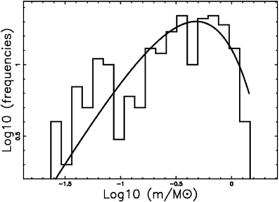
Figure 1: Logarithmic histogram of mass distribution as given by NGC 6611 cluster data (207 stars + BDs) with a superposition of the TG distribution when the number of bins, $n$, is 12, $c$ = 1.287 , $b$ = 0.372 , $x_{l}$ = 0.019 and $x_{u}$ =1.36. Vertical and horizontal axes have logarithmic scales.

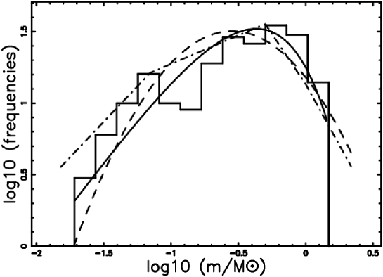
Figure 2: Histogram (step-diagram) of mass distribution as given by NGC 6611 cluster data (207 stars + BDs) with a superposition of the left TG distribution (full line), the lognormal (dashed), and the four power laws (dot-dash-dot-dash). Vertical and horizontal axes have logarithmic scales.

A second test is performed on low-mass stars in NGC 2362, see [20]. Table 2 shows the statistical parameters which characterize the astrophysical fits. Figure 3 shows the fit with the TG distribution of NGC 2362 and Figure 4 visually compares the three types of fits for NGC 2362.

Table 2: Numerical values of of the NGC 2362 cluster data (272 stars). The number of linear bins, $n$, is 20.

PDF	parameters	AIC	$\chi_{red}^{2}$	$Q$	D	$P_{KS}$
lognormal	$\sigma$=0.5,$\mu_{LN}=-0.55$	37.64	1.86	0.013	0.07305	0.10486
gamma	b=0.13 ,c =4.955	34.28	1.68	0.034	0.059	0.284
truncated  gamma	b=0.161 ,c =3.933	33.88	1.61	0.055	0.071	0.122
	$x_{l}$=0.12, $x_{u}$=1.47
four	Eqn.(58)	77.608	4.89	$1.17\,10^{-8}$	0.16941	$2.6\,10^{-7}$
power  laws	in Zaninetti 2013

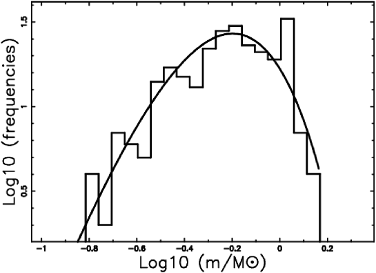
Figure 3: Logarithmic histogram of mass distribution as given by NGC 2362 cluster data (272 stars) with a superposition of the TG distribution when the number of bins, $n$, is 12, $b=0.161$, $c=3.933$, $x_{l}$= 0.12 and $x_{u}$ =1.47 . Vertical and horizontal axes have logarithmic scales.

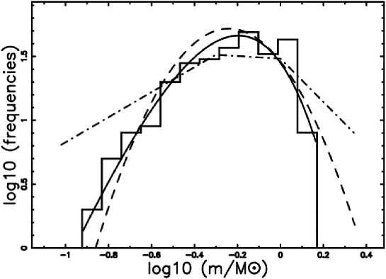
Figure 4: Histogram (step-diagram) of mass distribution as given by NGC 2362 cluster data (272 stars) with a superposition of the left TG distribution (full line), the lognornal (dashed), and the four power laws (dot-dash-dot-dash). Vertical and horizontal axes have logarithmic scales.

3 Conclusions

The right or left TG PDF has been extensively investigated in the field of mathematics , as an example [7] reports most of the mathematical details. The application of the TG PDF in astronomy represents conversely a new promising field. Here we have deduced the constant of normalization ,eqn.(11), the average value ,eqn.(13), the DF , eqn.(15), and presented an algorithm for the generation of the random numbers , (eqn.16). The application of the TG PDF to the IMF is positive and both the reduced $\chi^{2}$ and the K-S test give better results in respect to the standard PDFs used by the astronomers which are the lognormal and the four power laws , see Tables 1 and 2. A comparison with the left truncated beta PDF , see Tables 1 and 2 in [21] allows to say that the left truncated beta PDF produces a better fit to the IMF in respect to the truncated gamma PDF here analyzed.

References

- [1] M. Evans, N. Hastings, B. Peacock, Statistical Distributions - third edition, John Wiley & Sons Inc, New York, 2000.
- [2] D. G. Chapman, Estimating the parameters of a truncated gamma distribution, The Annals of Mathematical Statistics 27 (2) (1956), 498–506.
- [3] G. Baikunth Nath, Unbiased estimates of reliability for the truncated gamma distribution, Scandinavian Actuarial Journal 1975 (3) (1975), 181–186.
- [4] L. M. Hegde, R. C. Dahiya, Estimation of the parameters of a truncated gamma distribution, Communications in Statistics - Theory and Methods 18 (2) (1989), 561–577.
- [5] N. L. Johnson, S. Kotz, N. Balakrishnan, Continuous univariate distributions. Vol. 1. 2nd ed., Wiley , New York, 1994.
- [6] A. Philippe, Simulation of right and left truncated gamma distributions by mixtures, Statistics and Computing 7 (3) (1997), 173–181.
- [7] C. S. Coffey, K. E. Muller, Properties of doubly-truncated gamma variables, Communications in Statistics - Theory and Methods 29 (4) (2000), 851–857.
- [8] P. Kroupa, C. Weidner, J. Pflamm-Altenburg, I. Thies, J. Dabringhausen, M. Marks, T. Maschberger, The Stellar and Sub-Stellar Initial Mass Function of Simple and Composite Populations, 2013, 115.
- [9] M. Abramowitz, I. A. Stegun, Handbook of mathematical functions with formulas, graphs, and mathematical tables, Dover, New York, 1965.
- [10] F. W. J. e. Olver, D. W. e. Lozier, R. F. e. Boisvert, C. W. e. Clark, NIST handbook of mathematical functions., Cambridge University Press. , Cambridge, 2010.
- [11] D. Kahaner, C. Moler, S. Nash, Numerical Methods and Software, Prentice Hall Publishers, Englewood Cliffs, New Jersey, 1989.
- [12] W. H. Press, S. A. Teukolsky, W. T. Vetterling, B. P. Flannery, Numerical Recipes in FORTRAN. The Art of Scientific Computing, Cambridge University Press, Cambridge, 1992.
- [13] H. Akaike, A new look at the statistical model identification, IEEE Transactions on Automatic Control 19 (1974), 716–723.
- [14] A. R. Liddle, How many cosmological parameters?, MNRAS 351 (2004), L49–L53.
- [15] W. Godlowski, M. Szydowski, Constraints on Dark Energy Models from Supernovae, in: M. Turatto, S. Benetti, L. Zampieri, W. Shea (Eds.), 1604-2004: Supernovae as Cosmological Lighthouses, Vol. 342 of Astronomical Society of the Pacific Conference Series, 2005, 508–516.
- [16] J. M. Oliveira, R. D. Jeffries, J. T. van Loon, The low-mass initial mass function in the young cluster NGC 6611 , MNRAS 392 (2009), 1034–1050.
- [17] A. Kolmogoroff, Confidence limits for an unknown distribution function, The Annals of Mathematical Statistics 12 (4) (1941), 461–463.
- [18] N. Smirnov, Table for estimating the goodness of fit of empirical distributions, The Annals of Mathematical Statistics 19 (2) (1948), 279–281.
- [19] J. Massey, Frank J., The kolmogorov-smirnov test for goodness of fit, Journal of the American Statistical Association 46 (253) (1951), 68–78.
- [20] J. Irwin, S. Hodgkin, S. Aigrain, J. Bouvier, L. Hebb, M. Irwin, E. Moraux, The Monitor project: rotation of low-mass stars in NGC 2362 - testing the disc regulation paradigm at 5 Myr, MNRAS 384 (2008), 675–686.
- [21] L. Zaninetti, The initial mass function modeled by a left truncated beta distribution , ApJ 765 (2013), 128–135.