Anisotropic merging and splitting of dipolar Bose-Einstein condensates

Abstract

We study the merging and splitting of quasi-two-dimensional Bose-Einstein condensates with strong dipolar interactions. We observe that if the dipoles have a non-zero component in the plane of the condensate, the dynamics of merging or splitting along two orthogonal directions, parallel and perpendicular to the projection of dipoles on the plane of the condensate are different. The anisotropic merging and splitting of the condensate is a manifestation of the anisotropy of the roton-like mode in the dipolar system. The difference in dynamics disappears if the dipoles are oriented at right angles to the plane of the condensate as in this case the Bogoliubov dispersion, despite having roton-like features, is isotropic.

I Introduction

The first experimental generation of a Bose-Einstein condensate (BEC) in a gas of chromium (⁵²Cr) atoms Griesmaier ; Lahaye-1 ; Koch , which have permanent magnetic dipole moments, has lead to a flurry of experimental and theoretical investigations on dipolar quantum gases. These have been reviewed in Refs. Lahaye-2 ; Baranov . Besides ⁵²Cr, dipolar Bose-Einstein condensates (DBECs) of dysprosium (¹⁶⁴Dy) Lu-1 and erbium (¹⁶⁸Eb) Aikawa have also been experimentally realized. Quantum degeneracy has also been realized in dipolar Fermi gases of dysprosium (¹⁶¹Dy) Lu-2 and erbium (¹⁶⁷Eb) K_Aikawa . The two important characteristics of the dipolar interaction are its long range and anisotropic nature. The anisotropy introduced by the dipolar interactions has been observed in the the expansion dynamics Stuhler and the collective excitations of a ⁵²Cr condensate Bismut-2 . In contrast to contact interactions, all partial waves contribute to the scattering amplitude in the case of dipolar interactions. This makes the inter-particle interactions momentum dependent Lahaye-2 . As a consequence, the DBECs can support roton like excitations Santos ; Wilson-1 ; Wilson-2 . The presence of a roton like mode in spectrum of the dipolar Bose-Einstein condensate (DBEC) lowers the Landau critical speed Landau below the speed of sound for sufficiently large particle numberWilson-2 . Roton excitations can lead to density fluctuations at defects like vortices Wilson-1 ; Yi and a roton instability Santos ; Ronen ; Wilson-3 . It has been demonstrated theoretically that the static and dynamic structure factors which can be measured using Bragg spectroscopy Blakie , atom-number fluctuations in a trapped DBEC Bisset , and the response of the condensate to weak lattice potentials Corson-1 ; Corson-2 ; Jona-Lasinio-1 can reveal the presence of the, still experimentally elusive, roton excitations. Roton excitations also enhance the density fluctuations in two-dimensional DBECs Boudjemaa . The density dependence of the roton minimum also results in the spatial confinement of the rotons in trapped DBECs Jona-Lasinio-2 . In addition to these, dipolar interactions lead to anisotropic superfluidity, which, strictly speaking, is just the anisotropic manifestation of a roton like mode in the dipolar system Fischer ; Ticknor ; Muruganandam . The anisotropic excitation spectrum of the dipolar condensate of ⁵²Cr has also been measured experimentally Bismut-1 . In the present work, we study the dynamics of the merging and splitting of the DBEC of ⁵²Cr with a partially tilted polarization into the plane of the motion using a non-local Gross-Pitaevskii equation. The anisotropic coherence properties of such a DBEC at finite temperatures have been studied using Hartree-Fock-Bogoliubov method within the Popov approximation (HFBP) Ticknor-2 . We find that the anisotropic superfluidity of these systems manifests itself as the directional dependence of the merging and splitting dynamics.

The non-adiabatic merging and splitting of Bose-Einstein condensates (BECs) with pure contact interactions is known to lead to the formation of dispersive shock waves Chang . In the context of shock waves, the decay of small density defects into quantum shock waves was earlier observed in BECs Dutton . The non-adiabatic collision of two strongly interacting Fermi gases leading to the formation of shock waves has also been studied Joseph ; Bulgac ; Ancilotto . The propagation and nonlinear response of dispersive shock waves, including the interaction of colliding shock waves, in one and two-dimensional non-linear Kerr like media have also been investigated Wan . The interatomic interactions in these various studies were isotropic. This is no longer the case for DBECs, which are the focus of our study in the present work.

The paper is organized as follows- We start by providing the mean-field description of DBECs in Sec. II. Here we discuss the quasi-two-dimensional non-local Gross-Pitaevskii equation (GPE) which we employ to study the DBEC with an arbitrary direction of polarization. In Sec. III, after analyzing the validity of the quasi-two-dimensional GPE, we numerically investigate the splitting and merging dynamics of DBEC. We finally conclude by providing a summary of results in Sec. IV.

II Mean Field Description of Dipolar Bose-Einstein condensate

In the mean field regime, a scalar DBEC at $T=0$ K can be well described by the non-local GPE Lahaye-2 ; Baranov

$$i\hbar\frac{\partial\Phi(\mathbf{x},t)}{\partial t} = \left[-\frac{\hbar^{2}\nabla^{2}}{2m}+V(\mathbf{x})+g|\Phi(\mathbf{x},t)|^{2}\right.$$

$$\left.+\int U_{\rm dd}(\mathbf{x-x^{\prime}})|\Phi(\mathbf{x}^{\prime},t)|^{2}d\mathbf{x}^{\prime}\right]\Phi(\mathbf{x},t),$$

where $\Phi(\mathbf{x},t)$ is the wave function of the condensate. The non-local term, the last term in the parenthesis, accounts for the long range dipole-dipole interaction. In case the dipolar gas is polarized, i.e., all the dipoles are oriented along the same direction, the dipole-dipole interaction energy is

$$U_{\rm dd}=\frac{C_{\rm dd}}{4\pi}\frac{1-3\cos^{2}\theta}{|\mathbf{x}-\mathbf{x}^{\prime}|^{3}},$$ (2)

where $\theta$ is the angle between the direction of polarization and relative position vector of the dipoles. The coupling constant $C_{\rm dd}=12\pi\hbar^{2}a_{\rm dd}/m$, where $a_{\rm dd}$ is the length characterizing the strength of the dipolar interactions and $m$ is the mass of the atom. For the dipolar gas consisting of atoms with permanent magnetic dipole moment $\chi$ like ⁵²Cr, $a_{\rm dd}=\mu_{0}\chi^{2}m/(12\pi\hbar^{2})$, where $\mu_{0}$ is the permeability of the free space. The harmonic trapping potential $V(\mathbf{x})=m(\omega_{x}^{2}x^{2}+\omega_{y}^{2}y^{2}+\omega_{z}^{2}z^{2})/2$, where $\omega_{j}$’s with $j=x,y,z$ are trapping frequencies along the three coordinate axes. The contact interaction between atoms is characterized by the interaction strength $g=4\pi\hbar^{2}a/m$, where $a$ is the $s$-wave scattering length. The total number of atoms $N$ and energy $E$ are conserved by Eq. (II). For the sake of solving Eq. (II) numerically, we transform the GP equation into dimensionless form using following transformations:

$$\mathbf{x} = \tilde{\mathbf{x}}a_{\rm osc},~{}t=2\tilde{t}\omega^{-1},~{}\Phi=\sqrt{N}\tilde{\Phi}a_{\rm osc}^{-3/2},$$ (3)

where $a_{\rm osc}=\sqrt{\hbar/(m\omega)}$ with $\omega=\rm min~{}\{\omega_{x},\omega_{y},\omega_{z}\}$ is the oscillator length. The dimensionless GP equation for the DBEC is now of the form

$$i\frac{\partial\tilde{\Phi}}{\partial\tilde{t}} = \left[-\tilde{\nabla}^{2}+2\tilde{V}+2\tilde{g}|\tilde{\Phi}|^{2}+\right.$$ (4)

$$\left.2\int U_{\rm dd}(\tilde{\mathbf{x}}-\tilde{\mathbf{x^{\prime}}})|\tilde{\Phi}(\tilde{\mathbf{x^{\prime}}})|^{2}d\tilde{\mathbf{x^{\prime}}}\right]\tilde{\Phi},$$

where $\tilde{V}=(\lambda_{x}^{2}\tilde{x}^{2}+\lambda_{y}^{2}\tilde{y}^{2}+\lambda_{z}^{2}\tilde{z}^{2})/2$, $\lambda_{j}=\omega_{j}/\omega$ with $j=x,y,z$ and $\tilde{g}=4\pi\hbar aN/(m\omega a_{\rm osc}^{3})$. In order to simplify the notations, from here on we will write these variables without tildes unless mentioned otherwise. In the present work, we consider the DBEC in a quasi-two-dimensional trap for which $\lambda_{x}=\lambda_{y}=1\ll\lambda_{z}$. In this case, the axial degrees of freedom of the system are frozen, and the chemical potential in scaled units $\mu_{3d}<\lambda_{z}$ Gorlitz . Here the chemical potential $\mu_{3d}$ in scaled units is defined as

$$\mu_{3d} = \int\left[\frac{|\nabla\Phi(\mathbf{x})|^{2}}{2}+V(\mathbf{x})|\Phi(\mathbf{x})|^{2}+g|\Phi(\mathbf{x})|^{4}+\right.$$ (5)

$$\left.\Phi^{*}(\mathbf{x})\int U_{\rm dd}(\mathbf{x}-\mathbf{x^{\prime}})|\Phi(\mathbf{x^{\prime}})|^{2}d\mathbf{x^{\prime}}\right]\Phi(\mathbf{x})d\mathbf{x}.$$

We write $\Phi(\mathbf{x})=\zeta(z)\phi(x,y)$ with $\zeta(z)=(\lambda_{z}/\pi)^{1/4}e^{-(\lambda_{z}z^{2})/2}$ as the harmonic oscillator ground state along the axial direction. After integrating out the axial coordinate, we obtain the following two-dimensional equation Pedri ; Muruganandam-1 ; Fischer ; Ticknor :

$$i\frac{\partial\phi}{\partial t} = \left\{-\nabla_{\rho}^{2}+2V_{\rho}+2g_{\rho}|\phi|^{2}+4\sqrt{2\pi\lambda_{z}}a_{\rm dd}N\right.$$ (6)

$$\times\int\frac{d^{2}k_{\rho}}{4\pi^{2}}e^{i\mathbf{k}_{\rho}.\tilde{\rho}}\tilde{n}(\mathbf{k}_{\rho})\left[\cos^{2}(\alpha)h_{2d}^{\perp}\left(\frac{\mathbf{k}_{\rho}}{\sqrt{2\lambda_{z}}}\right)\right.$$

$$\left.\left.+\sin^{2}(\alpha)h_{2d}^{\parallel}\left(\frac{\mathbf{k}_{\rho}}{\sqrt{2\lambda_{z}}}\right)\right]\right\}\phi,$$

where $\nabla_{\rho}^{2}=\partial^{2}/\partial x^{2}+\partial^{2}/\partial y^{2}$, $V_{\rho}=x^{2}/2+y^{2}/2$ and $g_{\rho}=\sqrt{\lambda_{z}/2\pi}g$. It must be pointed out here that the term $\lambda_{z}\phi$, arising from the axial energy, has been neglected from the right hand side of the Eq. (6) as it only decreases the chemical potential and energy by an amount of $\lambda_{z}\hbar\omega/2$ without affecting the dynamics Salasnich . Here we have considered an arbitrary direction of polarization in the $xz$ plane, which makes an angle $\alpha$ with the $z$ axis, and $h_{2d}^{\perp}(\mathbf{k}_{\rho}/\sqrt{2\lambda_{z}})$ and $h_{2d}^{\parallel}(\mathbf{k}_{\rho}/\sqrt{2\lambda_{z}})$ are defined as

$$h_{2d}^{\perp}\left(\frac{\mathbf{k}_{\rho}}{\sqrt{2\lambda_{z}}}\right) = 2-\frac{3\sqrt{\pi}k_{\rho}}{\sqrt{2\lambda_{z}}}\exp\left(\frac{k_{\rho}^{2}}{2\lambda_{z}}\right){\rm erfc}\left(\frac{k_{\rho}}{\sqrt{2\lambda_{z}}}\right),$$

$$h_{2d}^{\parallel}\left(\frac{\mathbf{k}_{\rho}}{\sqrt{2\lambda_{z}}}\right) = -1+\frac{3\sqrt{\pi}k_{x}^{2}}{\sqrt{2\lambda_{z}}k_{\rho}}\exp\left(\frac{k_{\rho}^{2}}{2\lambda_{z}}\right){\rm erfc}\left(\frac{k_{\rho}}{\sqrt{2\lambda_{z}}}\right).$$

The scaled wavefunction is normalized to unity, i.e., $\int|\phi|^{2}d\rho=1$. We use the time splitting Fourier spectral method to solve equation Eq. (6) Bao . The spatial and time step sizes employed in the present work are $0.1~{}a_{\rm osc}$ and $0.0005~{}{\omega^{-1}}$ respectively.

III Merging and splitting dynamics of the DBEC

In the present work, we consider $5\times 10^{4}$ (or $10^{5}$) atoms of ⁵²Cr in a trapping potential with $\omega_{x}=\omega_{y}=\omega=2\pi\times 10$ Hz and $\omega_{z}=2\pi\times 980$ Hz. Hence, the units of length and time employed are $a_{\rm osc}=4.4~{}\mu$m and $\omega^{-1}=1.59\times 10^{-2}$s respectively. The dipolar length of ⁵²Cr is $16~{}a_{0}$ and the background $s$-wave scattering length is $100~{}a_{0}$ Lahaye-1 . The $s$-wave scattering length of ⁵²Cr can be tuned by magnetic Feshbach resonances Lahaye-1 ; Werner . However, we consider $a=8~{}a_{0}$, which is significantly smaller than its background value, in order to accentuate the effects of dipolar interactions.

Before proceeding further, let us first analyze the validity of the Eq. (6) used in the present work. To this end, we solve the full three dimensional GP equation (II) with $N=5\times 10^{4}$ and $N=10^{5}$ atoms of the ⁵²Cr for the aforementioned trapping potential parameters with $a=8~{}a_{0}$, $a_{\rm dd}=16a_{0}$, and with dipoles oriented along $z$-axis ($\alpha=0$). We use imaginary time propagation method, where $t$ is replaced by $-i\tau$, to obtain the ground state solution of Eq. (II). The spatial and temporal (imaginary time) step sizes used to solve Eq. (II) are $\delta x=\delta y=0.1$, $\delta z=0.02$, and $\delta\tau=0.0005$ respectively. By integrating out the $x$ and $y$ dependence of the total density $|\Phi(x,y,z)|^{2}$, we calculate the one-dimensional density along $z$-axis, i.e.,

$$|\Phi_{1d}(z)|^{2}=\int|\Phi(x,y,z)|^{2}dxdy.$$ (7)

In Fig. 1, we have shown the variation of this one-dimensional density $|\Phi_{1d}(z)|^{2}$ corresponding to the ground state solution and $|\zeta(z)|^{2}$ with respect to axial coordinate. As is evident from the Figs. 1(a) and (b), the one-dimensional density along the axial direction is very close to the density corresponding to the harmonic oscillator ground state along the same direction. This justifies the splitting of total wavefunction as $\Phi(x,y,z)=\phi(x,y)\zeta(z)$, and therefore the use of Eq. (6) in the present work. Moreover, the chemical potential values obtained by solving the full three-dimensional GP Eq. (II) and then using Eq. (5) are $\mu_{3d}=66.0~{}\hbar\omega$ and $\mu_{3d}=73.1~{}\hbar\omega$ for $N=5\times 10^{4}$ and $N=10^{5}$ respectively. Hence, $\mu_{3d}<\hbar\omega_{z}=98~{}\hbar\omega$ in both the cases as is necessary for the system to be in quasi-two-dimensional regime Gorlitz . Here, it is pertinent to point out that by replacing $\zeta(z)$ with an ansatz which is the superposition of zeroth and second harmonic oscillator wave functions with variable width and relative amplitude, a more accurate two-dimensional GP equation has been suggested by Wilson et al. Wilson-4 . It has also been shown in the context of quasi-two-dimensional bright solitons in the dipolar condensates that the non-linear coupling can lead to the deposition of the excitation energy along the tightly bound direction Eichler . However, very strong confinement along axial direction in the present work ensures that the frozen Gaussian approximation along this direction is a reasonably good approximation.

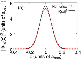
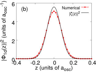
Figure 1: Variation of $|\Phi_{1d}(z)|^{2}$ corresponding to the ground state solution and $|\zeta(z)|^{2}$ as a function of $z$ for (a) $N=5\times 10^{4}$ and (b) $N=10^{5}$. The black and red curves correspond to $|\zeta(z)|^{2}$ and $|\Phi_{1d}(z)|^{2}$ respectively.

III.1 Merging of two DBEC fragments

In order to divide the DBEC into two fragments, we apply a Gaussian obstacle potential, in addition to the harmonic trapping potential mentioned earlier, on the condensate. Now, to study the effect of anisotropic superfluidity, introduced by a non-zero component of the dipoles in the $xy$ plane, on the merging dynamics, we consider the following two obstacle potentials

$$V^{\perp}_{\rm obs} = V_{0}\exp\left(-2\frac{x^{2}}{w_{0}^{2}}\right),$$ (8)

$$V^{\parallel}_{\rm obs} = V_{0}\exp\left(-2\frac{y^{2}}{w_{0}^{2}}\right),$$ (9)

here $V_{0}=100~{}\hbar\omega$ is the amplitude of the Gaussian potential and $w_{0}=2.5~{}\mu$m is its width. Applying $V^{\perp}_{\rm obs}$ creates a repulsive barrier potential along $y$-axis, i.e., perpendicular to the tilt of the dipoles on $xy$-plane, whereas applying $V^{\parallel}_{\rm obs}$ creates a repulsive barrier potential along the $x$-axis, i.e., parallel to the tilt of the dipoles. We now consider two cases in order to contrast the anisotropic merging dynamics with the isotropic one.

Anisotropic merging: Here we take the angle $\alpha$ to be $\pi/4$. We first obtain the static solution by solving Eq. (6) using imaginary time propagation for both obstacle potentials $V^{\perp}_{\rm obs}$ and $V^{\parallel}_{\rm obs}$. The solutions thus obtained for the aforementioned two barrier potentials are shown in Figs. 2(a) and (d) for $V^{\perp}_{\rm obs}$, and Figs. 3(a) and (d) for $V^{\parallel}_{\rm obs}$.

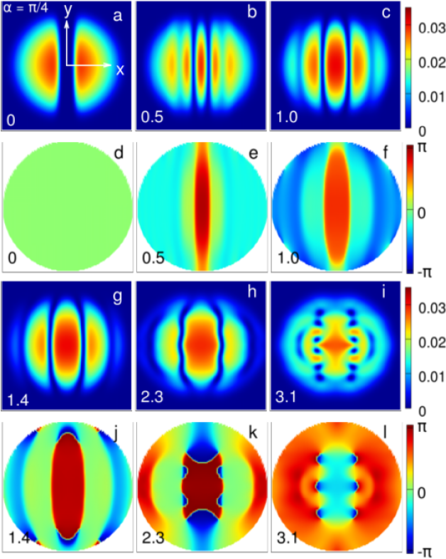
Figure 2: Merging dynamics of two fragments of the DBEC along the $x$-axis (directed along the horizontal direction in each image) for $\alpha=\pi/4$. The obstacle potential $V^{\perp}_{\rm obs}$ is switched off at $t=0~{}\omega^{-1}$. The first and third rows show the densities of the DBEC, while the third and fourth rows show the corresponding phases at different times. The time in units of $\omega^{-1}$ is shown at the bottom left corner of each image. The dimensions of each square image are $12~{}a_{\rm osc}\times 12~{}a_{\rm osc}$, and the origin is located at the center of each image.

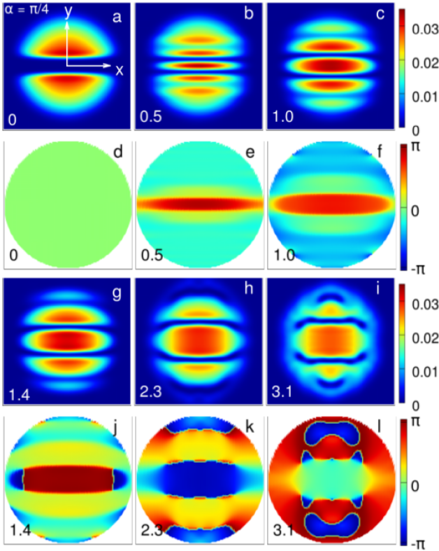
Figure 3: Merging dynamics of two fragments of the DBEC along the $y$-axis (directed along the vertical direction in each image) for $\alpha=\pi/4$. The obstacle potential $V^{\parallel}_{\rm obs}$ is switched off at $t=0~{}\omega^{-1}$. The first and third rows show the densities of the DBEC, while the third and fourth rows show the corresponding phases at different times. The time in units of $\omega^{-1}$ is shown at the bottom left corner of each image. The dimensions of each square image are $12~{}a_{\rm osc}\times 12~{}a_{\rm osc}$, and the origin is located at the center of each image.

The energy of the DBEC without any obstacle potential is $8.11~{}\hbar\omega$. This energy does not include $\hbar\omega_{z}/2$ contribution form the axial direction which was neglected while writing Eq. (6) as has been mentioned in the introduction. We find that energy cost of splitting the condensate along the $y$-axis is greater than splitting it along the $x$-axis; the energy difference $\Delta E=0.24~{}\hbar\omega$ for the system studied in Fig. 2(a) ($E=9.96~{}\hbar\omega$) and Fig. 3(a) ($E=9.72~{}\hbar\omega$). In case the dipoles are not oriented along the $z$-axis, the dispersion relation has a directional dependence and for a homogeneous two dimensional system is given by Fischer ; Ticknor

$$\omega_{\rm 2d}(\mathbf{k}_{\rho}) = \Bigg{\{}\frac{k_{\rho}^{4}}{4}+2nNk_{\rho}^{2}\sqrt{2\pi\lambda_{z}}\bigg{[}a+a_{\rm dd}\Big{(}\cos^{2}(\alpha)h^{\perp}_{\rm 2d}$$ (10)

$$+\sin^{2}(\alpha)h^{\parallel}_{\rm 2d}\Big{)}\bigg{]}\Bigg{\}}^{1/2}.$$

The Bogoliubov dispersion obtained using this expression for $n=0.035$ (peak density corresponding to images in Fig. 2 and Fig. 3), $N=5.0\times 10^{4}$, $\lambda_{z}=98$, and $\alpha=\pi/4$ is shown in Fig. 4.

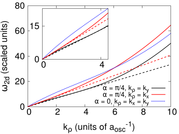
Figure 4: The solid red and black lines are the Bogoliubov dispersion for the excitations propagating along the $x$- and $y$-axis respectively for $\alpha=\pi/4$. The dashed red line is the tangent to these dispersion curves; its slope is equal to the speed of sound. The slope of the dashed black curve is equal to the Landau critical velocity along the $y$-axis. The dotted blue is the isotropic Bogoliubov dispersion for $\alpha=0$. For all the curves $n=0.035$, $N=5\times 10^{4}$, and $\lambda_{z}=98$. Inset shows the zoom-in of the main figure.

Also, the speed of the sound

$$c_{\rho} = \lim_{k_{\rho}\rightarrow 0}\frac{\omega_{\rm 2d}(\mathbf{k}_{\rho})}{k_{\rho}},$$ (11)

$$= \sqrt{2nN\sqrt{2\pi\lambda_{z}}[a+a_{\rm dd}(2\cos^{2}\alpha-\sin^{2}{\alpha})]},$$

and hence is isotropic. This is in contrast to three dimensional (homogeneous) DBEC where the speed of the sound Lahaye-2 ; Lima ; Muruganandam

$$c_{\rho}=\sqrt{\frac{nN}{m}\left[g+\frac{C_{\rm dd}}{3}(3\cos^{2}\Theta-1)\right]},$$ (12)

where $\Theta$ is the angle between the wavevector and the direction of polarization. Hence, the speed of the sound in three dimensional DBEC is anisotropic and it has been demonstrated experimentally Bismut-1 . Now, applying $V^{\parallel}_{\rm obs}$ leads to large density variations along the $y$-axis producing excitations that lie on the black curve in Fig. 4 including the roton-like mode. In the present work, we use the term roton-like mode to refer to the relative softening of the dispersion for the quasi-particle propagation perpendicular to the tilt of the dipoles on the plane of the condensate as compared to the dispersion perpendicular to it Ticknor . The relative softening at the intermediate momentum results in the inflection point on the dispersion curve (see the inset of Fig. 4) without leading to typical roton minimum Santos , which can not arise in a quasi-two dimensional condensate PB_Blakie . On the other hand, applying $V^{\perp}_{\rm obs}$ leads to large density variations along the $x$-axis which can excite only modes with energy greater than the roton-like mode as is evident from the red curve in Fig. 4. Thus, the anisotropic response of the condensate to the perturbing potential is another manifestation of the anisotropic dispersion and roton-like mode in the excitation spectrum, which makes the quasi-particle excitations along the $y$-axis cost less energy. Now, in order to allow the two fragments of the DBEC to merge non-adiabatically, we suddenly switch off the obstacle potentials. This leads to the generation of a train of dark notches. We identify these dark notches as solitons. The reasons for this identification are as follows. The dark solitons in quasi-two-dimensional condensates exhibit two competing instability mechanisms Carr . Firstly, a long wavelength sinusoidal mode transverse to the soliton grows exponentially, deforming the dark soliton into a snake like form. Later on, the arcs of this ‘snake’ like soliton decay into vortex-antivortex pairs. This instability, known as snake instability Kadomtsev ; Jones , has nothing to with the presence of the trapping potential and even occurs in the homogeneous two- and three-dimensional condensates. Secondly, a dark soliton propagates at the fraction of the speed of the sound which depends on its depth, and the speed of the sound is directly proportional to the square root of the density of the condensates Dalfovo . Hence, in the presence of the trapping potential, the inhomogeneous density profile causes the soliton to travel more slowly at the edges of the condensate than the center. As a result of it, an initially straight soliton formed near the center of the trap deforms into a curved shape Carr . We find that during the initial stages of the merging dynamics, the solitons become curved due to the inhomogeneity driven instability as is evident from Figs. 2(b), (c), (g) and Figs. 3(b), (c), (g). The increase in the curvature of the solitons is even more discernible in the phase plots shown in Figs. 2(e), (f), (j) and Figs. 3(e), (f), (j). After some time has elapsed, due to the snake instability the pair of the solitons near the trap center deforms into a sinusoidal shape as is evident from the Fig. 2(h) and Fig. 3(i). Moreover, the long lifetime, large amplitude, and phase structure of these dark notches also suggest their solitonic character. Our identification of these dark notches as the solitons is consistent with the experimental studies Dutton ; Chang ; Hau . These dark solitons are thus qualitatively different from the bright solitons in quasi-two dimensional DBECs which are stable and can move with a constant speed maintaining their shape Pedri ; Tikhonenkov ; R_Eichler . Now, the soliton train consists of four clearly discernible dark (grey) solitons. This is evident from Figs. 2(b), (c), (e), (f) and Figs. 3(b), (c), (e), and (f). We find that the separation between the adjacent solitons is not the same in the two cases considered. This is due to the fact that the solitons travel faster along the direction of polarization, i.e. the $x$-axis as compared to the $y$-axis. In order to clearly demonstrate this, we have measured the $x$ ($y$) coordinates of the mid-points of the solitons. The variations of these coordinates are shown by the red and green curves in Fig. 5. It is evident from this figure that solitons propagating along the $x$-axis travel faster than the ones propagating along the $y$-axis.

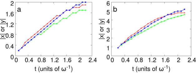
Figure 5: The red (green) curve is the $x$ ($y$) coordinate of the mid-point of the solitons shown in Fig. 2 (Fig. 3). The blue curve is the $x$ coordinate of the mid-point of the solitons shown in Fig. 8. Sub-figure (a) corresponds to the two solitons near to the origin, whereas the sub-figure (b) corresponds to the two solitons near the edge of the condensate.

We also observe that the solitons oriented along the direction of polarization are less susceptible to the snake instability as compared to the ones oriented perpendicular to it. This becomes clear by comparing Fig. 2(i), where the soliton pair near the trap center has already decayed into vortex-antivortex pairs, with Fig. 3(i), where the pair has only acquired a sinusoidal shape. This is due to the fact that the sinusoidal perturbation on the soliton oriented along the polarization direction costs more energy due to the anisotropy introduced by non zero value of $\alpha$. To confirm this inference, we have also numerically studied the dynamics of the DBEC which has a single dark soliton either along the $x$-axis or the $y$-axis. To do so, we first generate the soliton by imprinting a phase jump of $\pi$ across the $x$ or $y$-axis. The static solution thus obtained is shown in the first column of Fig. 6.

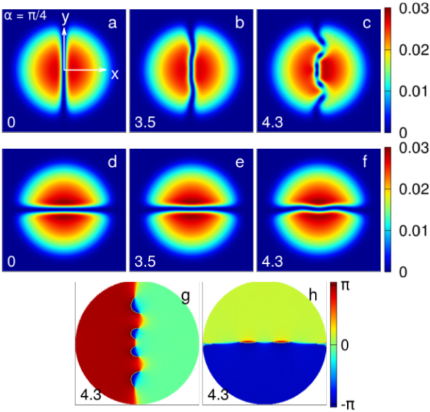
Figure 6: The upper (lower) row shows the dynamics of the dark soliton imprinted along the $y$ ($x$) axis for a given period. The sub-figures (g) and (h) are the phase plots corresponding to density distributions shown in sub-figures (c) and (f). The time in units of $\omega^{-1}$ is shown at the bottom left corner of each image. The dimensions of each image are $12~{}a_{\rm osc}\times 12~{}a_{\rm osc}$.

Again, as in the case of the obstacle potential, imprinting a soliton along the $x$-axis costs less energy due to the excitation of the roton like mode. We then evolve this solution in real time and find that by the time the soliton oriented along the $y$-axis acquires a sinusoidal shape due to snake instability, there is no perceptible change in the structure of the soliton oriented along the $x$ axis (see the middle column of Fig. 6). Later on at $4.3~{}\omega^{-1}$, when the soliton oriented along the $y$ axis has split into vortex-antivortex pairs due to the snake instability, the other soliton has merely acquired the sinusoidal shape due the snake instability as is shown in the last column of Fig. 6. The dipole-dipole interactions are also known to stabilize the three-dimensional dark solitons against the snake instability in the presence of an optical lattice in the nodal plane Nath . We have also studied the merging dynamics of a much larger condensate with $N=10^{5}$ with the rest of the parameters remaining unchanged. We find that for the larger condensate, the difference in the merging dynamics along the two orthogonal directions becomes more pronounced as is shown in Fig. 7, and hence can be easily verified in current experiments.

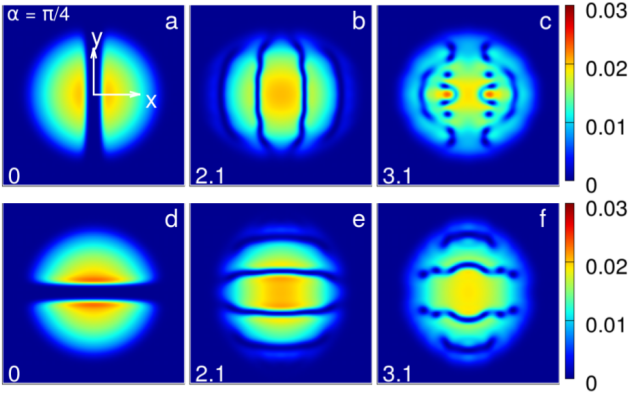
Figure 7: Merging dynamics of the DBEC with $10^{5}$ atoms. The time in units of $\omega^{-1}$ is shown at the bottom left corner of each image. The dimensions of each image are $16~{}a_{\rm osc}\times 16~{}a_{\rm osc}$.

This is due to the fact that by increasing $N$ while keeping the trapping potential parameters unchanged, density ($N|\phi|^{2}=Nn$) increases. This results in increasing the difference in the slopes of the two dashed curves in Fig. 4. In other words, the energy of the roton like mode is lowered, while the energy cost of exciting modes along $x$-axis increases. It implies that the anisotropy in the superfluidity of the system increases with the increase in the number of atoms. This leads to the significantly different merging dynamics along the $x$ and $y$-axes.

Isotropic merging: Here we consider $\alpha=0$, i.e. the dipoles are oriented along the $z$ axis and $N=5\times 10^{4}$. The trapping and obstacle potentials are the same as those considered in anisotropic merging dynamics. Again, we first obtain the static solution by solving Eq. (6) using imaginary time propagation for both obstacle potentials $V^{\perp}_{\rm obs}$ and $V^{\parallel}_{\rm obs}$. The solution thus obtained for the aforementioned barrier potential $V^{\perp}_{\rm obs}$ is shown in Fig. 8(a).

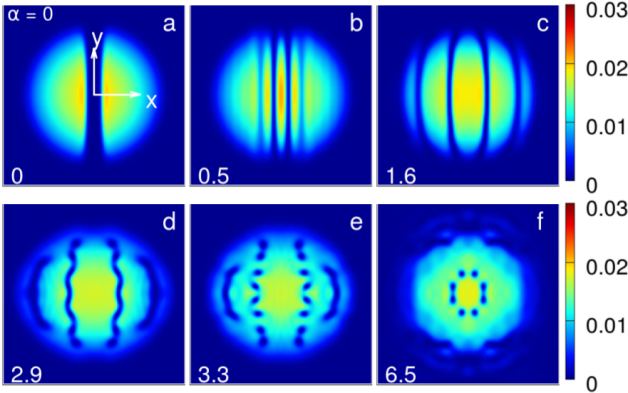
Figure 8: The merging dynamics of two fragments of dipolar condensates along the $x$ axis for $\alpha=0$. The time in units of $\omega^{-1}$ is shown at the bottom left corner of each image. The dimensions of each image are $16~{}a_{\rm osc}\times 16~{}a_{\rm osc}$.

We then suddenly switch off the obstacle potentials. This leads to the generation of a soliton train as in the previous case, which again consists of four clearly discernible dark (grey) solitons. This is evident from the Figs. 8(b), (c). We observe the exactly identical dynamics by using $V^{\parallel}_{\rm obs}$ instead of $V^{\perp}_{\rm obs}$. This is due to fact that the Bogoliubov quasi-particle dispersion obtained from Eq. 10 is isotropic for $\alpha=0$ as is shown by the dotted blue line in in Fig. 4 for $n=0.035$ and $N=5\times 10^{4}$. It is evident that the dispersion relation still has roton-like features, but no directional dependence. In other words, the roton like mode in this case is isotropic and hence the dynamics of merging is independent of direction.

III.2 Anisotropic splitting of the DBEC

In order to study the anisotropic splitting of the DBEC, we consider $5\times 10^{4}$ atoms of ⁵²Cr. In order to avoid the reflection of the DBEC from the edges of the grid, we consider a sufficiently large grid. The grid spacing, trapping potential and the scattering length values are same as those considered in the previous subsection. Here we first generate the static solution without any obstacle potential and consider $\alpha=\pi/4$. The static solution thus obtained is shown in Figs. 9(a) and (g).

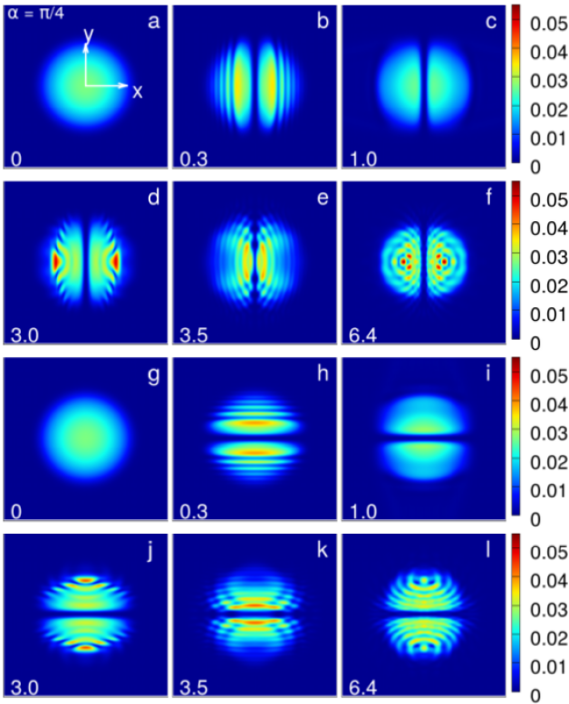
Figure 9: Anisotropic splitting dynamics of the DBEC. The time in units of $\omega^{-1}$ is shown at the bottom left corner of each image. The dimensions of each image are $16~{}a_{\rm osc}\times 16~{}a_{\rm osc}$.

We then suddenly introduce the obstacle potential either along the $x$ or $y$-axis. The strength and the width of the obstacle potentials are $50~{}\hbar\omega$ and $1~{}\mu$m respectively. The sudden turn-on of the obstacle potential produces sharp density gradients with several density peaks as is shown in Figs. 9(b) and (h), a possible signature of shock waves Hoefer . After some time, the broadest of these density peaks slowly grows at the expense of the others. During this period, the formation of the dispersive shock wave also leads to the spilling of some of the condensate atoms beyond the edge of the condensate (see Figs. 9(c) and (i)). We observe that during the initial stages of the evolution, the dynamics of splitting along the two orthogonal directions is almost identical as is evidenced by the comparison of Figs.9(b) and (c) with Figs. 9(h) and (i), respectively. The effect of anisotropy starts manifesting itself during the latter stages of evolution as is evidenced by a difference in the density distributions shown in Figs. 9(d), (e), and (f) vis-á-vis Figs. 9(j), (k), and (f). Hence, the dynamics of the splitting depends upon the direction along which the barrier is introduced. We also find that increasing the number of atoms to $10^{5}$ does not lead to any qualitative differences in the splitting dynamics. This may make it difficult to observe anisotropic splitting in current experiments. Also, the anisotropy in dynamics disappears for $\alpha=0$ as was the case for the merging dynamics.

IV Summary of results

We have numerically studied the dynamics of non-adiabatic merging and splitting of the dipolar Bose-Einstein condensate. The non-adiabatic merging and splitting is achieved by suddenly removing or applying an obstacle potential on the condensate. For the sake of observing the signature of anisotropic superfluidity, we implement the merging and splitting of the condensate along two orthogonal directions, one of which is parallel to the dipoles’ projection on the plane of the condensate. We observe that if the direction of polarization is not normal to the plane of the condensate, the roton-like features of the dispersion are manifested by the directional dependence of merging and splitting dynamics. The absence of the anisotropy in the merging and splitting dynamics rules out the existence of the anisotropic roton-like mode, although the isotropic roton like mode can still exist. From the experimental perspective, the tunability of the Bogoliubov dispersion by changing the density can be used to either increase or decrease the effects of anisotropic superfluidity on the dynamics of the DBEC. Our studies indicate that although anisotropic splitting may be difficult to observe experimentally, there should be no such issue with anisotropic merging dynamics.

- (1) A. Griesmaier, J. Werner, S. Hensler, J. Stuhler, and T. Pfau, Phys. Rev. Lett. 94, 160401 (2005); A. Griesmaier, J. Stuhler, and T. Pfau, Applied Physics B 82, 211 (2006).
- (2) T. Lahaye, T. Koch, B. Fröhlich, M. Fattori, J. Metz, A. Griesmaier, S. Giovanazzi, and T. Pfau, Nature 448, 672 (2007).
- (3) T. Koch, T. Lahaye, J. Metz, B. Fröhlich, A. Griesmaier, and T. Pfau, Nature Physics 4, 218 (2008).
- (4) T. Lahaye, C. Menotti, L. Santos, M. Lewenstein, and T. Pfau, Rep. Prog. Phys. 72, 126401 (2009).
- (5) M. A. Baranov, M. Dalmonte, G. Pupillo, and P. Zoller, Chem. Rev. 112, 5012 (2012).
- (6) M. Lu, N. Q. Burdick, S. H. Youn, and B. L. Lev, Phys. Rev. Lett. 107, 190401 (2011),
- (7) K. Aikawa, A. Frisch, M. Mark, S. Baier, A. Rietzler, R. Grimm, and F. Ferlaino, Phys. Rev. Lett. 108, 210401 (2012).
- (8) M. Lu, N. Q. Burdick, and B. L. Lev, Phys. Rev. Lett. 108, 215301 (2012).
- (9) K. Aikawa, A. Frisch, M. Mark, S. Baier, R. Grimm, and F. Ferlaino, Phys. Rev. Lett. 112, 010404 (2014).
- (10) J. Stuhler, A. Griesmaier, T. Koch, M. Fattori, T. Pfau, S. Giovanazzi, P. Pedri, and L. Santos, Phys. Rev. Lett. 95, 150 406 (2005).
- (11) G. Bismut, B. Pasquiou, E. Marećhal, P. Pedri, L. Vernac, O. Gorceix, and B. Laburthe-Tolra, Phys. Rev. Lett. 105, 040404 (2010).
- (12) L. Santos, G. V. Shlyapnikov, M. Lewenstein, Phys. Rev. Lett. 90, 250403 (2003).
- (13) R. M. Wilson, S. Ronen, J. L. Bohn, and H. Pu, Phys. Rev. Lett. 100, 245302 (2008).
- (14) R. M. Wilson, S. Ronen, and J. L. Bohn, Phys. Rev. Lett. 104, 094501 (2010).
- (15) L. Landau, J. Phys. (Moscow) 5, 71 (1941).
- (16) S. Yi and H. Pu, Phys. Rev. A 73, 061602(R) (2006).
- (17) S. Ronen, D. C. E. Bortolotti, and J. L. Bohn, Phys. Rev. Lett. 98, 030406 (2007).
- (18) R M. Wilson, S. Ronen, and J. L. Bohn, Phys. Rev. A 80, 023614 (2009).
- (19) P. B. Blakie, D. Baillie, and R. N. Bisset, Phys. Rev. A 86, 021604(R) (2012.
- (20) R. N. Bisset and P. B. Blakie, Phys. Rev. Let. 110, 265302 (2013).
- (21) J. P. Corson, R. M. Wilson, and J. L. Bohn, Phys. Rev. A 87, 051605 (2013).
- (22) J. P. Corson, R. M. Wilson, and J. L. Bohn, Phys. Rev. A 88, 013614 (2013).
- (23) M. Jona-Lasinio, K. Lakomy, and L. Santos, Phys. Rev. A 88, 025603 (2013).
- (24) A. Boudjemâa and G. V. Shlyapnikov, Phys. Rev. A 87, 025601 (2013).
- (25) M. Jona-Lasinio, K. Lakomy, and L. Santos, Phys. Rev. A 88, 013619 (2013).
- (26) U. R. Fischer, Phys. Rev. A 73, 031602(R) (2006).
- (27) C. Ticknor, R. M. Wilson, and J. L. Bohn, Phys. Rev. Lett. 106, 065301 (2011).
- (28) P. Muruganandam and S. K. Adhikari, Phys. Lett. A 376, 480 (2012).
- (29) G. Bismut, B. Laburthe-Tolra, E. Marećhal P. Pedri, O. Gorceix, and L. Vernac, Phys. Rev. Let. 109, 155302 (2012).
- (30) C. Ticknor, Phys. Rev. A 86, 053602 (2012).
- (31) J. J. Chang, P. Engels, and M. A. Hoefer, Phys. Rev. Lett. 101, 170404 (2008).
- (32) Z. Dutton, M. Budde, C. Slowe, and L. V. Hau, Science 293, 663 (2001).
- (33) J. A. Joseph, J. E. Thomas, M. Kulkarni, and A. G. Abanov, Phys. Rev. Lett. 106, 150401 (2011).
- (34) A. Bulgac, Y-L Luo, and K. J. Roche, Phys. Rev. Lett. 108 150401 (2012).
- (35) F. Ancilotto, L. Salasnich, and F. Toigo, Phys. Rev. A, 85, 063612 (2012).
- (36) W. Wan , S. Jia, and J. W. Fleischer, Nature Physics 3, 46 (2006).
- (37) A. Görlitz, J. M. Vogels, A. E. Leanhardt, C. Raman, T. L. Gustavson, J. R. Abo-Shaeer, A. P. Chikkatur, S. Gupta, S. Inouye, T. Rosenband, and W. Ketterle, Phys. Rev. Lett. 87, 130402 (2001).
- (38) P. Pedri and L. Santos, Phys. Rev. Lett. 95, 200404 (2005).
- (39) P. Muruganandam and S. K. Adhikari, Laser Physics 22, 813 (2012).
- (40) L. Salasnich, A. Parola, and L. Reatto, Phys. Rev. A 65, 043614 (2002).
- (41) W. Bao, D. Jaksch, and P. A. Markowich, J. Comp. Phys. 187, 318 (2003).
- (42) J. Werner, A. Griesmaier, S. Hensler, J. Stuhler, T. Pfau, A. Simoni, and E. Tiesinga Phys. Rev. Lett. 94, 183201 (2005).
- (43) R. M. Wilson and J. L. Bohn Phys. Rev. A 83, 023623 (2011).
- (44) R. Eichler, J. Main, and G. Wunner, Phys. Rev. A 83, 053604 (2011).
- (45) A. R. P. Lima and A. Pelster, Phys. Rev. A 86, 063609 (2012).
- (46) P. B. Blakie, D. Baillie, and R. N. Bisset, Phys. Rev. A 88, 013638 (2013).
- (47) Emergent Nonlinear Phenomena in Bose-Einstein Condensates: Theory and Experiment, edited by P. G. Kevrekidis, D. J. Frantzeskakis, and R. Carretero-Gonzalez (Springer-Verlag, Berlin, 2009).
- (48) B. B. Kadomtsev, V. I. Petviashvili, Sov. Phys. Dokl. 15, 539 (1970).
- (49) C. A. Jones, S. J. Putterman, P. H. Roberts, J. Phys. A 19, 2991 (1986).
- (50) F. Dalfovo, S. Giorgini, L. P. Pitaevskii, and S. Stringari, Rev. Mod. Phys. 71, 463 (1999).
- (51) L. V Hau, Nature Physics 3, 13 (2007).
- (52) I. Tikhonenkov, B. A. Malomed, and A. Vardi, Phys. Rev. Lett. 100, 090406 (2008).
- (53) R. Eichler, D. Zajec, P. Köberle, J. Main, and G. Wunner, Phys. Rev. A 86, 053611 (2012).
- (54) R. Nath, P. Pedri, and L. Santos, Phys. Rev. Lett. 101, 210402 (2008).
- (55) M. A. Hoefer, M. J. Ablowitz, I. Coddington, E. A. Cornell, P. Engels, and V. Schweikhard, Phys. Rev. A 74, 023623 (2006).