Phonon spectrum of QCD vacuum in magnetic-field-induced superconducting phase

Abstract

In the background of a sufficiently strong magnetic field the vacuum was suggested to become an ideal electric conductor (highly anisotropic superconductor) due to an interplay between the strong and electromagnetic forces. The superconducting ground state resembles an Abrikosov lattice state in an ordinary type–II superconductor: it is an inhomogeneous structure made of a (charged vector) quark-antiquark condensate pierced by vortices. In this paper the acoustic (phonon) vibrational modes of the vortex lattice are studied at zero temperature. Using an effective model based on a vector meson dominance, we show that in the infrared limit the longitudinal (transverse) acoustic vibrations of the vortex lattice possess a linear (quadratic) dispersion relation corresponding to type I (type II) Nambu–Goldstone modes.

I Introduction

The quantum vacuum may exhibit quite unusual properties in a strong magnetic field background if the magnetic field exceeds the hadronic-scale, $eB\gtrsim\Lambda_{\mathrm{QCD}}^{2}$. A strong magnetic field enhances the chiral symmetry breaking in QCD due to the magnetic catalysis phenomena ref:magnetic:catalysis . As a result, magnetic field affects the finite-temperature phase diagram of QCD ref:Tc:rising by shifting the transition temperature in a quite unexpected way ref:lattice:results . The phase structure of the QCD quark matter is also very sensitive to the presence of a strong magnetic field ref:magnetic:matter . In addition, the magnetized quark matter should exhibit new transport phenomena, such as the chiral magnetic effect ref:CME ; ref:CME:cond:matt , while the magnetic field background may affect standard transport phenomena ref:transport:related .

The interest in physics of extreme magnetic fields is justified by the fact that such strong fields may emerge in noncentral heavy-ion collisions. For example, in lead-lead collisions at the LHC, the strength of the generated magnetic field may reach $B\sim 10^{16}\,{\mathrm{T}}\sim 70m_{\pi}^{2}/e$ ref:field:estimation . The magnetic field may affect the quark-gluon plasma created by overlapping heavy ions as well as the vacuum between the ions if these ions near-miss each other in ultraperipheral collisions.

It was recently suggested that the strong magnetic field may cause the QCD vacuum to behave as an anisotropic perfect conductor (superconductor) at low temperatures Chernodub:2010qx ; Chernodub:2011mc if the strength of the magnetic field exceeds the critical value

$$B_{c}\simeq 10^{16}\,{\mathrm{Tesla}}\qquad{\mathrm{or}}\qquad eB_{c}\simeq 0.6\,\mbox{GeV}^{2}\,.\quad$$ (1)

The transition from the insulating to superconducting regimes is caused by the condensation of the quark-antiquark pairs, which carry the quantum numbers of the electrically charged $\rho$ mesons (we call it later “$\rho$-meson condensate”). The condensate is an anisotropic and inhomogeneous structure which may lack, in thermodynamics sense, a local order parameter beyond the mean field approximation ref:comment .

In contrast to the standard phenomenon of superconductivity the magnetic field penetrates the $\rho$ condensate: the Meissner effect is absent in the new phase because of the vector rather than scalar nature of the condensate Chernodub:2010qx .

This phenomenon has a known counterpart in the solid state physics which is sometimes the “reentrant” superconductivity ref:Zlatko . In an increasing magnetic field a type-II superconductor will eventually experience a transition to a normal phase and may then – according to the proposal of Ref. ref:Zlatko – “reenter” the superconducting regime again. The reentrant superconductivity is associated with an inhomogeneous $(p+ip)$ condensation of electron pairs and is suggested to be realized in certain materials. In the reentrant regime the emergent superconductivity does not screen the background magnetic field, while the breaking of the electromagnetic $U(1)$ symmetry results in appearance of short-range modulations (inhomogeneities) of the condensate in the transverse plane. In scope of the $\rho$–meson condensation the absence of the Meissner effect was discussed in Refs. Chernodub:2010qx , and a related proposal for ferromagnetic superconductors is put forward in Ref. ref:ferromagnetic .

Generally, a possible appearance of the $\rho$-meson condensate in strong magnetic field is not very surprising: it is quite similar to the gluon condensation in QCD ref:YM and to the $W$-boson condensation in the electroweak model ref:EW . The question on the possibility of $\rho$–meson condensation in high magnetic fields in QCD was also briefly raised in Ref. ref:earlier . Both $\rho$ mesons, gluons and $W$ bosons are vector particles, which are sensitive to high magnetic (chromomagnetic, in the case of gluons) fields. The closely related question of condensation of charged vector particles in the background of a magnetic field is discussed in Ref. ref:related:vector .

The condensation of quark-antiquark pairs with $\rho$–meson quantum numbers were also found in various holographic approaches ref:holographic ; ref:holographic:hexagonal , in local Chernodub:2011mc and nonlocal Frasca:2013kka Nambu–Jona-Lasinio (NJL) models as well as in numerical simulations of quenched lattice QCD Braguta:2011hq . Due to the anisotropic superconductivity the vacuum may become an exotic hyperbolic metamaterial which shares a similarity with diffractionless “perfect lenses” Smolyaninov:2011wc . The $\rho$–meson condensation is a subject of an ongoing discussion ref:comment ; ref:discussion .

In the mean field approach the vortices form a hexagonal lattice which is similar to the mixed Abrikosov state in an ordinary type–II superconductor. Since the vortex lattice breaks the continuous spatial symmetries, it should give rise to Nambu-Goldstone modes. These massless modes are, in fact, phonons which correspond to elementary vibrational excitations of the vortex lattice. The presence of phonons is crucial for understanding the stability of the vortex lattice against quantum and thermal fluctuations: depending on the spectrum of the phonon modes the vortex lattice may experience a chain of deformations and, eventually, melt into a vortex liquid ref:type-II:Review .

According to the numerical simulations of lattice QCD in strong magnetic field, the vortices appear in a liquid phase rather then in a form of the ordered vortex crystal Braguta:2013uc . Since the phonon modes are responsible for the melting of the vortex lattice (crystal), the study of the vortex excitations is physically interesting. In this paper we describe the vibrations of the $\rho$-vortex lattice following a well-developed calculation method for the phonon spectrum in Abrikosov vortex lattices in type II superconductors. A good review on this subject can be found in Ref. ref:type-II:Review .

In order to address the problem of the phonon spectrum of the vortex lattice we work in the framework of an effective electrodynamics for the $\rho$ mesons Djukanovic:2005ag based on the vector meson dominance Sakurai:1960ju . This model describes the superconducting ground state in consistency with other effective approaches ref:holographic ; ref:holographic:hexagonal ; Chernodub:2011mc ; Frasca:2013kka . The choice of this model is also justified by the analogy with usual superconductivity, where the standard Ginzburg-Landau approach describes well both the vortex-lattice ground state and its phonon excitations. Finally, we would like to mention that the use of the effective field theories in highly-magnetized zero-temperature QCD is generally supported by numerical lattice calculations. The relevant examples include a linear behavior of the chiral condensate (Refs. Shushpanov:1997sf and Bali:2012zg , respectively) and a peculiar nonlinear behavior of the chiral magnetization (Frasca:2011zn and Buividovich:2009ih respectively) as functions of magnetic field.

The structure of the paper is as follows. The effective electrodynamics of $\rho$ mesons and the ground state of this model in strong magnetic field are described in Section II. We introduce the basis of crystal wavefunctions and study their basic properties in Section III. In Section IV we derive the dispersion relation for the phonons. We show that in the infrared limit the transverse acoustic vibrations of the $\rho$-vortex lattice possess a quadratic “super-soft’ dispersion relation corresponding to type II Goldstone modes, while the longitudinal modes are always linear in momentum similarly to type I Goldstone bosons. Our main result for the dispersion relation for the low-energy phonons is given in Eq. (84):

$$\omega_{k}^{2} = k_{z}^{2}+f(B)\left({\boldsymbol{k}}^{2}\right)^{2}+\dots\,,$$ (2)

where $k_{z}$ and $\boldsymbol{k}$ are the longitudinal and transverse momenta, respectively, and the field-dependent prefactor $f(B)$ is given explicitly in Eq. (85). Apart from the prefactor, this dispersion relation for the low-energy phonons in the $\rho$-vortex ground state has the same qualitative form as the dispersion relation for the acoustic phonons in Abrikosov vortex lattices in conventional superconductors. The presence of the supersoft (quadratic) transversal mode in the phonon spectrum (2) may be responsible for the melting of the mean-field vortex lattice into the vortex liquid. The latter state was indeed observed in lattice simulations Braguta:2013uc . Our conclusions are given in the last section.

II Model, phases and approximations

The $\rho$ mesons are charged and neutral vector particles made of light ($u$ or $d$) quarks and antiquarks. A self-consistent quantum electrodynamics for the $\rho$ mesons can be described by the Djukanovic–Schindler–Gegelia–Scherer (DSGS) Lagrangian Djukanovic:2005ag :

$${\cal L} = -\frac{1}{4}\ F_{\mu\nu}F^{\mu\nu}-\frac{1}{2}\ \rho^{\dagger}_{\mu\nu}\rho^{\mu\nu}+m_{\rho}^{2}\ \rho_{\mu}^{\dagger}\rho^{\mu}$$

$$-\frac{1}{4}\ \rho^{(0)}_{\mu\nu}\rho^{(0)\mu\nu}+\frac{m_{\rho}^{2}}{2}\ \rho_{\mu}^{(0)}\rho^{(0)\mu}+\frac{e}{2g_{s}}\ F^{\mu\nu}\rho^{(0)}_{\mu\nu}\,,$$

where

$$\rho_{\mu}\equiv\rho^{-}=\frac{\rho^{(1)}_{\mu}-i\rho^{(2)}_{\mu}}{\sqrt{2}}\,,$$ (4)

and $\rho^{+}_{\mu}=\rho^{\dagger}_{\mu}$ are charged $\rho$ meson fields, $\rho^{(0)}_{\mu}$ is the neutral $\rho$ meson field and $A_{\mu}$ is the electromagnetic field. The field strengths in Eq. (II) are as follows:

$$F_{\mu\nu} = \partial_{\mu}A_{\nu}-\partial_{\nu}A_{\mu}\,,$$ (5)

$${f}^{(0)}_{\mu\nu} = \partial_{\mu}\rho^{(0)}_{\nu}-\partial_{\nu}\rho^{(0)}_{\mu}\,,$$ (6)

$$\rho^{(0)}_{\mu\nu} = {f}^{(0)}_{\mu\nu}-ig_{s}(\rho^{\dagger}_{\mu}\rho_{\nu}-\rho_{\mu}\rho^{\dagger}_{\nu})\,,$$ (7)

$$\rho_{\mu\nu} = D_{\mu}\rho_{\nu}-D_{\nu}\rho_{\mu}\,,$$ (8)

where $D_{\mu}=\partial_{\mu}+ig_{s}\rho^{(0)}_{\mu}-ieA_{\mu}$ is the covariant derivative and the phenomenological $\rho\pi\pi$ coupling is

$$g_{s}\equiv g_{\rho\pi\pi}\approx 5.88\,.$$ (9)

The $\rho$-meson mass at the vanishing magnetic field is $m_{\rho}(B=0)=775.5\,\mbox{MeV}$ and the mass of the neutral $\rho^{(0)}$ meson is as follows:

$$m_{0}\equiv m_{\rho^{(0)}}=m_{\rho}\Bigl{(}1-\frac{e^{2}}{g_{s}^{2}}\Bigr{)}^{-\frac{1}{2}}\,.$$ (10)

The DSGS model (II) is basically the vector meson dominance model Sakurai:1960ju coupled to electromagnetism with the following Abelian gauge transformations:

$$U(1)_{\mathrm{e.m.}}:\quad\left\{\begin{array}[]{lcl}\rho_{\mu}(x)&\to&e^{ie\omega(x)}\rho_{\mu}(x)\,,\\ \rho^{(0)}_{\mu}(x)&\to&\rho^{(0)}_{\mu}(x)\,,\\ A_{\mu}(x)&\to&A_{\mu}(x)+\partial_{\mu}\omega(x)\,.\end{array}\right.$$ (14)

We consider the model (II) in a background of a uniform static magnetic field parallel to the $x_{3}$ axis. The corresponding gauge potential is as follows:

$$A_{x}=-\frac{B}{2}y\,,\quad A_{y}=\frac{B}{2}x\,,\quad A_{z}=A_{t}=0\,.\quad$$ (15)

We ignore quantum fluctuations of the gauge and meson fields, thus treating the effective model (II) at the classical level. We always assume $eB>0$ for simplicity.

The model (II) predicts that if the magnetic field exceeds the critical value (1) then the vacuum enters a new phase where positively and negatively charged $\rho$–meson fields condense Chernodub:2010qx . In this phase the vacuum becomes a perfect electric conductor: the electric current can be carried by the $\rho$ condensates along the lines of the magnetic field without dissipation. The transport of electric charge along the magnetic field is described by a one-dimensional London equation, therefore we refer to the perfectly ideally conducting phase as “the superconductor phase” Chernodub:2010qx ; Chernodub:2011mc .

The electric superconductivity of the vacuum in strong magnetic field is caused by a $(p+ip)$–wave condensation of the charged $\rho$–meson field $\rho_{\mu}(x)\equiv\langle{\bar{u}}(x)\gamma_{\mu}d(x)\rangle$ with $\rho=\rho_{x}=-i\rho_{y}\neq 0$. Other vector components of the vector condensate are zero, $\rho_{z}=\rho_{t}=0$. In the mean–field approach and at the classical level of the effective model (II), the superconducting ground state of the vacuum resembles the Abrikosov lattice state in an ordinary type–II superconductor Chernodub:2011mc ; Chernodub:2010qx .

The mean-field solution for the ground state does not depend on the longitudinal $z$ coordinate. Therefore it is convenient to combine the transverse vectors into complex scalars: $\partial=\partial_{x}+i\partial_{y}$, ${\bar{\partial}}=\partial_{x}-i\partial_{y}$, or in general ${\cal O}={\cal O}_{x}+i{\cal O}_{y}$, ${\bar{\cal O}}={\cal O}_{x}-i{\cal O}_{y}$. As an exception to this general convention we put

$$\rho=\rho_{x}-i\rho_{y},$$ (16)

as the other combination simply vanishes in the LLL approximation:

$$\rho_{x}+i\rho_{y}\equiv 0\qquad({\mathrm{LLL}}).$$ (17)

The static (potential) energy density corresponding to the DSGS Lagrangian (II) is – assuming (17) – as follows:

$$\mathcal{E}_{\perp}[\rho,\rho_{0},A]=\frac{1}{2}|\mathcal{D}\rho|^{2}+\frac{1}{2}F_{xy}^{2}+\frac{1}{2}\bigl{(}\rho^{(0)}_{xy}\bigr{)}^{2}$$

$$\hskip 25.60747pt+\frac{1}{2}m_{\rho}^{2}\bigl{(}|\rho^{(0)}|^{2}+|\rho|^{2}\bigr{)}-\frac{e}{g_{s}}F_{xy}\rho^{(0)}_{xy}\,,$$ (18)

where

$$\mathcal{D}\rho = \partial\rho+ig_{s}\rho^{(0)}{\rho}-ieA{\rho},$$ (19)

$$F_{xy} = -\frac{i}{2}({\bar{\partial}}A-\partial{\bar{A}})\quad=B\ ,$$ (20)

$$\rho^{(0)}_{xy} = \frac{g_{s}}{2}|\rho|^{2}-\frac{i}{2}\bigl{(}\bar{\partial}\rho^{(0)}-\partial\bar{\rho}^{(0)}\bigr{)}.$$ (21)

We consider the spontaneous condensation of the $\rho$ meson fields in the background of the magnetic field (15) in the vicinity of the transition temperature: $B>B_{c}$ with $B-B_{c}\ll B_{c}$. One can show that in this case the $\rho$-meson condensate is very small, $|\rho|\ll m_{\rho}$, and the equations of motion for $\rho$-meson fields can be linearized Chernodub:2010qx . The smallness parameter is:

$$\epsilon=\frac{g_{s}|\rho|_{\mathrm{max}}}{m_{\rho}}\simeq\sqrt{\frac{B-B_{c}}{2B_{c}}},\qquad B>B_{c}\,,$$ (22)

where $|\rho|_{\mathrm{max}}\equiv\max_{z}|\rho(z)|$ is the maximal value of the inhomogeneous condensate of the $\rho$ field.

The classical equations of motion in the magnetic field background are discussed in details in Ref. Chernodub:2010qx . The equation for the charged $\rho$–meson condensate can be written as follows:

$$\mathcal{D}\rho=0\,,$$ (23)

where the correction to this equation is of the order of $\mathcal{O}(\epsilon^{4})$ with $\epsilon$ given in Eq. (22). Basically, the solutions of Eq. (23) reduce possible condensate solutions to the space of the lowest Landau levels.

The neutral $\rho$–meson field $\rho^{(0)}\equiv\rho^{(0)}_{x}+i\rho^{(0)}_{y}$ can be expressed via the charged $\rho$–meson condensate in the following form:

$$\rho^{(0)}=i\frac{g_{s}}{2}\frac{\partial}{-\Delta+m_{0}^{2}}|\rho|^{2}\,,$$ (24)

where $\Delta=\partial\bar{\partial}\equiv\partial^{2}_{x}+\partial^{2}_{y}$ is the two–dimensional Laplacian,

$$\frac{1}{-\Delta+m^{2}_{0}}(x_{\perp})=\frac{1}{2\pi}K_{0}(m|x_{\perp}|)\,,$$ (25)

is the two-dimensional Euclidean propagator of a scalar particle with the mass of the neutral vector meson (10) and $K_{0}$ is a modified Bessel function.

Using the equations of motion for our model (II), the mean energy density (18) can be expressed via a nonlocal function of the $\rho$–meson condensate $\rho$,

$$\langle\mathcal{E}_{\perp}[\rho,\rho_{0},A]\rangle = \frac{1}{2}B^{2}+\langle\mathcal{E}_{\perp}[\rho]\rangle\,,$$ (26)

$$\langle\mathcal{E}_{\perp}[\rho]\rangle = \frac{e^{2}}{8}\langle|\rho|^{2}\rangle^{2}+\frac{1}{2}(m_{\rho}^{2}-eB)\langle|\rho|^{2}\rangle$$ (27)

$$+\frac{g_{s}^{2}}{8}m_{\rho}^{2}\Bigl{\langle}|\rho|^{2}\frac{1}{-\Delta+m_{0}^{2}}|\rho|^{2}\Bigr{\rangle}\,,$$

where $\rho$ field is a minimum-energy solution of Eq. (23) and the brackets $\langle\dots\rangle$ denote the average over the transverse plane:

$$\langle{\cal O}\rangle=\frac{1}{{\mathrm{Area}}_{\perp}}\int dxdy\,{\cal O}(x,y)\,,$$ (28)

and ${\mathrm{Area}}_{\perp}$ is the area of the transverse plane.

The ground state solution of the $\rho$ condensate in the $B>B_{c}$ phase is given by the following expression Chernodub:2011gs ,

$$\rho(x,y) = \sum_{n\in{\mathbb{Z}}}C_{n}h_{n}(x,y)\,,$$ (29)

where

$$h_{n}(x,y)=\exp\left\{-\pi\frac{(x-n\nu L_{B})^{2}{-}iy(x-2n\nu L_{B})}{L_{B}^{2}}\right\}\!,\qquad$$ (30)

are the eigenstates corresponding to the Lowest Landau Level and

$$L_{B}=\sqrt{\frac{2\pi}{eB}}$$ (31)

is the magnetic length.

The parameters $C_{n}$ and $\nu$ should be chosen to minimize the energy (27) gained due to the condensation of the $\rho$–meson fields (the condensation energy), at a fixed value of magnetic field. The minimization of the energy functional is usually done by assuming that the (generally, complex) parameters obey the symmetry $C_{n}=C_{n+N}$ for an integer $N$.

The global minimum of the energy functional (27) corresponds to a global minimum of the dimensionless quantity

$$\beta_{\rho}=\left\langle\frac{|\rho^{2}|}{\langle|\rho^{2}|\rangle}\,\frac{m_{0}^{2}}{-\Delta+m_{0}^{2}}\frac{|\rho^{2}|}{\langle|\rho^{2}|\rangle}\right\rangle\,,$$ (32)

which is an analogue of the Abrikosov ratio

$$\beta_{A}=\langle|\phi|^{4}\rangle/\langle|\phi|^{2}\rangle^{2}\,,$$ (33)

used in the Ginzburg-Landau theory of ordinary superconductors Chernodub:2011gs . Notice that $\beta_{\rho}\to\beta_{A}$ the limit $m_{0}\to\infty$.

In Ref. Chernodub:2011gs we have found that the condensation energy density (27) – with $\langle{\cal E}\rangle$ given in Eq. (27) – is minimized for $N=2$ with $C_{0}=iC_{1}$ and

$$\nu=\frac{\sqrt[4]{3}}{\sqrt{2}}=0.9306\dots\,.$$ (34)

This choice of the parameters corresponds to an equilateral triangular (called also hexagonal) lattice with $N=2$, similarly to the case of the Abrikosov lattice in the Ginzburg–Landau model. All lattices with odd values of $N$ possess higher energies than the $N=2$ case while all even–$N$ lattices are reduced to the $N=2$ case.

The parameters of Eq. (29) corresponding to the ground state are as follows:

$$C_{n}=C_{0}\,\alpha_{n},\quad\alpha_{2\mathbb{Z}}=1,\quad\alpha_{2\mathbb{Z}+1}=i\,.$$ (35)

The overall coefficient $C_{0}=C_{0}(B)$ of the solution (29) and (35) can then be calculated by a requirement of the minimization of the condensation energy (27) or the $\beta_{\rho}$ ratio (32). The mean-field behavior of the coefficient $C_{0}$ is calculated in Ref. Chernodub:2011gs and is also presented in Eq. (III.3).

It was numerically found that in the ground state close to the critical magnetic field (1) at $B=1.01B_{c}$ the ratio (32) takes the following value Chernodub:2011gs :

$$\beta_{\rho}(B=1.01B_{c})=1.0192\dots\,.$$ (36)

The $\rho$–meson condensate is an inhomogeneous function of the transverse coordinates $x$ and $y$ and is independent of the longitudinal $z$ coordinate (29). The inhomogeneities are caused by the presence of an infinite periodic lattice of the so-called $\rho$ vortices which are parallel to the magnetic field. The $\rho$–vortex is a stringy topological defect in the $\rho$ condensate as the phase of the $\rho$ field winds by $2\pi$ around the vortex center. There is one $\rho$ vortex per unit area $L_{B}^{2}=2\pi/|eB|$ of the transverse plane. According to calculations in DSGS model Chernodub:2011gs , supported also by the holographic models Bu:2012mq , the vortices arrange themselves in the transverse plane in the form of a hexagonal (equilateral triangular) lattice, Fig. 1. The hexagonal periodic lattice is encoded in the particular form of the parameters $\alpha_{n}$ and $\nu$ in Eq. (35).

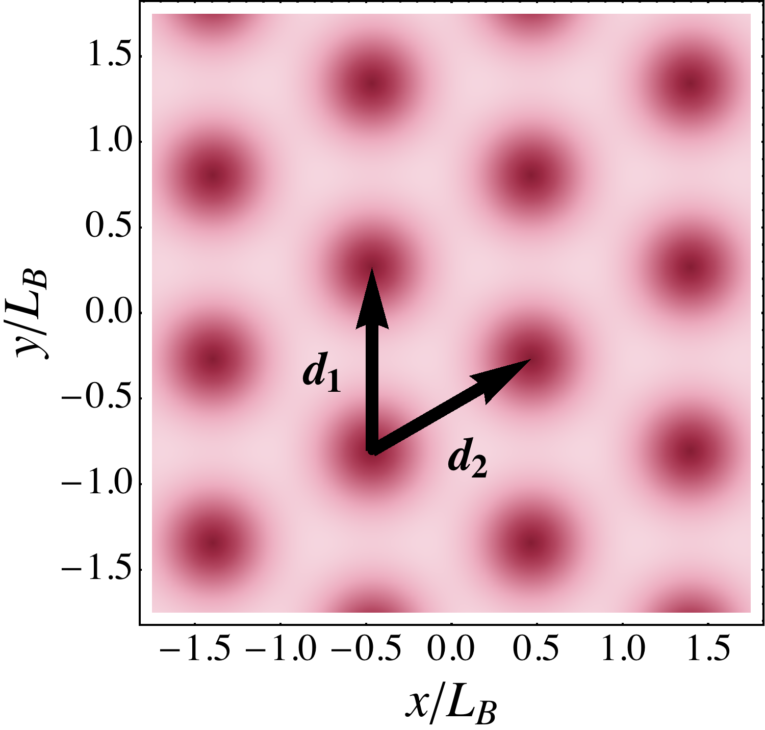
Figure 1: The density plot of the $\rho$–meson condensate (29) in the ground state. The coordinates are given in terms of the magnetic length (31). The darker regions corresponds to positions of the $\rho$ vortices where the superconducting density is small ($\rho\equiv 0$ at the centers of the vortices). In the mean-field ground state the vortices form the hexagonal lattice with the basic lattice vectors ${\boldsymbol{d}}_{1}$ and ${\boldsymbol{d}}_{2}$, Eq. (37).

For the hexagonal lattice solution (29) the basic lattice vectors are as follows:

$${\boldsymbol{d}}_{1}=\frac{L_{B}}{\nu}\left(0,1\right)\,,\qquad{\boldsymbol{d}}_{2}=\frac{L_{B}}{\nu}\left(\frac{\sqrt{3}}{2},\frac{1}{2}\right)\,.$$ (37)

The solution (29) is periodic, up to a phase factor, with respect to the shifts ${\boldsymbol{d}}_{1}$ and ${\boldsymbol{d}}_{2}$:

$$\rho({\boldsymbol{x}}+{\boldsymbol{d}}_{a}) = e^{i\pi{\boldsymbol{x}}\times{\boldsymbol{d}}_{a}/L_{B}^{2}}\rho({\boldsymbol{x}})\,,\qquad a=1,2\,,$$ (38)

where ${\boldsymbol{a}}\times{\boldsymbol{b}}=a_{i}\epsilon_{ij}b_{j}\equiv a_{x}b_{y}-a_{y}b_{x}$ is the vector product, and the latin superscript $a$ labels the basic vectors (37).

III Crystal wavefunctions

III.1 Definition

According to Eq. (38), the ground state solution (29), (30), (35) is not invariant under the translational shifts along basic vectors (37) in the transverse plane. In order to study the vibrations of the vortex lattice it is convenient to describe the full basis of the eigenstates of the Lowest Landau Level (30) by the so-called “magnetically translated” states. We follow the standard procedure which is used to study the vibrations of the vortex lattice in usual superconductors ref:type-II:Review .

We will perturb the vortex lattice both in transverse and longitudinal dimensions by slightly deformed configurations carrying so called “crystal quasimomentum” $k=({\boldsymbol{k}},k_{z})$ where ${\boldsymbol{k}}=(k_{x},k_{y})$ and $k_{z}$ are the transverse and longitudinal quasimomenta, respectively. These quasimomentum states are space dependent functions, close to the original lattice configuration, but shifted to hold a relative momentum in a special way ref:type-II:Review :

$$\begin{array}[]{rcl}\rho_{k}(\boldsymbol{x},z)&=&e^{ik_{z}z}\rho_{\boldsymbol{k}}(\boldsymbol{x})\,,\\[2.84526pt] \rho_{\boldsymbol{k}}(\boldsymbol{x})&=&e^{i\boldsymbol{k}\boldsymbol{x}}\psi_{\boldsymbol{k}}(\boldsymbol{x})\,,\end{array}$$ (41)

where

$$\psi_{\boldsymbol{k}}(\boldsymbol{x})=\rho\Bigl{(}{\boldsymbol{x}}+\frac{2{\tilde{\boldsymbol{k}}}}{eB}\Bigr{)}\equiv\rho\Big{(}{\boldsymbol{x}}+\frac{L_{B}^{2}}{\pi}{\tilde{\boldsymbol{k}}}\Big{)}\,,$$ (42)

and ${\tilde{k}}_{i}=\epsilon_{ij}k_{j}$ is the conjugate momentum. The shifted ground state function $\psi_{\boldsymbol{k}}$ satisfies the classical equations of motion, in particular, Eq. (23). By construction, the momentum states (41) and (42) satisfy the periodicity rule (38) for arbitrary momentum $\boldsymbol{k}$:

$$\rho_{\boldsymbol{k}}({\boldsymbol{x}}+{\boldsymbol{d}}_{a}) = e^{i\pi{\boldsymbol{x}}\times{\boldsymbol{d}}_{a}/L_{B}^{2}}\rho_{\boldsymbol{k}}({\boldsymbol{x}})\,,\qquad a=1,2\,.$$ (43)

The unperturbed ground–state function (29) corresponds to the function (41) with zero quasimomentum, $\rho\equiv\rho_{0}$.

It is convenient to define new dimensionless transversal coordinates:

$$\boldsymbol{x}^{\prime}=\frac{1}{L_{B}}{\boldsymbol{x}}\,,\qquad\boldsymbol{k}^{\prime}=\frac{L_{B}}{\pi}{\boldsymbol{k}}\,,$$ (44)

and then drop the primes, so that the the explicit form of the momentum eigenfunctions (41) is as follows:

$$\rho_{\boldsymbol{k}}(x,y) = e^{i\pi(xk_{x}+yk_{y})}\rho(x-k_{x},y+k_{y})$$

$$\equiv C_{0}e^{i\pi\left(\pi xy-k_{x}k_{y}\right)+2\pi iyk_{y}}$$

$$\cdot\sum_{n\in{\mathbb{Z}}}\alpha_{n}e^{-\pi(x-n\nu-k_{y})^{2}+2\pi in\nu y+2\pi in\nu k_{x}}.$$

In subsequent sections we will define the excited vortex states in terms of the quasimomentum wavefunctions (41). These wavefunctions will eventually enter the perturbed energy density (27), which consists of two– and four–point functions with respect to the average over the transverse space (28). For the sake of further convenience, in the rest of this section we define the two– and four–point functions of the quasimomentum wavefunctions (41) in the transverse plane. The dependence of the wavefunctions $\rho_{k}=e^{ik_{z}z}\rho_{\boldsymbol{k}}({\boldsymbol{x}})$ on the longitudinal coordinate $z$ is omitted below since it gives rise to trivial phase factors only.

It is well known that the periodicity of the functions (42) is inherited by the quasi-momenta, which can therefore be restricted to an elementary region in momentum space, the Brillouin-zone. This zone is then defined by the reciprocal vectors from $\boldsymbol{d}_{a}$ (37):

$$(\tilde{\boldsymbol{d}}_{a})_{i}=\frac{eB}{2}\epsilon_{ij}(\boldsymbol{d}_{a})_{j}\rightarrow\frac{1}{L_{B}}\epsilon_{ij}(\boldsymbol{d}_{a})_{j},$$ (46)

taking into account (44). While this periodicity allows a freedom in choosing the Brillouin zone, it is customary to choose it symmetrically around the origin and such that it respects the symmetries of the original lattice. In this way one can clearly identify the small momenta corresponding to the infrared regime we’re interested in. Since we are mainly interested in the infrared behavior of the phonon spectrum, in the remainder we will always assume all quasi-momenta sufficiently small, more explicitly:

$$k_{x},{l}_{x}\in\Big{[}-\frac{1}{4\nu},\frac{1}{4\nu}\Big{]},\quad k_{y},{l}_{y}\in\Big{[}-\frac{\nu}{2},\frac{\nu}{2}\Big{]}.$$ (47)

Given the symmetries of the system, one can extend the region above to a small hexagon inside the Brillouin zone as shown in Fig. 2. We have not tested the validity of our calculations outside this range, nor have we extended the calculations to include the full Brillouin zone. Since our results coincide in the limiting case of Abrikosov lattices with the known result, we expect good agreement in the whole Brillouin zone.

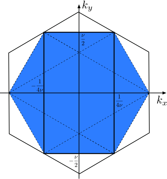
Figure 2: Brillouin zone in the transverse momentum space (outer hexagon) containing the range where our low momentum calculation holds (inner solid rectangle). Symmetries extend the latter rectangle to two rotated copies (dashed rectangles), combining to the inner (blue) hexagon part of the Brillouin zone for which our findings are valid.

III.2 Two-point function

The two-point function of the transverse wavefunctions $\rho_{\boldsymbol{k}}({\boldsymbol{x}})$ can be calculated explicitly using Eq. (III.1):

$$\bigl{\langle}\rho_{{\boldsymbol{l}}}^{*}\rho_{\boldsymbol{k}}\bigr{\rangle} = |C_{0}|^{2}\sum_{m,n\in{\mathbb{Z}}}\alpha_{n}\alpha_{m}^{*}e^{-\pi[(x-n\nu-k_{y})^{2}+(x-m\nu-{l}_{y})^{2}]}$$ (48)

$$\cdot e^{2i\pi\nu(n-m)y+2\pi i\nu(k_{x}n-{l}_{x}m)+2\pi i(k_{y}-{l}_{y})y}.\quad$$

By shifting the $x$ coordinate, $x\to x+n\nu+k_{y}$, we arrive to the following equation:

$$\bigl{\langle}\rho_{{\boldsymbol{l}}}^{*}\rho_{\boldsymbol{k}}\bigr{\rangle} = \frac{L_{B}^{2}|C_{0}|^{2}}{{\mathrm{Area}}_{\perp}}\int dxdye^{-2\pi x^{2}}\sum_{n\in{\mathbb{Z}}}|\alpha_{n}|^{2}e^{2\pi in\nu(k_{x}-{l}_{x})}\ \quad$$ (49)

$$= \frac{|C_{0}|^{2}}{\sqrt{2}\nu}\delta(\boldsymbol{k}-{\boldsymbol{l}})\,.$$

III.3 Four-point function

The (normalized) nonlocal correlation functions,

$$Q_{{\boldsymbol{l}}_{2},{\boldsymbol{k}}_{2},{\boldsymbol{l}}_{1},{\boldsymbol{k}}_{1}}=\frac{1}{|C_{0}|^{4}}\Big{\langle}\rho^{*}_{{\boldsymbol{l}}_{2}}\rho_{{\boldsymbol{k}}_{2}}^{~{}}\frac{M^{2}}{-\Delta+M^{2}}\rho^{*}_{{\boldsymbol{l}}_{1}}\rho_{{\boldsymbol{k}}_{1}^{~{}}}\Big{\rangle}\,,$$ (50)

correspond to the last term in the transverse energy functional (27). Inserting Eq. (III.1) into Eq. (50) and after an extensive algebra we find the following expression:

$$Q_{{\boldsymbol{l}}_{2},{\boldsymbol{k}}_{2},{\boldsymbol{l}}_{1},{\boldsymbol{k}}_{1}} = \frac{M^{2}}{2\nu^{2}}\sum_{m,n\in{\mathbb{Z}}}\frac{e^{-\pi\left(\boldsymbol{c}-\boldsymbol{X}_{m,n}\right)^{2}+2\pi i\epsilon_{ij}b^{i}X^{j}_{m,n}}}{4\pi^{2}\left(\boldsymbol{c}-\boldsymbol{X}_{m,n}\right)^{2}+M^{2}}$$ (51)

$$\equiv{\cal Q}(\boldsymbol{b},\boldsymbol{c},M)\,,$$

depending only on two linear combinations of the momenta $\boldsymbol{b}$ and $\boldsymbol{c}$ given below and the dimensionless mass

$$M=m_{0}L_{B}\,,$$ (52)

with $L_{B}$ is defined in Eq. (31). The vectors $\boldsymbol{b}$, $\boldsymbol{c}$ and ${\boldsymbol{X}}_{m,n}$ in Eq. (51) are as follows:

$$\boldsymbol{b} = \frac{\boldsymbol{k}_{1}+\boldsymbol{l}_{1}-\boldsymbol{k}_{2}-\boldsymbol{l}_{2}}{2}\,,$$ (53)

$$\boldsymbol{c} = \frac{\boldsymbol{l}_{1}-\boldsymbol{k}_{1}-\boldsymbol{l}_{2}+\boldsymbol{k}_{2}}{2}\,,$$ (54)

$$\boldsymbol{X}_{m,n} = m\,\tilde{\boldsymbol{d}}_{2}+n\,\tilde{\boldsymbol{d}}_{1}\,$$ (55)

$$= m\,\nu^{-1}\Big{(}\frac{1}{2}\boldsymbol{e}_{x}-\nu^{2}\boldsymbol{e}_{y}\Big{)}+n\,\nu^{-1}\boldsymbol{e}_{x}\,,$$ (56)

where $\boldsymbol{e}_{x}$ and $\boldsymbol{e}_{y}$ are the unit vectors in the $x$ and $y$ directions, respectively. A detailed calculation of the correlation function (51) is presented in Appendix A.

Notice that in our gauge (15) the function (51) is always a real function, which is even in both arguments:

$$Q_{{\boldsymbol{l}}_{2},{\boldsymbol{k}}_{2},{\boldsymbol{l}}_{1},{\boldsymbol{k}}_{1}}\equiv Q_{{\boldsymbol{k}}_{2},{\boldsymbol{l}}_{2},{\boldsymbol{k}}_{1},{\boldsymbol{l}}_{1}}\,,\quad{\mathrm{Im}}\,Q_{{\boldsymbol{l}}_{2},{\boldsymbol{k}}_{2},{\boldsymbol{l}}_{1},{\boldsymbol{k}}_{1}}=0\,.$$ (57)

One can check Eq. (51) by calculating the $\beta_{\rho}$ ratio (32):

$$\beta_{\rho}\equiv 2\nu^{2}Q_{0,0,0,0}=\sum_{m,n\in{\mathbb{Z}}}\frac{M^{2}e^{-\pi{\boldsymbol{X}}^{2}_{m,n}}}{4\pi^{2}{\boldsymbol{X}}^{2}_{m,n}+M^{2}}\,.$$ (58)

The $\beta_{\rho}$ ratio depends on magnetic field $B$ via the dependence of the mass parameter $M=M(B)$ according to Eqs. (31) and (52). An explicit calculation gives us that Eq. (58) at the critical magnetic field (1) reproduces the known numerical value (36). In the vicinity of the transition, $B\simeq B_{c}$, the parameter $\beta_{\rho}$ depends on the value of magnetic field $B$ very weakly. Parametrically,

$$\beta_{\rho}(B)=1.01937-0.01702\left(\frac{B}{B_{c}}-1\right)+\dots\,,$$ (59)

for $|B-B_{c}|\ll B_{c}$. In the limit $M\to\infty$ we recover the standard result $\beta_{A}=1.16$ for the value of the Abrikosov ratio for an equilateral triangular (hexagonal) lattice ref:type-II:Review .

Substituting the ground state wavefunction, Eq. (III.1) with ${\boldsymbol{k}}=0$, into the energy functional (27) we compute, term by term, the ground-state energy:

$$\mathcal{E}_{\perp}^{(0)} = \frac{e^{2}|C_{0}|^{4}}{16\nu^{2}}+\frac{m_{\rho}^{2}-eB}{2\sqrt{2}\nu}|C_{0}|^{2}$$ (60)

$$+\frac{g_{s}^{2}m_{\rho}^{2}}{8m_{0}^{2}}Q_{0,0,0,0}|C_{0}|^{4}\,,$$

where we used the definition (50).

The value of $|C_{0}|$ is then determined by the minimum of the energy (60). Given the phase degeneracy of the prefactor $C_{0}$ of the condensate $\rho_{0}$, we choose this prefactor to be a real number, $C_{0}=|C_{0}|$. Then the ground state for $B>B_{c}$ is defined by Eqs. (29), (30) and (35) with the prefactor

$$C_{0}(B) = \sqrt{\frac{2\sqrt{2}(eB-m_{\rho}^{2})\nu}{e^{2}+(g_{s}^{2}-e^{2})\beta_{\rho}}}$$

$$\simeq 0.2733\sqrt{eB-eB_{c}}\simeq 0.1504\sqrt{B-B_{c}}\,.$$

where we took into account the first equality in Eq. (58) and Eq. (10). In numerical estimation of the prefactor (III.3) we used $\alpha_{\mathrm{em}}\equiv e^{2}/4\pi=1/137$, the phenomenological value (9) for the coupling $g_{s}$, and the values (34) and (36) for, respectively, the parameter $\nu$ and for the $\beta_{\rho}$ ratio in the ground state.

Equation (60) allows us to compute the energy of the ground state at $B>B_{c}$:

$$\mathcal{E}_{\perp}^{(0)}(B)=-\frac{(eB-eB_{c})^{2}}{2[e^{2}+(g_{s}^{2}-e^{2})\beta_{\rho}]}$$ (62)

$$\qquad\simeq-0.0142(eB-eB_{c})^{2}\simeq-1.3\times 10^{-3}(B-B_{c})^{2}\,.$$

Obviously, in the low-$B$ phase the condensation energy is zero, $\mathcal{E}_{\perp}^{(0)}(B<B_{c})=0$.

IV Dispersion relation for phonons

We perturb the mean-field solution for the ground state (III.1), $\rho\equiv\rho_{\boldsymbol{0}}({\boldsymbol{x}})$, by adding the states which carry a nonzero quasimomentum $\boldsymbol{k}$ in the transverse plane:

$$\rho_{\mathrm{ph}}({\boldsymbol{x}})=\sum_{\boldsymbol{k}}\,c_{\boldsymbol{k}}\rho_{\boldsymbol{k}}({\boldsymbol{x}}),\qquad c_{|{\boldsymbol{k}}|\neq 0}\ll c_{0}=1\,.$$ (63)

Our strategy is to substitute the perturbed wavefunction (63) into the transverse energy functional (27), and expand the latter expression over the coefficients $c_{\boldsymbol{k}}$:

$$\mathcal{E}_{\perp}[\rho_{\mathrm{ph}}]=\mathcal{E}_{\perp}^{(0)}+\mathcal{E}^{(2)}_{\perp}+O(c_{\boldsymbol{k}}^{4})\,,$$ (64)

with $\mathcal{E}_{\perp}^{(0)}\equiv\mathcal{E}_{\perp}[\rho_{0}]$ is the ground state energy (62) and $\mathcal{E}^{(2)}_{\perp}\sim c_{\boldsymbol{k}}c_{\boldsymbol{k}^{\prime}}$ is the quadratic term of the phonon contribution to the energy. Then, the phonon eigenfunctions may be found by diagonalisation of the quadratic part $\mathcal{E}^{(2)}_{\perp}$ with respect to the coefficients $c_{\boldsymbol{k}}$.

IV.1 Propagation in the transverse plane

Due to the orthogonality of the magnetically translated wavefunctions (49) the quadratic term of the energy functional (27) is diagonal in the coefficients $c_{\boldsymbol{k}}$. However, the quartic term of this functional can, in general, mix four independent phonon modes of the perturbed wavefunction (63). Using the properties of the four-point function (57), one can show that number of independent mixing modes is reduced to a half of that upon complex conjugation. The mixing of the remaining two modes can be described by the following two-component vector,

$$v_{\boldsymbol{k}}=(c_{\boldsymbol{k}},c^{*}_{-{\boldsymbol{k}}})^{T}\,,$$ (65)

and the mixing term can be written as follows:

$$\Bigl{\langle}\rho^{*}\rho\frac{M^{2}}{-\Delta+M^{2}}\rho^{*}\rho\Bigr{\rangle}=\frac{1}{2}\sum_{{\boldsymbol{k}}}v^{\dagger}_{\boldsymbol{k}}\cdot{\hat{Q}}\cdot v_{\boldsymbol{k}}\,,$$ (66)

with the matrix

$${\hat{Q}}=2\left(\begin{array}[]{cc}Q_{{\boldsymbol{k}},{\boldsymbol{k}},0,0}+Q_{{\boldsymbol{k}},0,0,{\boldsymbol{k}}}&Q_{{\boldsymbol{k}},0,-{\boldsymbol{k}},0}^{*}\\ Q_{{\boldsymbol{k}},0,-{\boldsymbol{k}},0}&Q_{{\boldsymbol{k}},{\boldsymbol{k}},0,0}+Q_{{\boldsymbol{k}},0,0,{\boldsymbol{k}}}\end{array}\right).\qquad$$ (69)

The eigenvalues of the matrix (69) are as follows:

$$\lambda_{{\boldsymbol{k}},\pm} = 2\left(Q_{{\boldsymbol{k}},{\boldsymbol{k}},0,0}+Q_{{\boldsymbol{k}},0,0,{\boldsymbol{k}}}\pm|Q_{{\boldsymbol{k}},0,-{\boldsymbol{k}},0}|\right)$$ (70)

$$\equiv 2\left({\cal Q}({\boldsymbol{k}},0,M)+{\cal Q}(0,\boldsymbol{k},M)\pm|{\cal Q}(\boldsymbol{k},\boldsymbol{k},M)|\right),\qquad$$

Notice that

$$Q_{0,0,0,0}=\frac{\lambda_{0,+}}{6}=\frac{\lambda_{0,-}}{2}\equiv\frac{\beta_{\rho}}{2\,\nu^{2}}\,.$$ (71)

The eigenvectors of the matrix (69),

$$o_{\boldsymbol{k}}=\frac{c_{\boldsymbol{k}}+c_{-{\boldsymbol{k}}}^{*}}{2}\,,\qquad a_{\boldsymbol{k}}=\frac{c_{\boldsymbol{k}}-c^{*}_{-{\boldsymbol{k}}}}{2i}\,,$$ (72)

define the optical (massive) and acoustic (massless) phonon modes with the eigenvalues $\lambda_{{\boldsymbol{k}},+}$ and $\lambda_{{\boldsymbol{k}},-}$, respectively.

To the lowest order the energy functional of the optical and acoustic transverse modes reads as follows:

$$\mathcal{E}^{(2)}_{\perp}=\sum_{\boldsymbol{k}}\mathcal{E}^{(2)}_{\perp}({\boldsymbol{k}})\,,$$ (73)

where the contributions from the individual modes are diagonal in the coefficients $c_{\boldsymbol{k}}$:

$$\mathcal{E}^{(2)}_{\perp}({\boldsymbol{k}}) = c_{\boldsymbol{k}}^{*}c_{\boldsymbol{k}}\left(\frac{e^{2}}{4}\langle|\rho_{0}|^{2}\rangle\langle\rho_{\boldsymbol{k}}^{*}\rho_{\boldsymbol{k}}\rangle+\frac{1}{2}(m_{\rho}^{2}-eB)\langle\rho_{\boldsymbol{k}}^{*}\rho_{\boldsymbol{k}}\rangle\right)+\frac{g_{s}^{2}m_{\rho}^{2}|C_{0}|^{2}}{4\,m_{0}^{2}}\left(Q_{{\boldsymbol{k}},{\boldsymbol{k}},0,0}+Q_{{\boldsymbol{k}},0,0,{\boldsymbol{k}}}\right)c_{\boldsymbol{k}}c^{*}_{\boldsymbol{k}}$$

$$+\frac{g_{s}^{2}m_{\rho}^{2}|C_{0}|^{2}}{8}c_{\boldsymbol{k}}c_{-{\boldsymbol{k}}}Q_{0,{\boldsymbol{k}},0,-{\boldsymbol{k}}}+\frac{g_{s}^{2}m_{\rho}^{2}|C_{0}|^{2}}{8}{c_{\boldsymbol{k}}^{*}}c_{-{\boldsymbol{k}}}^{*}Q_{{\boldsymbol{k}},0,-{\boldsymbol{k}},0}$$

$$= o_{\boldsymbol{k}}^{2}\cdot\left(\frac{e^{2}}{8\nu^{2}}|C_{0}|^{2}+\frac{m_{\rho}^{2}-eB}{\sqrt{8}\nu}+\frac{g_{s}^{2}}{8}\frac{m_{\rho}^{2}}{m_{0}^{2}}|C_{0}|^{2}\lambda_{{\boldsymbol{k}},+}\right)+a_{\boldsymbol{k}}^{2}\cdot\left(\frac{e^{2}}{8\nu^{2}}|C_{0}|^{2}+\frac{m_{\rho}^{2}-eB}{\sqrt{8}\nu}+\frac{g_{s}^{2}}{8}\frac{m_{\rho}^{2}}{m_{0}^{2}}|C_{0}|^{2}\lambda_{{\boldsymbol{k}},-}\right).$$

The above expression can be simplified further using Eq. (71) and the fact that the parameter $C_{0}$, given explicitly in Eq. (III.3), corresponds to the minimum of energy (60):

$$\mathcal{E}^{(2)}_{\perp}({\boldsymbol{k}}) = \mathcal{E}^{(2)}_{\perp,O}({\boldsymbol{k}})+\mathcal{E}^{(2)}_{\perp,A}({\boldsymbol{k}})=\frac{g^{2}_{s}-e^{2}}{8}|C_{0}|^{2}$$ (75)

$$\cdot\Big{[}o_{\boldsymbol{k}}^{2}(\lambda_{{\boldsymbol{k}},+}-\lambda_{0,-})+a_{\boldsymbol{k}}^{2}(\lambda_{{\boldsymbol{k}},-}-\lambda_{0,-})\Big{]}\,.\quad$$

The phonon contribution to the transverse energy (75) has a massless mode in the $a_{\boldsymbol{k}}$ spectrum – the last term in Eq. (75) vanishes if ${\boldsymbol{k}}=0$ – which are therefore called the “acoustic” modes. The $o_{\boldsymbol{k}}$ modes represent the massive “optical” modes. Below we concentrate on massless acoustic modes.

According to Eqs. (75) and (71) the contribution of the acoustic modes to the energy can be rewritten as follows:

$$\mathcal{E}^{(2)}_{\perp,A}({\boldsymbol{k}})=a_{\boldsymbol{k}}^{2}\frac{g^{2}_{s}-e^{2}}{8}|C_{0}|^{2}\Big{(}\lambda_{{\boldsymbol{k}},-}-\frac{\beta_{\rho}}{\nu^{2}}\Big{)}\,,$$ (76)

with $C_{0}$ given in Eq. (III.3). The eigenvalue $\lambda_{{\boldsymbol{k}},-}$ is explicitly given by Eqs. (70) and (51):

$$\lambda_{-}({\boldsymbol{k}})\equiv\lambda_{\boldsymbol{k},-}=\frac{M^{2}}{2\nu^{2}}\Biggl{(}\sum_{\boldsymbol{X}}\frac{e^{-\pi(\boldsymbol{k}-\boldsymbol{X})^{2}}}{4\pi^{2}(\boldsymbol{k}-\boldsymbol{X})^{2}+M^{2}}$$ (77)

$$+\sum_{\boldsymbol{X}}\frac{e^{-\pi\boldsymbol{X}^{2}+2\pi i\boldsymbol{k}\times\boldsymbol{X}}}{4\pi^{2}\boldsymbol{X}^{2}+M^{2}}-\left|\sum_{\boldsymbol{X}}\frac{e^{-\pi(\boldsymbol{k}-\boldsymbol{X})^{2}+2\pi i\boldsymbol{k}\times\boldsymbol{X}}}{4\pi^{2}(\boldsymbol{k}-\boldsymbol{X})^{2}+M^{2}}\right|\Biggr{)}.$$

and $\boldsymbol{X}={\boldsymbol{X}}_{m,n}$ as given in Eq. (56) with $m,n\in{\mathbb{Z}}$ running over the whole lattice.

IV.2 Acoustic spectrum

The phonon contribution (76) to the energy is, in fact, a potential (time-independent) energy of essentially transverse modes with zero longitudinal momentum, $k_{z}=0$. The propagation in the longitudinal direction $z$ and the time evolution of the acoustic modes can naturally be taken into account by the following expression for the phonon fluctuations:

$$\rho_{\mathrm{ph}}({\boldsymbol{x}},z,t)=\sum_{{\boldsymbol{k}},k_{z}}\,c_{{\boldsymbol{k}},k_{z}}e^{-i\omega_{k}t+ik_{z}z}\rho_{\boldsymbol{k}}({\boldsymbol{x}})\,,$$ (78)

where $k=({\boldsymbol{k}},k_{z})$ according to Eq. (41).

The easiest way to obtain the dispersion relation for the phonon modes is to notice that the quadratic contribution to the time-dependent part of the Lagrangian (II) coming from the phonon fluctuations (78) is as follows:

$$T = \bigl{\langle}\mathcal{L}_{t}\bigr{\rangle}=\frac{1}{4}\bigl{\langle}|\partial_{t}\bar{\rho}|^{2}\bigr{\rangle}+\frac{1}{2}\bigl{\langle}|\partial_{t}\rho^{(0)}|^{2}\bigr{\rangle}$$ (79)

$$= \frac{\omega_{k}^{2}a_{k}^{2}}{4}\bigl{\langle}|\rho_{k}|^{2}\bigr{\rangle}=\frac{\omega_{k}^{2}a_{k}^{2}}{4\sqrt{2}\nu}\,.$$

The expression (79) plays a role of the kinetic energy of the phonon fluctuations. The potential energy is given by $V=\mathcal{E}^{(2)}_{\perp}({\boldsymbol{k}})+\mathcal{E}^{(2)}_{\|,A}(k_{z})$, where

$$\mathcal{E}^{(2)}_{\|,A}(k_{z})=\frac{a_{k}^{2}}{4\sqrt{2}\nu}k_{z}^{2}\,,$$ (80)

is the contribution from the longitudinal phonons which can be obtained by substituting the wavefunction of phonon fluctuations (78) into the expression for the full energy (18). Since the energy is diagonal in the longitudinal wavefunctions, there is no term which mixes the longitudinal modes with different $k_{\|}$.

Solving the equations of motion is then equivalent to putting $T-V=0$. Then we obtain the following dispersion relation for the acoustic phonon modes:

$$\omega_{k}^{2}=\frac{2e(g_{s}^{2}-e^{2})(B-B_{c})}{e^{2}+(g_{s}^{2}-e^{2})\beta_{\rho}}\left[\nu^{2}\lambda_{-}\!\!\left(\frac{L_{B}{\boldsymbol{k}}}{\pi}\right){-}\beta_{\rho}\right]\!{+}k_{z}^{2},\qquad$$ (81)

where the explicit form of $\lambda_{-}$ is given in Eq. (77). In deriving Eq. (81) we have used Eqs. (III.3) and (76).

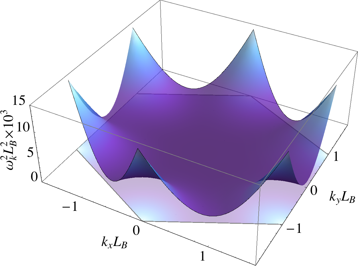
Figure 3: The dispersion $\omega_{k}$ of the gapless (photon) modes in the transverse momentum space, ${\boldsymbol{k}}=(k_{x},k_{y})$ at $B=1.01B_{c}$. The projection to $(k_{x},k_{y})$ plane corresponds to the Brillouin zone shown in Fig. 2.

The dispersion relation (81) for the transverse (with $k_{z}=0$) acoustic modes in the Brillouin zone is shown in Fig. 3. Qualitatively, the phonon spectrum in the $\rho$–vortex lattice is very similar to the spectrum of phonons in Abrikosov vortex lattices of conventional superconductors ref:type-II:Review .

IV.3 Low-energy spectrum of acoustic phonons

To obtain the infrared spectrum of the low-energy acoustic photons we expand the eigenvalue (77) over small transverse momenta ${\boldsymbol{k}}^{2}$:

$$\lambda_{-}(\boldsymbol{k})=\frac{\beta_{\rho}}{\nu^{2}}+\alpha(B)\left({\boldsymbol{k}}^{2}\right)^{2}+O\left(({\boldsymbol{k}}^{2})^{3}\right)\,,$$ (82)

$$\alpha(B=1.01B_{c})\simeq 0.662\,.$$ (83)

Similarly to the $\beta_{\rho}$ ratio (59), the prefactor (83) is practically insensitive to the magnetic field $B$ in the transition region.

In the case of the Abrikosov vortex lattice in a type–II superconductor – which is achieved by taking the limit $M\to\infty$ in Eq. (77) – the coefficient in front of the quartic term in Eq. (82) is 4 times bigger: $\alpha_{A}\simeq 2.72$.

Then we substitute the expansion (82) to the full phonon spectrum (81), and get the following infrared spectrum of the acoustic phonons:

$$\omega_{k}^{2} = k_{z}^{2}+f(B)\left({\boldsymbol{k}}^{2}\right)^{2}+\dots\,,$$ (84)

$$f(B) = \frac{C_{f}}{|eB|}\left(1-\frac{B_{c}}{B}\right)+\dots\,,$$ (85)

where $C_{f}\simeq 0.455$ and the higher-order corrections in ${\boldsymbol{k}}_{\perp}^{2}$ and in $B-B_{c}$ are shown by the ellipsis. This expansion is valid in the vicinity of the transition $B\geqslant B_{c}$.

The longitudinal part of the phonon spectrum (84) contains massless (“soft”) phonon modes with the linear dispersion relation $\omega_{{\boldsymbol{k}}=0,k_{z}}=k_{z}$. Thus, the acoustic phonons travel along the magnetic field axis with the speed of light and belong to type-I Nambu-Goldstone (NG) bosons.

The transverse part of the spectrum (84) corresponds to the “supersoft” phonon modes which are described by the quadratic dispersion relation $\omega_{{\boldsymbol{k}},k_{z}=0}=\sqrt{f(B)}{\boldsymbol{k}}^{2}$. This mode corresponds to a type-II NG boson. Similar quadratic dispersion relations were found for kaon condensation in the color-flavor locked phase of QCD at a nonzero strange chemical potential Schafer:2001bq ; Miransky:2001tw . Generalizations of the NG Amado:2013xya and pseudo-NG Filev:2009xp modes were found recently in the holographic approaches.

The purely transverse acoustic modes propagate with the following velocity (in units of speed of light $c$):

$$v_{\perp}({\boldsymbol{k}},k_{z}=0)=2\sqrt{f(B)}|{\boldsymbol{k}}|\,.$$ (86)

For example, at $B=1.01B_{c}$ a transverse acoustic phonon carrying energy $\omega_{{\boldsymbol{k}},0}=1$ MeV should travel with the velocity equal to 2% of speed of light.

The dispersion relation for the low-energy phonons (84) in the $\rho$-vortex lattices has the same qualitative form as the dispersion relation for the acoustic phonons in Abrikosov vortex lattices in conventional superconductors. As in the case of usual superconductors, the “super-softness” of the transverse phonon mode may lead to an instability of the $\rho$ vortex lattice against thermal and quantum fluctuations. Depending on the strength of these fluctuations, the superconductor’s vortex lattice may either withstand the perturbations or melt into either a vortex liquid ref:Moore or a vortex glass ref:Fischer (we refer a reader to the review ref:type-II:Review for further details). The study of stability of the vortex lattice is beyond the scope of this article.

V Conclusions

We have demonstrated the existence of the acoustic phonon modes in a suggested superconducting phase of QCD vacuum at strong magnetic field.

In the mean–field approach, the superconducting ground state resembles an Abrikosov vortex lattice in the mixed phase an ordinary type–II superconductor. The vortices are embedded in a vector quark-antiquark condensate with carries the quantum numbers of $\rho$ mesons. The vortices form a hexagonal lattice in the transverse plane with respect to the axis of the magnetic field. The lattice breaks translational and rotational symmetries of the coordinate space and leads to the appearance of the Nambu-Goldstone modes (acoustic phonons).

We have shown that the acoustic vibrations of the vortex lattice along the direction of the magnetic field is a linear function of momentum. A phonon propagating in the transverse plane possesses a quadratic (supersoft) dispersion relation in the limit of small momenta. The longitudinal phonons propagate with the speed of light while the velocity of their transverse counterparts depends on their energy and it may be much smaller than the speed of light. In the infrared limit the spectrum of acoustic phonons is given by Eq. (84).

The presence of the supersoft phonon modes is known to be crucial for the stability of the vortex lattice since these modes make an infrared divergent contribution to the free energy of the system ref:type-II:Review . As a result, the vortex lattice may become unstable and melt into a vortex liquid. In our paper we have found the supersoft mode in the phonon spectrum. This finding is in agreement with the results of the numerical simulations of lattice QCD in strong magnetic field background Braguta:2013uc which indicate the presence of the a liquid vortex state rather then an ordered vortex lattice.

Appendix A Explicit calculation of the quartic term

In this Appendix we evaluate the four–point function (50) which has the following explicit form:

$$Q_{{\boldsymbol{l}}_{2},{\boldsymbol{k}}_{2},{\boldsymbol{l}}_{1},{\boldsymbol{k}}_{1}} = \iint\frac{dxdy}{L_{x}L_{y}}\iint\frac{dx^{\prime}dy^{\prime}}{L_{x}L_{y}}$$

$$\prod_{i=1}^{2}\sum_{m_{i}\in{\mathbb{Z}}}\sum_{n_{i}\in{\mathbb{Z}}}M^{2}\delta(x-x^{\prime})f(y)\qquad$$

$$\hskip-59.75078pt\frac{\alpha h}{-\partial_{x}^{2}+4\pi^{2}[k_{1,y}-{l}_{1,y}+\nu(n_{1}-m_{1})]^{2}+M^{2}}g(x,x^{\prime})\,,$$

where $x^{\prime}$ is an arbitrary coordinate and

$$f(y) = e^{2\pi iy(k_{1,y}+k_{2,y}-l_{1,y}-l_{2,y})}$$

$$\cdot e^{2\pi iy\nu(n_{1}+n_{2}-m_{1}-m_{2})},$$

$$g(x,x^{\prime}) = e^{-\pi(x^{\prime}-\nu n_{2}-k_{2,y})^{2}-\pi(x^{\prime}-\nu m_{2}-l_{2,y})^{2}}$$

$$\cdot\,e^{-\pi(x-\nu n_{1}-k_{2,y})^{2}-\pi(x-\nu m_{2}-l_{2,y})^{2}},$$

$$h = e^{2\pi i\nu(k_{1,x}n_{1}+k_{2,x}n_{2}-{l}_{1,x}m_{1}-{l}_{2,x}m_{2})},$$

$$\alpha = \alpha_{m_{2}}^{*}\alpha_{m_{1}}^{*}\alpha_{n_{2}}\alpha_{n_{1}}.$$

We have assumed that we are working in a large but finite transverse space with dimensions $L_{x}\times L_{y}$. The derivative in Eq. (A) acts on the function $g(x,x^{\prime})$ only. For the sake of brevity, we do not show explicitly all arguments of the functions $f$, $g$, $h$ and $\alpha$ which are defined in Eq. (A).

The integral in Eq. (A) over the $y$ coordinate can be taken as follows. Firstly, one gets:

$$\int dyf(y) = \delta\bigl{(}k_{1,y}+k_{2,y}-l_{1,y}-l_{2,y}$$ (89)

$$+\nu(n_{1}+n_{2}-m_{1}-m_{2})\bigr{)}\,.$$

Because of the constraint we put on momenta in the $y$ direction (47), one finds that the absolute value of the sum $k_{1,y}+k_{2,y}-l_{1,y}-l_{2,y}$ in Eq. (89) should always be smaller than $2\nu$. Moreover, we need only the expressions with two nonzero momenta, so that the above sum turns out to be smaller than $\nu$. The later automatically implies $n_{1}+n_{2}-m_{1}-m_{2}=0$, so that

$$\int dyf(y) = \delta\left(k_{1,y}+k_{2,y}-l_{1,y}-l_{2,y}\right)$$ (90)

$$\cdot\,\delta_{n_{1}+n_{2}-m_{1}-m_{2}}.$$

The function $g(x,x^{\prime})$ in Eq. (A) can be rewritten as follows:

$$g(x,x^{\prime}) = e^{-\pi[(x+x^{\prime}-2r\nu-a_{y})^{2}+(x-x^{\prime}-2s\nu-b_{y})^{2}]}$$ (91)

$$\cdot\,e^{-\pi[(2t\nu+c_{y})^{2}+(2u\nu+d_{y})^{2}]}\,,$$

with

$$r =\frac{n_{1}+m_{1}+n_{2}+m_{2}}{2}\,, \boldsymbol{a} =\frac{\boldsymbol{k}_{1}+\boldsymbol{l}_{1}+\boldsymbol{k}_{2}+\boldsymbol{l}_{2}}{2}\,,$$

$$s =\frac{n_{1}+m_{1}-n_{2}-m_{2}}{2}\,, \boldsymbol{b} =\frac{\boldsymbol{k}_{1}+\boldsymbol{l}_{1}-\boldsymbol{k}_{2}-\boldsymbol{l}_{2}}{2}\,,$$

$$t =\frac{n_{1}-m_{1}-n_{2}+m_{2}}{2}\,, \boldsymbol{c} =\frac{\boldsymbol{l}_{1}-\boldsymbol{k}_{1}-\boldsymbol{l}_{2}+\boldsymbol{k}_{2}}{2}\,,$$

$$u =\frac{n_{1}-m_{1}+n_{2}-m_{2}}{2}\,, \boldsymbol{d} =\frac{\boldsymbol{l}_{1}-\boldsymbol{k}_{1}+\boldsymbol{l}_{2}-\boldsymbol{k}_{2}}{2}\,.$$

Equation (90) implies $u=d_{y}=0$. In terms of the new variables, we find $t=n_{1}-m_{1}$, $c_{y}=l_{1,y}-k_{1,y}$ and

$$h=e^{2\pi i\nu(ua_{x}+tb_{x}-rd_{x}-sc_{x})}\,.$$ (92)

To reproduce all possible integer values of $n_{1},\ldots m_{2}$ we use the following summation formula:

$$\tilde{\sum_{r,s,t}}\equiv\sum_{s,t\in\mathbb{Z}}\left(\sum_{r\in 2\mathbb{Z}+(s+t){\rm mod}2}\right)\,,$$ (93)

which takes into account the restriction $u=0$. An analysis of the $\alpha$–factor in Eq. (A) under the same conditions reveals that $\alpha=(-1)^{st}$.

We also rewrite the non-local operator in (A) as follows:

$$\frac{1}{-\partial_{x}^{2}+4(k_{1,y}-{l}_{1,y}+\pi\nu(n_{1}-m_{1}))^{2}+M^{2}}\delta(x-x^{\prime})$$ (94)

$$= \int dq\frac{e^{2\pi iq(x-\tilde{x})}}{4\pi^{2}q^{2}+4\pi^{2}(\nu t-c_{y})^{2}+M^{2}}\,.$$

Changing integration variables to

$$u=x+\tilde{x},\quad v=x^{\prime}-x,\quad dudv=2dxdx^{\prime},$$ (95)

and using all the above ingredients, the expression (A) becomes:

$$Q_{l_{2},k_{2},l_{1},k_{1}} = M^{2}\frac{\delta(d_{y})}{L_{x}L_{y}}\int dudvdq\tilde{\sum_{r,s,t}}(-1)^{st}e^{2\pi i[\nu(tb_{x}-rd_{x}-sc_{x})+qv]}\frac{e^{-\pi\left((u-r\nu-a_{y})^{2}+(v-s\nu-b_{y})^{2}+(t\nu-c_{y})^{2}\right)}}{q^{2}+4\pi^{2}(\nu t-c_{y})^{2}+M^{2}}$$ (96)

$$= M^{2}\frac{\delta(d_{y})}{L_{x}L_{y}}\int q\tilde{\sum_{r,s,t}}\mathbf{\alpha}e^{-2\pi i\nu(sc_{x}-sq+rd_{x})}\frac{e^{-\pi q^{2}-\pi(t\nu-c_{y})^{2}+2\pi i(\nu tb_{x}+qb_{y})}}{q^{2}+4\pi^{2}(\nu t-c_{y})^{2}+M^{2}}\,.$$

We will now take the $r$ summation and constrain $d_{x}$ to twice the region (47) as we will need at most two non-zero quasimomenta, i.e. $d_{x}$ should be smaller than $\frac{1}{2\nu}$:

$$\sum_{r\in 2\mathbb{Z}}e^{-2\pi i\nu rd_{x}} =\frac{1}{2\nu}\sum_{k}\delta(d_{x}-\frac{1}{2\nu}k)$$

$$\sum_{r\in 2\mathbb{Z}+1}e^{-2\pi i\nu rd_{x}} =\frac{1}{2\nu}\sum_{k}(-1)^{k}\delta(d_{x}-\frac{1}{2\nu}k)$$

$$\tilde{\sum_{s,t,r}}(-1)^{st}e^{-2\pi i\nu rd_{x}} =\frac{1}{2\nu}\sum_{r,s,t}(-1)^{r(s+t)+st}\delta(d_{x}-\frac{1}{2\nu}r)$$

$$=\frac{1}{2\nu}\sum_{s,t}(-1)^{st}\delta(d_{x})\,.$$

The $s$ summation gives likewise

$$\sum_{s}e^{-2\pi is\nu(c_{x}-q-\frac{t}{2\nu})} =\sum_{s}\frac{1}{\nu}\delta(q-c_{x}-\frac{1}{\nu}(s-\frac{1}{2}t))\,.$$

Using the identity $\delta(\boldsymbol{d}\,)\equiv L_{x}L_{y}$ we get:

$$Q_{l_{2},k_{2},l_{1},k_{1}}=\frac{M^{2}}{2\nu^{2}}\sum_{s,t}$$

$$\frac{e^{-\pi\left(c_{x}-\frac{2s-t}{2\nu}\right)^{2}-\pi(t\nu-c_{y})^{2}+2\pi i\left(\nu tb_{x}-b_{y}\frac{2s-t}{2\nu}\right)}}{4\pi^{2}\left(c_{x}-\frac{2s-t}{2\nu}\right)^{2}+4\pi^{2}(\nu t-c_{y})^{2}+M^{2}}\,,\qquad$$ (97)

where we have also used the following property:

$$e^{-i\pi(k_{1,x}k_{1,y}+k_{2,x}k_{2,y}-l_{1,x}l_{1,y}-l_{2,x}l_{2,y})}\delta({\boldsymbol{d}})=e^{-2\pi ib_{y}c_{x}}\delta({\boldsymbol{d}})\,.$$

Redefining $t\to-t$ in Eq. (97) we get the desired expression (51).

References

• (1) I. A. Shovkovy, Lect. Notes Phys.  871, 13 (2013); H. Suganuma and T. Tatsumi, Annals Phys.  208, 470 (1991); K. G. Klimenko, Z. Phys. C 54, 323 (1992); V. P. Gusynin, V. A. Miransky, I. A. Shovkovy, Phys. Rev. Lett.  73, 3499 (1994); Phys. Lett. B 349, 477 (1995); Nucl. Phys.  B462, 249 (1996).
• (2) N. O. Agasian and S. M. Fedorov, Phys. Lett. B 663, 445 (2008); R. Gatto, M. Ruggieri, Phys. Rev. D 82, 054027 (2010); Phys. Rev.  D 83, 034016 (2011); A. J. Mizher, M. N. Chernodub and E. S. Fraga, Phys. Rev. D 82, 105016 (2010); V. Skokov, Phys. Rev. D 85, 034026 (2012); V. D. Orlovsky and Y. A. Simonov, arXiv:1311.1087 [hep-ph]; J. O. Andersen, W. R. Naylor and A. Tranberg, arXiv:1311.2093 [hep-ph]; E. S. Fraga, B. W. Mintz and J. Schaffner-Bielich, arXiv:1311.3964 [hep-ph].
• (3) G. S. Bali, F. Bruckmann, G. Endrodi, Z. Fodor, S. D. Katz, S. Krieg, A. Schafer and K. K. Szabo, JHEP 1202, 044 (2012); F. Bruckmann, G. Endrodi and T. G. Kovacs, JHEP 1304, 112 (2013).
• (4) F. Preis, A. Rebhan and A. Schmitt, JHEP 1103, 033 (2011); J. Phys. G 39, 054006 (2012); V. Dexheimer, R. Negreiros and S. Schramm, Eur. Phys. J. A 48, 189 (2012); X. Kang, M. Jin, J. Xiong and J. Li, arXiv:1310.3012 [hep-ph].
• (5) K. Fukushima, D. E. Kharzeev and H. J. Warringa, Phys. Rev. D 78, 074033 (2008); M. A. Metlitski and A. R. Zhitnitsky, Phys. Rev. D 72, 045011 (2005).
• (6) A. Vilenkin, Phys. Rev. D 22, 3080 (1980). A. Yu. Alekseev, V. V. Cheianov, and J. Fröhlich, Phys. Rev. Lett. 81, 3503 (1998).
• (7) P. V. Buividovich, M. N. Chernodub, D. E. Kharzeev, T. Kalaydzhyan, E. V. Luschevskaya and M. I. Polikarpov, Phys. Rev. Lett.  105, 132001 (2010); N. O. Agasian, JETP Lett.  95, 171 (2012); S. -i. Nam and C. -W. Kao, Phys. Rev. D 87, 114003 (2013).
• (8) W. -T. Deng and X. -G. Huang, Phys. Rev. C 85, 044907 (2012); A. Bzdak and V. Skokov, Phys. Lett. B 710, 171 (2012).
• (9) M. N. Chernodub, Phys. Rev. D 82, 085011 (2010).
• (10) M. N. Chernodub, Phys. Rev. Lett.  106, 142003 (2011).
• (11) M. Frasca, JHEP 1311, 099 (2013).
• (12) M. N. Chernodub, Phys. Rev. D 89, 018501 (2014).
• (13) Z. Tesanovic, M. Rasolt and L. Xing, Phys. Rev. Lett. 63, 2425 (1989); M. Rasolt and Z. Tesanovic, Rev. Mod. Phys.  64, 709 (1992).
• (14) P. Olesen, arXiv:1311.4519 [hep-th].
• (15) J. Ambjorn and P. Olesen, Nucl. Phys. B 170, 60 (1980); Nucl. Phys. B 170, 265 (1980).
• (16) J. Ambjorn and P. Olesen, Nucl. Phys. B 315, 606 (1989); J. Ambjorn and P. Olesen, Phys. Lett. B 218, 67 (1989).
• (17) S. Schramm, B. Muller and A. J. Schramm, Mod. Phys. Lett. A 7, 973 (1992).
• (18) R. -G. Cai, S. He, L. Li and L. -F. Li, JHEP 1312, 036 (2013); R. -G. Cai, L. Li, L. -F. Li and Y. Wu, JHEP 1401, 045 (2014); R. -G. Cai, L. Li and L. -F. Li, JHEP 1401, 032 (2014).
• (19) M. Ammon, J. Erdmenger, P. Kerner and M. Strydom, Phys. Lett. B 706, 94 (2011); N. Callebaut, D. Dudal and H. Verschelde, JHEP 1303, 033 (2013); N. Callebaut and D. Dudal, JHEP 1401, 055 (2014).
• (20) Y. -Y. Bu, J. Erdmenger, J. P. Shock and M. Strydom, JHEP 1303, 165 (2013); K. Wong, JHEP 1310, 148 (2013).
• (21) V. V. Braguta, P. V. Buividovich, M. N. Chernodub, A. Y. Kotov and M. I. Polikarpov, Phys. Lett. B 718, 667 (2012).
• (22) I. I. Smolyaninov, Phys. Rev. Lett.  107, 253903 (2011).
• (23) M. N. Chernodub, Phys. Rev. D 86, 107703 (2012); Y. Hidaka and A. Yamamoto, Phys. Rev. D 87, 094502 (2013); C. Li and Q. Wang, Phys. Lett. B 721, 141 (2013).
• (24) B. Rosenstein and D. Li, Rev. Mod. Phys. 82, 109 (2010).
• (25) V. V. Braguta, P. V. Buividovich, M. Chernodub, M. I. Polikarpov and A. Y. Kotov, PoS ConfinementX 083, (2012) [arXiv:1301.6590 [hep-lat]].
• (26) I. A. Shushpanov and A. V. Smilga, Phys. Lett. B 402, 351 (1997).
• (27) G. S. Bali, F. Bruckmann, G. Endrodi, Z. Fodor, S. D. Katz and A. Schafer, Phys. Rev. D 86, 071502 (2012); P. V. Buividovich, M. N. Chernodub, E. V. Luschevskaya and M. I. Polikarpov, Phys. Lett. B 682, 484 (2010).
• (28) M. Frasca and M. Ruggieri, Phys. Rev. D 83, 094024 (2011).
• (29) P. V. Buividovich, M. N. Chernodub, E. V. Luschevskaya and M. I. Polikarpov, Nucl. Phys. B 826, 313 (2010).
• (30) D. Djukanovic, M. R. Schindler, J. Gegelia, S. Scherer, Phys. Rev. Lett.  95, 012001 (2005).
• (31) J. J. Sakurai, “Theory of strong interactions,” Annals Phys.  11, 1-48 (1960).
• (32) M. N. Chernodub, J. Van Doorsselaere and H. Verschelde, Phys. Rev. D 85, 045002 (2012).
• (33) Y. -Y. Bu, J. Erdmenger, J. P. Shock and M. Strydom, JHEP 1303, 165 (2013); K. Wong, JHEP 1310, 148 (2013) [arXiv:1307.7839 [hep-th]].
• (34) T. Schäfer, D. T. Son, M. A. Stephanov, D. Toublan and J. J. M. Verbaarschot, Phys. Lett. B 522, 67 (2001).
• (35) V. A. Miransky and I. A. Shovkovy, Phys. Rev. Lett.  88, 111601 (2002).
• (36) I. Amado, D. Arean, A. Jimenez-Alba, K. Landsteiner, L. Melgar and I. S. Landea, JHEP 1307, 108 (2013).
• (37) V. G. Filev, C. V. Johnson and J. P. Shock, JHEP 0908, 013 (2009).
• (38) M. A. Moore, Phys. Rev. B 39, 136 (1989)
• (39) M. P. A. Fisher Phys. Rev. Lett. 62, 1415 (1989).