Persistent charge and spin currents in a quantum ring using Green’s function technique: Interplay between magnetic flux and spin-orbit interactions

Abstract

We put forward a new approach based on Green’s function formalism to evaluate precisely persistent charge and spin currents in an Aharonov-Bohm ring subjected to Rashba and Dresselhaus spin-orbit interactions. Unlike conventional methods our present scheme circumvents direct evaluation of eigenvalues and eigenstates of the system Hamiltonian to determine persistent currents which essentially reduces possible numerical errors, especially for larger rings. The interplay of Aharonov-Bohm flux and spin-orbit interactions in persistent charge and spin currents of quantum rings is analyzed in detail and our results lead to a possibility of estimating the strength of any one of the spin-orbit fields provided the other one is known. All these features are exactly invariant even in presence of impurities, and therefore, can be substantiated experimentally.

I Introduction

The promise of new technological breakthroughs has been a major driving force for studying transport in meso- and nano-structures whose dimensions are comparable to and even smaller than the mean free paths or wavelengths of electrons datta1 ; imry1 ; datta2 . Simultaneously, inspection of electronic transport in low-dimensional systems comprising simple and complex structures has brought up several new underlying questions. The progress in experimental techniques has allowed for systematic investigations of artificially made nanostructures whose transport properties are affected or even governed by quantum effects and this makes it possible to perform experiments that directly probe quantum properties of phase coherent many-body systems.

The appearance of circular currents, induced by external magnetic fields in isolated (no source and drain electrodes) quantum rings, commonly known as persistent currents, is an astonishing quantum effect which reveals the significance of phase coherence of electronic wave functions in low-dimensional quantum systems. The phenomenon of persistent current in normal metal rings in presence of Aharonov-Bohm (AB) flux $\phi$ has been first exposed yang in the early $60$’s, and then, in $1983$ Büttiker et al. butt1 have successfully revived it and they have established that an isolated normal metal mesoscopic ring threaded by an AB flux $\phi$ carries an equilibrium current which does not decay over time and circulates within the sample. Following this pioneering work, interest in this subject has rapidly picked up with substantial theoretical gefen ; ambe ; schm1 ; schm2 ; bary ; maiti4 ; maiti5 ; maiti6 ; maiti7 ; maiti9 ; skm1 ; skm2 ; skm3 ; skm4 and experimental levy ; jari ; bir ; chand works. Still, many open questions persist in this particular issue. For instance, persistent current examined in disordered rings is considerably larger than the corresponding theoretical predictions chand ; mailly1 ; mailly . In $2009$, Bluhm et al. blu have made in situ measurements using scanning SQUID microscope for studying magnetic properties of $33$ discrete mesoscopic gold rings, taking one ring at a time. Their experimental results fit reasonably well with the theoretically predicted value gefen only in an ensemble of $16$ nearly ballistic rings mailly1 and in a single ballistic ring mailly . But, the current amplitudes in single isolated diffusive gold rings chand are still order of magnitude larger than the theoretical predictions. In presence of electron-electron (e-e) interaction and disorder an explanation has been proposed ambe ; smt ; mont ; ph , based on a perturbative calculation, which reveals persistent currents with greater amplitude compared to the non-interacting case, but still off by an order of magnitude. Moreover, the origin of the e-e interaction parameters taken into account in the theory is not suitably unraveled. Thus, it demands further studies to resolve these controversial issues.

Another challenging topic is the possible existence of a spin current qf1 in mesoscopic rings with spin-orbit (SO) interaction, even in the absence of a magnetic field. This phenomenon may be observed through the recently developed Doppler and spin modulation relaxation techniques vla ; and1 ; and2 . The SO interaction is a rudimentary mechanism that is manifested in several fascinating properties that pertain to the anticipations of semiconducting structures as potential quantum devices. In conventional semiconducting materials two typical SO interactions are encountered. One is called as Rashba spin-orbit interaction (RSOI) rash and the other is named as Dresselhaus spin-orbit interaction (DSOI) dress . The previous one is associated with electric field that is generated from the structural inversion asymmetry at interfaces, while the later results from the bulk inversion asymmetry gini . An additional contribution can also arise from surface anisotropies prem together with simple Rashba SO interaction, which is associated with the interfacial electric field normal to the surface that results from the band offset at the interface of two different semiconductors. Quantum rings - ring-shaped quantum wells fabricated at such heterojunctions - comprise such anisotropies are exemplary candidates for examining SO coupling effects in persistent currents. Note that if one of the components that make the interface is characterized by bulk asymmetry, a corresponding contribution of the DSOI will also exist at the interface wnk . In such quantum rings electronic transport will exhibit the interplay between these different contributions to the SO coupling at the interface. A sizable amount of related theoretical work has already revealed the distinctive features of persistent charge and spin currents in mesoscopic rings subjected to Rashba and Dresselhaus SO fields qf1 ; sng ; spl ; loss , however a well defined methodology for the prediction of persistent current in large samples is still missing and the magneto-transport properties of such structures are fascinating and remain controversial. The accurate determination of persistent current in such systems, in the presence of an AB flux, is a route for analyzing its magnetic properties.

A clear understanding of the role played by SO interactions in the phenomena of persistent charge and spin currents necessiates proper estimation of the strength of these interactions. The Rashba SO interaction which is controlled by an external gate voltage placed in the vicinity of the sample gini ; prem can be determined by the structure of the interface. This yields, in principle, a wide range of possible values of RSOI and its determination in any given material is crucial nit . The feasible routes of measuring the strength of DSOI are mainly based on the photo-galvanic methods yi , measurement of electrical conductance of nano-wires sc , and an optical monitoring of the spin precession of the electrons stu . A unitary transformation has been explored eg ; zh which brings out a hidden symmetry, when applied to the SO Hamiltonian, that has been used to establish that by making the strengths of the two SO interactions equal one achieves a zero spin current in the material maiti1 , and this vanishing spin current is a robust effect which is observed even in presence of disorder maiti1 , and thus, can be established experimentally. Observing the persistent charge current maiti2 one can estimate the strength of DSOI, and, by monitoring the vanishing of persistent spin current one can determine both the RSOI and DSOI in a single mesoscopic ring maiti1 ; maiti3 .

The established approach to the determination of persistent charge gefen ; spl ; maiti2 ; bouz ; giam ; yu ; maiti8 ; maiti10 ; skm5 and spin qf1 ; spl ; qf2 ; maiti3 currents in isolated conducting rings is based on the evaluation of eigenvalues and eigenvectors of the system Hamiltonian. For large size rings such an approach becomes highly numerically unreliable, and most importantly - hard to speculate in presence of interaction with external baths. Here we propose a new approach, based on Green’s function formalism, that circumvents the need to evaluate system eigenvalues and eigenfunctions. In particular, this Green’s function methodology for determining persistent currents should give us access to evaluation of the magnetic properties of large conducting rings as well as molecular rings encountered in biopolymers. We firmly believe that the Green’s function technique will yield persistent charge and spin currents a very high degree of accuracy, and this will definitely make it possible to consider the interplay between molecular structure and geometry and the resulting persistent currents obtained in the presence of an AB flux $\phi$ and SO interactions.

The rest of the paper is organized as follows. In Section II, the model quantum system and the calculation method are described. In Section III, the numerical results are presented which describe the (i) behavior of persistent charge current, (ii) characteristic features of persistent spin current, and (iii) possible route of estimating the strength of RSOI and DSOI in a single mesoscopic ring. Finally, in Section IV, we summarize our essential results.

II Theoretical framework

II.1 Model and Hamiltonian

We consider a mesoscopic ring which is subjected to both Rashba and Dresselhaus SO fields. The ring is threaded by an AB flux $\phi$ which is measured in unit of $\phi_{0}=ch/e$, the elementary flux-quantum. A schematic view of this ring is illustrated in Fig. 1.

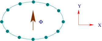
Figure 1: (Color online). Schematic representation of the model quantum system where a mesoscopic ring is threaded by an AB flux $\phi$. The filled circles correspond to the positions of the atomic sites.

The TB Hamiltonian of such a $N$-site ring in the site representation reads as maiti1 ; maiti2 ; maiti3 ,

$$\mbox{\boldmath$H$}_{\mbox{\tiny R}} = \sum_{n}\mbox{\boldmath$c_{n}^{\dagger}\epsilon_{n}c_{n}$}+\sum_{n}\left(\mbox{\boldmath$c_{n+1}^{\dagger}t$}\,e^{i\theta}\mbox{\boldmath$c_{n}$}+h.c.\right)$$ (1)

$$- \sum_{n}\left(\mbox{\boldmath$c_{n+1}^{\dagger}($}i\mbox{\boldmath$\sigma_{x})\alpha$}\cos\varphi_{n,n+1}\,e^{i\theta}\mbox{\boldmath$c_{n}$}+h.c.\right)$$

$$- \sum_{n}\left(\mbox{\boldmath$c_{n+1}^{\dagger}($}i\mbox{\boldmath$\sigma_{y})\alpha$}\sin\varphi_{n,n+1}\,e^{i\theta}\mbox{\boldmath$c_{n}$}+h.c.\right)$$

$$+ \sum_{n}\left(\mbox{\boldmath$c_{n+1}^{\dagger}($}i\mbox{\boldmath$\sigma_{y})\beta$}\cos\varphi_{n,n+1}\,e^{i\theta}\mbox{\boldmath$c_{n}$}+h.c.\right)$$

$$+ \sum_{n}\left(\mbox{\boldmath$c_{n+1}^{\dagger}($}i\mbox{\boldmath$\sigma_{x})\beta$}\sin\varphi_{n,n+1}\,e^{i\theta}\mbox{\boldmath$c_{n}$}+h.c.\right),$$

where, $\theta=2\pi\phi/N$ is the phase factor associated with the hopping of an electron between nearest-neighbor sites in presence of the AB flux $\phi$ and $\varphi_{n,n+1}=(\varphi_{n}+\varphi_{n+1})/2$, where $\varphi_{n}=2\pi(n-1)/N$. The other factors are defined as follows.
$c_{n}^{\dagger}$=$\left(\begin{array}[]{cc}c_{n\uparrow}^{\dagger}&c_{n\downarrow}^{\dagger}\end{array}\right),$ $c_{n}$=$\left(\begin{array}[]{c}c_{n\uparrow}\\ c_{n\downarrow}\end{array}\right),$ $\epsilon_{n}$=$\left(\begin{array}[]{cc}\epsilon_{n\uparrow}&0\\ 0&\epsilon_{n\downarrow}\end{array}\right),$
$t$=$t\left(\begin{array}[]{cc}1&0\\ 0&1\end{array}\right),$ $\alpha$=$\left(\begin{array}[]{cc}\alpha&0\\ 0&\alpha\end{array}\right),$ $\beta$=$\left(\begin{array}[]{cc}\beta&0\\ 0&\beta\end{array}\right),$
$\sigma_{x}$=$\left(\begin{array}[]{cc}0&1\\ 1&0\end{array}\right),$ $\sigma_{y}$=$\left(\begin{array}[]{cc}0&-i\\ i&0\end{array}\right),$ $\sigma_{z}$=$\left(\begin{array}[]{cc}1&0\\ 0&-1\end{array}\right)$,
 
where, $c_{n\sigma}^{\dagger}$ and $c_{n\sigma}$ are the creation and annihilation operators, respectively, for an electron with spin $\sigma$ ($\uparrow,\downarrow$) at $n$-th site. The nearest-neighbor hopping integral is described by the parameter $t$ and $\epsilon_{n\sigma}$ denotes the on-site energy of an electron at the site $n$ of the ring with spin $\sigma$. The factors $\alpha$ and $\beta$ corresponds to the strengths of Rashba and Dresselhaus SO fields, respectively, and $\sigma_{x}$, $\sigma_{y}$ and $\sigma_{z}$ are the conventional Pauli spin matrices.

II.2 Persistent charge current

At absolute zero temperature ($T=0\,$K), net persistent charge current carried by a ring for a particular electron filling is obtained from the expression,

$$I_{c}(\phi)=\int\limits_{-\infty}^{\mu}J_{c}(E)\,dE,$$ (2)

where, $\mu$ describes the chemical potential of the ring and $J_{c}(E)$ represents the charge current density. In terms of Green’s functions (see Appendix A and Appendix B for comprehensive derivations) it ($J_{c}(E)$) gets the form:

$$J_{c}(E) = -\frac{e}{N}\sum_{n}\left\{t\left(\mbox{\boldmath$G$}_{n+1\uparrow,n\uparrow}^{r}-\mbox{\boldmath$G$}_{n+1\uparrow,n\uparrow}^{a}\right)e^{-i\theta}\right.$$ (3)

$$\left.-t\left(\mbox{\boldmath$G$}_{n\uparrow,n+1\uparrow}^{r}-\mbox{\boldmath$G$}_{n\uparrow,n+1\uparrow}^{a}\right)e^{i\theta}\right\}$$

$$-\frac{e}{N}\sum_{n}\left\{t\left(\mbox{\boldmath$G$}_{n+1\downarrow,n\downarrow}^{r}-\mbox{\boldmath$G$}_{n+1\downarrow,n\downarrow}^{a}\right)e^{-i\theta}\right.$$

$$\left.-t\left(\mbox{\boldmath$G$}_{n\downarrow,n+1\downarrow}^{r}-\mbox{\boldmath$G$}_{n\downarrow,n+1\downarrow}^{a}\right)e^{i\theta}\right\}$$

$$-\frac{e}{N}\sum_{n}\left(i\alpha e^{-i\varphi_{n,n+1}}-\beta e^{i\varphi_{n,n+1}}\right)$$

$$\times\left(\mbox{\boldmath$G$}_{n+1\downarrow,n\uparrow}^{r}-\mbox{\boldmath$G$}_{n+1\downarrow,n\uparrow}^{a}\right)e^{-i\theta}$$

$$-\frac{e}{N}\sum_{n}\left(i\alpha e^{i\varphi_{n,n+1}}+\beta e^{-i\varphi_{n,n+1}}\right)$$

$$\times\left(\mbox{\boldmath$G$}_{n\uparrow,n+1\downarrow}^{r}-\mbox{\boldmath$G$}_{n\uparrow,n+1\downarrow}^{a}\right)e^{i\theta}$$

$$-\frac{e}{N}\sum_{n}\left(i\alpha e^{i\varphi_{n,n+1}}+\beta e^{-i\varphi_{n,n+1}}\right)$$

$$\times\left(\mbox{\boldmath$G$}_{n+1\uparrow,n\downarrow}^{r}-\mbox{\boldmath$G$}_{n+1\uparrow,n\downarrow}^{a}\right)e^{-i\theta}$$

$$-\frac{e}{N}\sum_{n}\left(i\alpha e^{-i\varphi_{n,n+1}}-\beta e^{i\varphi_{n,n+1}}\right)$$

$$\times\left(\mbox{\boldmath$G$}_{n\downarrow,n+1\uparrow}^{r}-\mbox{\boldmath$G$}_{n\downarrow,n+1\uparrow}^{a}\right)e^{i\theta},$$

where, $\mbox{\boldmath$G$}^{r}$ is the retarded Green’s function defined as $\mbox{\boldmath$G$}^{r}=\left(\mbox{\boldmath$E$}-\mbox{\boldmath$H$}_{\mbox{\tiny R}}+i\eta\mbox{\boldmath$I$}\right)^{-1}$ with $\eta\rightarrow 0^{+}$, and, $\mbox{\boldmath$G$}^{a}=\left(\mbox{\boldmath$G$}^{r}\right)^{\dagger}$. $I$ being the identity matrix.

II.3 Persistent spin current

Similar to Eq. 2, we determine polarized spin current along the quantized direction ($+Z$) at absolute zero temperature ($T=0\,$K) from the relation,

$$I_{s}(\phi)=\int\limits_{-\infty}^{\mu}J_{s}(E)\,dE,$$ (4)

where, $J_{s}(E)$ corresponds to the spin current density and it becomes (see Appendix C for complete derivations),

$$J_{s}(E) = -\frac{1}{N}\sum_{n}\left\{t\left(\mbox{\boldmath$G$}_{n+1\uparrow,n\uparrow}^{r}-\mbox{\boldmath$G$}_{n+1\uparrow,n\uparrow}^{a}\right)e^{-i\theta}\right.$$ (5)

$$\left.-t\left(\mbox{\boldmath$G$}_{n\uparrow,n+1\uparrow}^{r}-\mbox{\boldmath$G$}_{n\uparrow,n+1\uparrow}^{a}\right)e^{i\theta}\right\}$$

$$+\frac{1}{N}\sum_{n}\left\{t\left(\mbox{\boldmath$G$}_{n+1\downarrow,n\downarrow}^{r}-\mbox{\boldmath$G$}_{n+1\downarrow,n\downarrow}^{a}\right)e^{-i\theta}\right.$$

$$\left.-t\left(\mbox{\boldmath$G$}_{n\downarrow,n+1\downarrow}^{r}-\mbox{\boldmath$G$}_{n\downarrow,n+1\downarrow}^{a}\right)e^{i\theta}\right\}.$$

Thus, introducing the notion of persistent charge and spin current densities $J_{c}(E)$ and $J_{s}(E)$ in terms of the retared and advanced Green’s functions, expressed in Eqs. 3 and 5 respectively, we eventually determine persistent charge and spin currents by integrating the current densities over a suitable energy window (see Eqs. 2 and 4) associated with the electron filling. The detailed and long calculations of these charge and spin current densities as a function of retared and advanced Green’s functions are presented in the Appendices A-C, to have a complete idea for calculating the desired quantities. Our new approach, the so-called Green’s function approach, clearly suggests how to circumvent the need to evaluate system eigenvalues and eigenfunctions for evaluating persistent currents, as used in conventional methods. Here, it should be noted that the present scheme is well applicable both for the ordered and disordered systems since all the mathematical expressions are exactly invariant in both these two cases. Only the magnitudes of different elements of the Green’s functions get changed depending on impurity strength of the sample. This behavior essentially demands the robustness of the present new technique.

III Numerical results and discussion

In what follows, we will present numerical results computed for circulating charge and spin currents in mesoscopic rings based on Green’s function formalism. In all calculations we measure the energy scale in unit of the hopping integral $t$ which is set equal to $1$. The Rashba and Dresselhaus SO coupling strengths are also scaled in unit of this hopping parameter $t$. Throughout the numerical analysis we restrict ourselves to absolute zero temperature and fix $c=h=e=1$.

First, we focus on the impurity-free mesoscopic rings, and, for such a ring we put $\epsilon_{n\uparrow}=\epsilon_{n\downarrow}=0$ for all $n$ in the TB Hamiltonian Eq. 1.

In Fig. 2 we present the variation of persistent charge current density $J_{c}$ as a function of energy $E$ for some typical

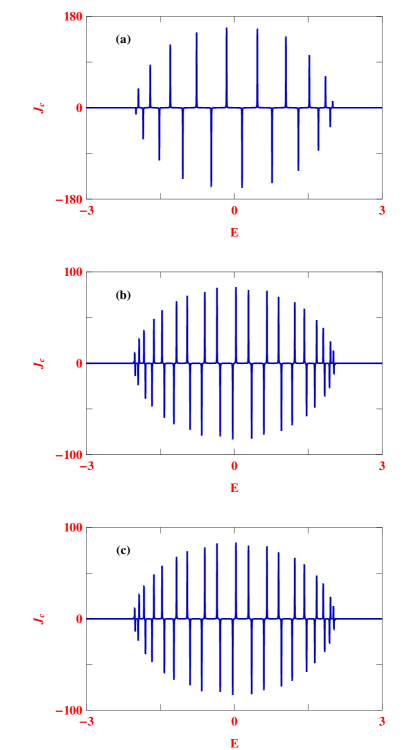
Figure 2: (Color online). Persistent charge current density as a function of energy for a $20$-site ordered ring setting $\phi=\phi_{0}/4$, where (a) $\alpha=\beta=0$, (b) $\alpha=0.2$ and $\beta=0$, and (c) $\alpha=0$ and $\beta=0.2$.

values of Rashba and Dresselhaus spin-orbit fields. The results are computed for a $20$-site impurity-free mesoscopic ring when the AB flux $\phi$ is set at $\phi_{0}/4$. For a better viewing of distinct peaks in the density spectrum here we display the results for such a small size ring. Several interesting patterns are obtained those can be analyzed as follows. From the spectra it is observed that the charge current density exhibits sharp peaks and dips for some particular energy values, while it drops to zero for other energies. All these peaks and dips are associated with the energy eigenvalues of the ring.

For the particular case when the ring is free from any kind of SO interaction and subjected to a non-zero magnetic flux, apart from integer or half-integer multiples of the elementary flux-quantum, the energy levels are two-fold degenerate which results in total $20$ peaks and dips in the current density spectrum (see Fig. 2(a)). It is quite interesting to note that the peaks and dips appear alternately throughout the band spectrum which essentially leads to an important conclusion that successive energy levels carry currents in opposite directions. This behavior suggests the vanishing net current for the complete band filling.

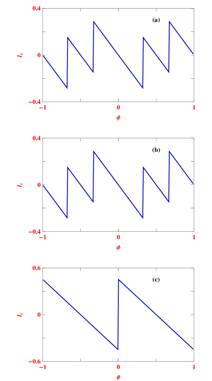
Figure 3: (Color online). Persistent charge current as a function of flux $\phi$ for a $60$-site ordered ring, where (a) $\alpha=0.3$ and $\beta=0$, (b) $\alpha=0$ and $\beta=0.3$, and (c) $\alpha=\beta=0.3$. The chemical potential $\mu$ is fixed at $0$.

Furthermore, one can also utilize this charge current density spectrum to predict the nature of extendedness of different energy levels by superimposing the average density of states (ADOS) on it. A non-zero contribution, viz, a peak or a dip, to the charge current will be obtained from the conducting states, while it becomes zero for the localized ones. This is another way of estimating the localization phenomenon in addition to the conventional methodologies maiti11 ; maiti12 ; maiti13 .

The charge current density spectrum gets significantly modified when we include SO coupling in this AB ring. The results are shown in Figs. 2(b) and (c), where in (b) we set a finite value of RSOI strength keeping the strength of DSOI as zero, while in (c) these parameter values get interchanged. It shows that the total number of peaks in the current density profiles, Figs. 2(b) and (c), associated with energy levels of the ring becomes exactly twice compared to the interacting free mesoscopic ring, viz., $\alpha=\beta=0$ (see Fig. 2(a)). This is because of the complete removal of degenerate energy eigenstates of the AB ring subjected to SO interaction. One more important property is also observed from these spectra (Figs. 2(b) and (c)) that the magnitude and sign of persistent charge current density $J_{c}$ for any energy window when the AB ring is subjected to RSOI only (Fig. 2(b)) are exactly identical to the ring described with only DSOI (Fig. 2(c)). Thus, it should be emphasized that the phase reversal in charge current density does not take place by interchanging the role played by $\alpha$ and $\beta$ into the Hamiltonian Eq. 1. This phenomenon can be implemented from the following analytical prescription.

The Rashba and Dresselhaus SO interaction terms, called as, $H_{\mbox{\tiny RSOI}}$ and $H_{\mbox{\tiny DSOI}}$ in the TB Hamiltonian Eq. 1 can be transformed into each other through a simple relation: $U^{{\dagger}}H_{\mbox{\tiny RSOI}}U$ = $H_{\mbox{\tiny DSOI}}$. Here, $U$ = $\left(\mbox{\boldmath$\sigma$}_{x}+\mbox{\boldmath$\sigma$}_{y}\right)/\sqrt{2}$ is the unitary matrix. Thus, any energy eigenstate $|\mathcal{M}^{\prime}\rangle$ of the transformed Hamiltonian $H_{\mbox{\tiny DSOI}}$ can be demonstrated in terms of the eigenstate $|\mathcal{M}\rangle$ of the Hamiltonian $H_{\mbox{\tiny RSOI}}$ through the relation $|\mathcal{M}^{\prime}\rangle$=$\mbox{\boldmath$U$}|\mathcal{M}\rangle$. This transformation leads to the charge current for the ring with only Dresselhaus SO coupling as,

$$J_{c}^{m}|_{\mbox{\tiny DSOI}} = \langle\mathcal{M}^{\prime}|\mbox{\boldmath$J$}_{c}|\mathcal{M}^{\prime}\rangle$$ (6)

$$= \langle\mathcal{M}|\mbox{\boldmath$U$}^{\dagger}\mbox{\boldmath$J$}_{c}\mbox{\boldmath$U$}|\mathcal{M}\rangle$$

$$= \langle\mathcal{M}|\mbox{\boldmath$U$}^{\dagger}\frac{e}{N}\mbox{\boldmath$\dot{x}$}\mbox{\boldmath$U$}|\mathcal{M}\rangle$$

$$= \langle\mathcal{M}|\frac{e}{N}\mbox{\boldmath$\dot{x}$}|\mathcal{M}\rangle$$

$$= J_{c}^{m}|_{\mbox{\tiny RSOI}}.$$

The above expression clearly establishes the reason for not affecting the sign and magnitude of charge current density upon the exchange of the role played by RSOI and DSOI.

Once the charge current density, $J_{c}(E)$, is evaluated using the relation presented in Eq. 3, the net persistent charge current $I_{c}$ in the ring can be easily determined by integrating the density spectrum (see Eq. 2) up to a certain energy range depending on the electron filling. As illustrative example, in Fig. 3 we present the variation of persistent charge current as a function of magnetic flux $\phi$ for an ordered ring considering different values of the SO coupling strengths. Here we set $N=60$ and $\mu=0$. The effect of the Rashba SO coupling is examined in the spectrum Fig. 3(a), setting the Dresselhaus SO interaction to zero. It is observed that the persistent charge current exhibits kink-like structures together with phase reversals at several values of flux $\phi$, which are however in general not unusual even in the absence of any SO coupling. These are essentially due to the band crossing in energy spectra and are immensely sensitive to the filling factor $\mu$. Though we have computed charge currents for different band fillings through ample numerical calculations, here we present results for a particular electron filling, as a test example, to establish our Green’s function approach for the estimation of persistent current in a

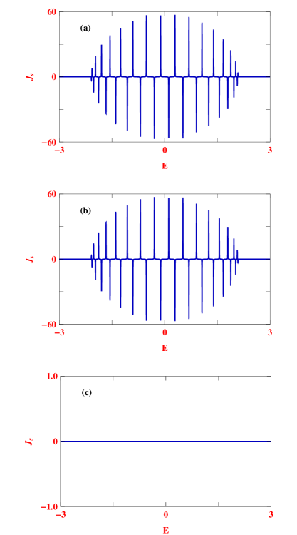
Figure 4: (Color online). Persistent spin current density as a function of energy for a $16$-site ordered ring, where (a) $\alpha=0.3$ and $\beta=0$, (b) $\alpha=0$ and $\beta=0.3$, and (c) $\alpha=\beta=0.3$. Here, we set $\phi=\phi_{0}/4$.

mesoscopic ring. In addition to the above issues it is also very important to point out that, for a particular value of the AB flux $\phi$ the current amplitude strongly depends on the chemical potential of the sample. An exhaustive analysis has already been given by Splettstoesser et al. spl in this line.

Figure 3(b) illustrates the situation in which the ring is described with DSOI only i.e., the other SO coupling term (RSOI) is set equal to zero. Since, the reversal of the roles governed by the variables $\alpha$ and $\beta$ into the TB Hamiltonian Eq. 1 does not anyway alter the physical picture of charge current density spectrum, the current-flux characteristics for the rings described with RSOI only (see Fig. 3(a)) become exactly identical to those with the rings in presence of DSOI only (see Fig. 3(b)). This phenomenon can also be justified from our analytical arguments presented in Eq. 6.

The combined outcome of both these two SO fields on persistent charge current is scrutinized in Fig. 3(c), where we specify $\alpha=\beta=0.3$. The other parameters are kept unchanged as taken in Figs. 3(a) and (b). In presence of both these two

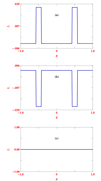
Figure 5: (Color online). Persistent spin current as a function of flux $\phi$ for a $100$-site ordered ring when the chemical potential $\mu$ is fixed at $0$, where (a) $\alpha=0.4$ and $\beta=0$, (b) $\alpha=0$ and $\beta=0.4$, and (c) $\alpha=\beta=0.4$.

interactions, the nature of persistent current for different values of $\phi$ changes appreciably compared to the case when only one SO interaction is present. This is due to the fact that the inclusion of both these two SO fields reforms the electronic band structure of the ring and thus strongly affects the pattern of the circulating current. In short, it can be emphasized that, charge current is distinctly sensitive to the SO coupling strength and magnetic flux threaded by the ring. All these currents vary repeatedly bearing $\phi_{0}$ ($=1$, in our choice of units where $c=e=h=1$) flux-quantum periodicity.

Now, we extend our discussion on persistent spin current in SO interaction induced impurity-free mesoscopic rings, where currents are computed from the Green’s function formalism. Before addressing these results, we first analyze the behavior of persistent spin current density, determined from the relation given in Eq. 5, to make this communication a self contained study. In Fig. 4 the energy dependent spin current density spectra are presented for a $16$-site ordered ring considering $\phi=\phi_{0}/4$, where the upper, middle and lower panels correspond to the results for three different set of parameter values of $\alpha$ and $\beta$. Interestingly, we see that the spin current density in the ring described with only Dresselhaus SO coupling (see Fig. 4(b)) changes its sign keeping the magnitude unaltered compared to the ring with RSOI only (see Fig. 4(a)). This sign reversal behavior can be viewed as follows. Using the similar prescription presented in Eq. 6, the spin current for the ring described with only DSOI gets the form,

$$J_{s}^{m}|_{\mbox{\tiny DSOI}} = \langle\mathcal{M}^{\prime}|\mbox{\boldmath$J$}_{s}|\mathcal{M}^{\prime}\rangle$$ (7)

$$= \langle\mathcal{M}|\mbox{\boldmath$U$}^{\dagger}\mbox{\boldmath$J$}_{s}\mbox{\boldmath$U$}|\mathcal{M}\rangle$$

$$= \langle\mathcal{M}|\mbox{\boldmath$U$}^{\dagger}\frac{1}{2N}\left(\mbox{\boldmath$\sigma_{z}\dot{x}$}+\mbox{\boldmath$\dot{x}\sigma_{z}$}\right)\mbox{\boldmath$U$}|\mathcal{M}\rangle$$

$$= \langle\mathcal{M}|\frac{1}{2N}\left(-\mbox{\boldmath$\sigma_{z}\dot{x}$}-\mbox{\boldmath$\dot{x}\sigma_{z}$}\right)|\mathcal{M}\rangle$$

$$= -J_{s}^{m}|_{\mbox{\tiny RSOI}}.$$

This relation clearly describes the sign reversal of spin current density upon the interchange of the parameters $\alpha$ and $\beta$ into the Hamiltonian (Eq. 1) of the ring. From this analysis we can also justify the vanishing nature of persistent spin current density for the entire density spectrum (see Fig. 4(c)) when the Dresselhaus SO interaction strength becomes precisely identical to the strength of the Rashba term. This is an interesting observation and may lead to a possible route for estimating the strength of anyone of the SO fields provided the other one is known. A detailed analysis of it can be obtained from the following current-flux characteristics.

Similar to persistent charge current, we also compute net persistent spin current $I_{s}$ in the ring by integrating the spin current density $J_{s}(E)$ (see Eq. 4) over a finite energy range associated with the filling factor $\mu$. As representative example, in Fig. 5 we show the variation of persistent spin current as a function of AB flux $\phi$ for a $100$-site ordered ring when the chemical potential $\mu$ is set at zero. Figure 5(a) illustrates the situation in which the ring is described with RSOI only, while in Figure 5(b) the effect of Dresselhaus SO coupling on spin current is presented. From these spectra (Figs. 5(a) and (b)) we observe that, spin current in the ring characterized with DSOI only alters its sign keeping the magnitude unchanged compared to the ring with Rashba term only, which is however exactly what we expect from the spin current density spectra shown in Fig. 4, since current is computed by integrating the density function $J_{s}$. The usual phase reversals at several values of AB flux $\phi$ associated with the band crossing in energy spectra together with $\phi_{0}$ flux-quantum periodicity are also noticed from these current-flux characteristics.

Certainly, whenever the strength of Dresselhaus SO coupling becomes exactly identical to that of Rashba SO interaction, spin current becomes zero for the entire flux window. It is shown in Fig. 5(c), where we set $\alpha=\beta=0.4$. This vanishing nature of persistent spin current is

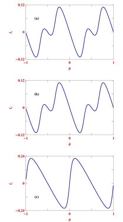
Figure 6: (Color online). Persistent charge current as a function of flux $\phi$ for a $60$-site ring in presence of disorder ($W=1$) for the same parameter values used in Fig. 3.

detected for any non-zero value of Rashba SO interaction provided it becomes equal to the Dresselhaus term, and also this behavior is independent of the band filling which we establish through our vast numerical calculations. This phenomenon, in principle, gives a possibility of estimating anyone of the SO fields if the other one is known. By means of an outside gate voltage one can control the Rashba SO coupling, and thus its strength can be determined. This suggests that, monitoring the RSOI in a mesoscopic ring we will get an absolute vanishing spin current when the strength of the Dresselhaus SO coupling becomes identical to that of the RSOI. Thus, from a realizable experimental measurement of persistent spin current one can evaluate the strength of Dresselhaus SO coupling. Additionally, it is also important to state that one may determine the strength of Rashba term employing this same mechanism provided the other term is known.

Up to now we have demonstrated the results for perfect rings. For more practical implications we now focus our attention on mesoscopic rings in presence of impurities. Impurities are introduced randomly in site potentials ($\epsilon_{n\uparrow}$ and $\epsilon_{n\downarrow}$) i.e.,

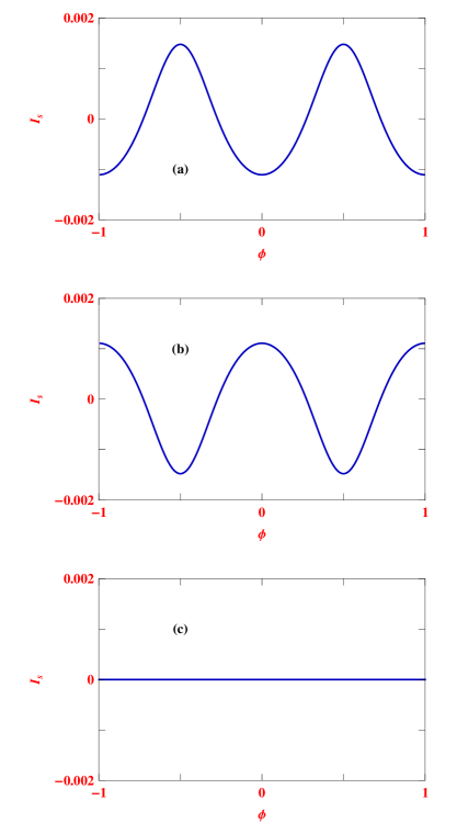
Figure 7: (Color online). Persistent spin current as a function of flux $\phi$ for a $100$-site ring in presence of disorder ($W=1$). The other model parameters are kept unchanged as used in Fig. 5.

diagonal disorder, through a ‘Box’ distribution function of width $W$, and the results averaged over $1000$ disorder configurations are presented. In Fig. 6 we present the results of persistent charge current for a disordered ring considering $W=1$ for different values of SO coupling strengths. Here we set $N=60$ and the results are computed for $\mu=0$, as a typical example. Several interesting features are obtained. Firstly, the current shows a continuous variation with flux $\phi$. This is essentially due to the fact that disorder makes a smooth variation of energy levels and eliminate band crossings those are mostly observed in impurity-free rings. The other important observation is that, in presence of impurities the current amplitude gets suppressed compared to the ordered case which can be clearly visible from the spectra plotted in Figs. 3 and 6. In presence of impurities the energy eigenstates are localized which results a reduction of persistent current, though this reduction is quite small compared to the ring without any SO interaction. In the absence of any SO coupling, disorder suppresses current amplitude almost to zero which is not unfamiliar in conventional disordered rings. But, with the inclusion of SO interaction current increases significantly and becomes quite proportionate to that of a perfect ring. A detailed analysis behind this mechanism has already been reported in our recent work maiti2 .

Finally, in Fig. 7 we present the results of persistent spin current in a mesoscopic ring to give a complete exposure of our Green’s function formalism for the evaluation of persistent current even in presence of impurities. Here we set $W=1$ and all the other parameters are kept unchanged as taken in Fig. 5. As usual the current varies continuously with flux $\phi$ exhibiting $\phi_{0}$ flux-quantum periodicity and it gets a reduced amplitude compared to the perfectly ordered ring. All the other properties i.e., the sign reversal upon the interchange of the role played by the parameters $\alpha$ and $\beta$ into the Hamiltonian Eq. 1 and the vanishing nature of spin current when the RSOI becomes equal to DSOI, remain exactly valid in the presence of impurities.

IV Summary and outlook

In the present work, we have proposed a new approach based on Green’s function formalism within a tight-binding framework to evaluate precisely the persistent charge and spin currents in spin-orbit interaction induced AB rings. The essential results are summarized as follows.

As already pointed out that, the standard methodology to the determination of circulating charge and spin currents in isolated conducting loops is based on the evaluation of eigenvalues and eigenvectors of the system Hamiltonian, which is highly numerically unstable especially for large size rings. Not only that it is really very hard to generalize in presence of interaction with external baths, if any. The present approach, the so-called Green’s function technique, circumvents the need to determine eigenvalues and eigenvectors of the system, and in particular, this methodology should give us access to predict the magnetic properties of large conducting rings as well as molecular rings encountered in biopolymers. We strongly believe that the present analysis yields persistent currents a very high degree of accuracy and leads to consider interplay of AB flux and geometry in magneto-transport of conducting loops subjected to Rashba and Dresselhaus SO fields.

It is worth pointing out that, in the present work we mainly concentrate on the new technique for the determination of persistent charge and spin currents. With this technique, we have also provided one possible route of estimating the strength of anyone of the SO fields provided the other one is known. This can be done by measuring persistent spin current which vanishes completely when the DSOI becomes equal to the RSOI, and this vanishing effect is also observed even in presence of impurities. It essentially supports us to propose an experiment towards this direction.

Before we end, we would like to mention that though we have computed persistent charge and spin currents for different band fillings considering different size rings through extensive numerical calculations, but here we have presented our results for some typical parameter values to explain the physical phenomena computed from our theoretical framework. All these physical pictures will be absolutely invariant for other parameter values also and thus demands the robustness of this new technique. In a forthcoming paper, we will provide the way of determining persistent charge and spin currents using this Green’s function technique considering the effect of electron-electron interaction.

Appendix A Green’s function approach for persistent charge current density when the ring is free from SO interactions

First, we consider the model quantum ring, presented in Fig. 1, and establish persistent charge current density in terms of Green’s function setting $\alpha=\beta=0$. Under this condition, TB Hamiltonian of the ring with site energy $\epsilon_{n}$ and nearest-neighbor hopping interaction $t$ becomes,

$$H = \sum_{n}\epsilon_{n}\,c_{n}^{\dagger}c_{n}+\sum_{n}\left(c_{n+1}^{\dagger}\,t\,c_{n}e^{i\theta}+c_{n}^{\dagger}\,t\,c_{n+1}e^{-i\theta}\right).$$

In terms of the velocity operator $\dot{x}$ the charge current operator $J_{c}$ can be written as,

$$\mbox{\boldmath$J_{c}$}=\frac{1}{N}e\mbox{\boldmath${\dot{x}}$}=\frac{2\pi ie}{Nh}\left[\mbox{\boldmath${H}$},\mbox{\boldmath${x}$}\right],$$ (9)

where, ${x}$=$\sum\limits_{n}c_{n}^{\dagger}\,n\,c_{n}$ is the position operator. Substituting $H$ and $x$ in Eq. 9 and doing a quite long but straightforward calculation we eventually reach to the expression,

$$\mbox{\boldmath$J_{c}$}=\frac{2\pi ie}{Nh}\sum_{n}\left(c_{n}^{\dagger}\,t\,c_{n+1}e^{-i\theta}-c_{n+1}^{\dagger}\,t\,c_{n}e^{i\theta}\right),$$ (10)

and, for a particular energy eigenstate $|\mathcal{M}\rangle=\sum\limits_{p}a_{p}^{m}|p\rangle$, it leads to the persistent charge current:

$$J_{c}^{m} = \langle\mathcal{M}|\mbox{\boldmath$J_{c}$}|\mathcal{M}\rangle$$ (11)

$$= \frac{2\pi iet}{Nh}\sum_{n}\left(a_{n}^{m\,*}a_{n+1}^{m}e^{-i\theta}-a_{n+1}^{m\,*}a_{n}^{m}e^{i\theta}\right),$$

where, $|p\rangle$’s are the Wannier states and $a_{p}^{m}$’s (the superscript $m$ is used for the eigenstate $|\mathcal{M}\rangle$) are the corresponding coefficients. Utilizing this relation one can determine persistent charge currents for discrete energy levels, and therefore, at absolute zero temperature net current carried by the ring will be the sum of individual contributions of some specific energy levels associated with the electron filling. This approach requires direct evaluation of energy eigenvalues and eigenstates, like other conventional methods available in literature gefen ; spl ; maiti2 ; bouz ; giam ; yu ; maiti8 ; maiti10 . To avoid it, we reframe the above current expression (Eq. 11) in terms of Green’s functions introducing the concept of current density, instead of defining conventional currents for individual energy levels. The prescription is as follows.

We start with the Green’s function of the ring $\mbox{\boldmath$G$}^{r}=\left(\mbox{\boldmath$E$}-\mbox{\boldmath$H$}+i\eta\mbox{\boldmath$I$}\right)^{-1}$. It leads to

$$\mbox{\boldmath$G$}_{ij}^{r} = \langle i|\mbox{\boldmath$G$}^{r}|j\rangle$$ (12)

$$= \sum_{m}\langle i|\mbox{\boldmath$G$}^{r}|\mathcal{M}\rangle\langle\mathcal{M}|j\rangle$$

$$= \sum_{m}\langle i|\left(\mbox{\boldmath$E$}-\mbox{\boldmath$H$}+i\eta\mbox{\boldmath$I$}\right)^{-1}|\mathcal{M}\rangle\langle\mathcal{M}|j\rangle$$

$$= \sum_{m}\frac{\langle i|\mathcal{M}\rangle\langle\mathcal{M}|j\rangle}{E-\mathcal{E}_{m}+i\eta}$$

$$= \sum_{m}\frac{a_{i}^{m}\,a_{j}^{m\,*}}{E-\mathcal{E}_{m}+i\eta},$$

where, $|\mathcal{M}\rangle$’s are the eigenstates of $H$ satisfying the relation $\sum\limits_{m}|\mathcal{M}\rangle\langle\mathcal{M}|=\mbox{\boldmath$I$}$ and $\mathcal{E}_{m}$ is the eigenvalue for the state $|\mathcal{M}\rangle$. $a_{i}^{m}$’s are the coefficients as described earlier. In a similar way we find,

$$\mbox{\boldmath$G$}_{ij}^{a}=\sum_{m}\frac{a_{i}^{m}\,a_{j}^{m\,*}}{E-\mathcal{E}_{m}-i\eta}.$$ (13)

Equations 12 and 13 yield,

$$\mbox{\boldmath$G$}_{ij}^{r}-\mbox{\boldmath$G$}_{ij}^{a} = \sum_{m}a_{i}^{m}a_{j}^{m\,*}\left(\frac{1}{E-\mathcal{E}_{m}+i\eta}-\frac{1}{E-\mathcal{E}_{m}-i\eta}\right)$$ (14)

$$= \sum_{m}a_{i}^{m}a_{j}^{m\,*}\left(\frac{-2i\eta}{(E-\mathcal{E}_{m})^{2}+\eta^{2}}\right)$$

$$= \sum_{m}a_{i}^{m}a_{j}^{m\,*}(-2i\eta)\,\frac{\pi}{\eta}\,\delta(E-\mathcal{E}_{m})$$

$$\hskip 56.9055pt(\mbox{in the limit}~{}\eta\rightarrow 0^{+})$$

$$= -2i\pi\sum_{m}a_{i}^{m}a_{j}^{m\,*}\,\delta(E-\mathcal{E}_{m}).$$

Interchange of the indices $i$ and $j$ in Eq. 14 generates,

$$\mbox{\boldmath$G$}_{ji}^{r}-\mbox{\boldmath$G$}_{ji}^{a}=-2i\pi\sum_{m}a_{i}^{m\,*}a_{j}^{m}\,\delta(E-\mathcal{E}_{m}).$$ (15)

It is clearly seen from Eqs. 14 and 15 that the non-zero contributions will only appear when the energy $E$ becomes equal to the discrete energy eigenvalues $\mathcal{E}_{m}$. This immediately allows us to express charge current density combining Eqs. 11, 14 and 15 as,

$$J_{c}(E) = -\frac{et}{Nh}\sum_{n}\left\{\left(\mbox{\boldmath$G$}_{n+1,n}^{r}-\mbox{\boldmath$G$}_{n+1,n}^{a}\right)e^{-i\theta}\right.$$ (16)

$$\left.-\left(\mbox{\boldmath$G$}_{n,n+1}^{r}-\mbox{\boldmath$G$}_{n,n+1}^{a}\right)e^{i\theta}\right\}.$$

This is the desired expression of charge current density in terms of Green’s functions when the ring is free from SO interactions.

Appendix B Green’s function approach for persistent charge current density when the ring is subjected to Rashba and Dresselhaus SO interactions

Next, we consider the ring with both Rashba and Dresselhaus SO interactions. The TB Hamiltonian of the ring presented in Eq. 1 can be expressed in a similar look of Eq. LABEL:ap1 like,

$$\mbox{\boldmath$H$}_{R} = \sum_{n}\mbox{\boldmath$c_{n}^{\dagger}\epsilon_{n}c_{n}$}+\sum_{n}\left(\mbox{\boldmath$c_{n+1}^{\dagger}t_{\varphi}^{n,n+1}c_{n}$}e^{i\theta}\right.$$ (17)

$$\left.+\,\mbox{\boldmath$c_{n}^{\dagger}t_{\varphi}^{\dagger n,n+1}c_{n+1}$}e^{-i\theta}\right),$$

where, different elements of the matrix $t_{\varphi}^{n,n+1}$ are:

$$\mbox{\boldmath$t_{\varphi}^{n,n+1}$}_{1,1} = t$$

$$\mbox{\boldmath$t_{\varphi}^{n,n+1}$}_{1,2} = -i\,\alpha\,e^{-i\varphi_{n,n+1}}+\beta\,e^{i\varphi_{n,n+1}}$$

$$\mbox{\boldmath$t_{\varphi}^{n,n+1}$}_{2,1} = -i\,\alpha\,e^{i\varphi_{n,n+1}}-\beta\,e^{-i\varphi_{n,n+1}}$$

$$\mbox{\boldmath$t_{\varphi}^{n,n+1}$}_{2,2} = t.$$

This TB Hamiltonian leads to the charge current operator following the prescription given in Eq. 9 and considering $\mbox{\boldmath$x$}=\sum\limits_{n}\mbox{\boldmath$c_{n}^{\dagger}nc_{n}$}$ in the form:

$$J_{c} = \frac{2\pi ie}{N}\sum_{n}\left(\mbox{\boldmath$c_{n}^{\dagger}t_{\varphi}^{\dagger\,n,n+1}$}\mbox{\boldmath$c_{n+1}$}\,e^{-i\theta}\right.$$ (18)

$$\left.-\,\mbox{\boldmath$c_{n+1}^{\dagger}t_{\varphi}^{n,n+1}$}\mbox{\boldmath$c_{n}$}\,e^{i\theta}\right).$$

Hence, for a particular eigenstate $|\mathcal{M}\rangle$ ($=\sum\limits_{p}a_{p,\uparrow}^{m}|p\uparrow\rangle+a_{p,\downarrow}^{m}|p\downarrow\rangle$) the charge current is written as,

$$J_{c}^{m} = \frac{2\pi ie}{N}\sum_{n}\left(\mbox{\boldmath$a_{n}^{m\,*}\,t_{\varphi}^{\dagger\,n,n+1}$}\,\mbox{\boldmath$a_{n+1}^{m}$}\,e^{-i\theta}\right.$$ (19)

$$\left.-\,\mbox{\boldmath$a_{n+1}^{m\,*}\,t_{\varphi}^{n,n+1}$}\,\mbox{\boldmath$a_{n}^{m}$}\,e^{i\theta}\right),$$

where, $a_{n}^{m}$=$\left(\begin{array}[]{c}a_{n\uparrow}^{m}\vspace{2mm}\\ a_{n\downarrow}^{m}\end{array}\right)$ and $a_{n}^{m\,*}$=$\left(\begin{array}[]{cc}a_{n\uparrow}^{m\,*}&a_{n\downarrow}^{m\,*}\end{array}\right)$. After simplification Eq. 19 yields,

$$J_{c}^{m} = \frac{2\pi ie}{N}\sum_{n}\left\{t\,a_{n,\uparrow}^{m\,*}a_{n+1,\uparrow}^{m}\,e^{-i\theta}-t\,a_{n+1,\uparrow}^{m\,*}a_{n,\uparrow}^{m}\,e^{i\theta}\right\}$$ (20)

$$+ \frac{2\pi ie}{N}\sum_{n}\left\{t\,a_{n,\downarrow}^{m\,*}a_{n+1,\downarrow}^{m}\,e^{-i\theta}-t\,a_{n+1,\downarrow}^{m\,*}a_{n,\downarrow}^{m}\,e^{i\theta}\right\}$$

$$+ \frac{2\pi ie}{N}\sum_{n}\left\{\left(i\alpha e^{-i\varphi_{n,n+1}}-\beta e^{i\varphi_{n,n+1}}\right)\right.$$

$$\left.\hskip 56.9055pt\times\,a_{n,\uparrow}^{m\,*}a_{n+1,\downarrow}^{m}e^{-i\theta}\right.$$

$$+ \left.\left(i\alpha e^{i\varphi_{n,n+1}}+\beta e^{-i\varphi_{n,n+1}}\right)a_{n+1,\downarrow}^{m\,*}a_{n,\uparrow}^{m}e^{i\theta}\right\}$$

$$+ \frac{2\pi ie}{N}\sum_{n}\left\{\left(i\alpha e^{i\varphi_{n,n+1}}+\beta e^{-i\varphi_{n,n+1}}\right)\right.$$

$$\left.\hskip 56.9055pt\times\,a_{n,\downarrow}^{m\,*}a_{n+1,\uparrow}^{m}e^{-i\theta}\right.$$

$$+ \left.\left(i\alpha e^{-i\varphi_{n,n+1}}-\beta e^{i\varphi_{n,n+1}}\right)a_{n+1,\uparrow}^{m\,*}a_{n,\downarrow}^{m}e^{i\theta}\right\}.$$

With this explicit expression (Eq. 20) and following the above prescription described in Appendix A, we eventually get the final result Eq. 3 for persistent charge current density in presence of SO fields.

Appendix C Green’s function approach for polarized spin current density when the ring is subjected to Rashba and Dresselhaus SO interactions

Finally, we derive the expression of persistent spin current density in presence of SO fields. To do this we begin with the spin current operator,

$$\mbox{\boldmath$J_{s}$}=\frac{1}{2N}\left(\mbox{\boldmath${\sigma}$}\mbox{\boldmath${\dot{x}}$}+\mbox{\boldmath${\dot{x}}$}\mbox{\boldmath${\sigma}$}\right),$$ (21)

where, $\mbox{\boldmath${\sigma}$}=\{\mbox{\boldmath${\sigma_{x}}$},\mbox{\boldmath${\sigma_{y}}$},\mbox{\boldmath${\sigma_{z}}$}\}$. Along the spin quantized direction ($+Z$) this equation (Eq. 21) reduces to,

$$\mbox{\boldmath$J_{s}^{z}$}=\frac{1}{2N}\left(\mbox{\boldmath${\sigma_{z}}$}\mbox{\boldmath${\dot{x}}$}+\mbox{\boldmath${\dot{x}}$}\mbox{\boldmath${\sigma_{z}}$}\right).$$ (22)

Now, using the TB form given in Eq. 17 and following the same prescription of Eq. LABEL:ap1 we can express Eq. 22 doing a straightforward and somewhat lengthy algebra as,

$$J_{s}^{z} = \frac{i\pi}{N}\sum_{n}\left(\mbox{\boldmath$c_{n}^{\dagger}\sigma_{z}t_{\varphi}^{\dagger\,n,n+1}$}\mbox{\boldmath$c_{n+1}$}\,e^{-i\theta}\right.$$ (23)

$$- \left.\mbox{\boldmath$c_{n+1}^{\dagger}\sigma_{z}t_{\varphi}^{n,n+1}$}\mbox{\boldmath$c_{n}$}\,e^{i\theta}\right)$$

$$+ \frac{i\pi}{N}\sum_{n}\left(\mbox{\boldmath$c_{n}^{\dagger}t_{\varphi}^{\dagger\,n,n+1}\sigma_{z}$}\mbox{\boldmath$c_{n+1}$}\,e^{-i\theta}\right.$$

$$- \left.\mbox{\boldmath$c_{n+1}^{\dagger}t_{\varphi}^{n,n+1}\sigma_{z}$}\mbox{\boldmath$c_{n}$}\,e^{i\theta}\right).$$

This spin current operator under the operation $\langle\mathcal{M}|\mbox{\boldmath$J_{s}^{z}$}|\mathcal{M}\rangle$ yields persistent spin current for a particular eigenstate $|\mathcal{M}\rangle$,

$$J_{s}^{z,m} = \frac{2\pi it}{N}\sum_{n}\left\{a_{n,\uparrow}^{m\,*}a_{n+1,\uparrow}^{m}\,e^{-i\theta}-a_{n+1,\uparrow}^{m\,*}a_{n,\uparrow}^{m}\,e^{i\theta}\right\}$$

$$- \frac{2\pi it}{N}\sum_{n}\left\{a_{n,\downarrow}^{m\,*}a_{n+1,\downarrow}^{m}\,e^{-i\theta}-a_{n+1,\downarrow}^{m\,*}a_{n,\downarrow}^{m}\,e^{i\theta}\right\}.$$

This relation leads to the final result Eq. 5 following the approach given in Appendix A.

References

- (1) S. Datta, Electronic transport in mesoscopic systems, Cambridge University Press, Cambridge (1995).
- (2) Y. Imry, Introduction to mesoscopic physics, Oxford University Press, Oxford (1997).
- (3) S. Datta, Quantum transport: Atom to transistor, Cambridge University Press, Cambridge (2005).
- (4) N. Bayers and C. N. Yang, Phys. Rev. Lett. 7, 46 (1961).
- (5) M. Büttiker, Y. Imry, and R. Landauer, Phys. Lett. A 96, 365 (1983).
- (6) H. F. Cheung, Y. Gefen, E. K. Reidel, and W. H. Shih, Phys. Rev. B 37, 6050 (1988).
- (7) V. Ambegaokar and U. Eckern, Phys. Rev. Lett. 65, 381 (1990).
- (8) A. Schmid, Phys. Rev. Lett. 66, 80 (1991).
- (9) U. Eckern and A. Schmid, Europhys. Lett. 18, 457 (1992).
- (10) H. Bary-Soroker, O. Entin-Wohlman, and Y. Imry, Phys. Rev. B 82, 144202 (2010).
- (11) S. K. Maiti, J. Chowdhury and S. N. Karmakar, J. Phys.: Condens Matter 18, 5349 (2006).
- (12) S. K. Maiti, J. Chowdhury and S. N. Karmakar, Phys. Lett. A 332, 497 (2004).
- (13) S. K. Maiti and A. Chakrabarti, Phys. Rev. B 82, 184201 (2010).
- (14) P. Dutta, S. K. Maiti, and S. N. Karmakar, Phys. Lett. A 378, 1388 (2014).
- (15) S. K. Maiti, J. Chowdhury, and S. N. Karmakar, Solid State Commun. 135, 278 (2005).
- (16) S. K. Maiti, Phys. Status Solidi B 248, 1933 (2011).
- (17) S. K. Maiti, Int. J. Mod. Phys. B 21, 179 (2007).
- (18) S. K. Maiti, Quantum Matter 3, 413 (2014).
- (19) S. K. Maiti, J. Chowdhuri, and S. N. Karmakar, Synthetic Metals 155, 430 (2005).
- (20) L. P. Lévy, G. Dolan, J. Dunsmuir, and H. Bouchiat, Phys. Rev. Lett. 64, 2074 (1990).
- (21) E. M. Q. Jariwala, P. Mohanty, M. B. Ketchen, and R. A. Webb, Phys. Rev. Lett. 86, 1594 (2001).
- (22) N. O. Birge, Science 326, 244 (2009).
- (23) V. Chandrasekhar, R. A. Webb, M. J. Brady, M. B. Ketchen, W. J. Gallagher, and A. Kleinsasser, Phys. Rev. Lett. 67, 3578 (1991).
- (24) W. Rabaud, L. Saminadayar, D. Mailly, K. Hasselbach, A. Benoit, and B. Etienne, Phys. Rev. Lett. 86, 3124 (2001).
- (25) D. Mailly, C. Chapelier, and A. Benoit, Phys. Rev. Lett. 70, 2020 (1993).
- (26) H. Bluhm, N. C. Koshnick, J. A. Bert, M. E. Huber, and K. A. Moler, Phys. Rev. Lett. 102, 136802 (2009).
- (27) R. A. Smith and V. Ambegaokar, Europhys. Lett. 20, 161 (1992).
- (28) H. Bouchiat and G. Montambaux, J. Phys. (Paris) 60, 2695 (1989).
- (29) E. Gambetti-Césare, D. Weinmann, R. A. Jalabert, and Ph. Brune, Europhys. Lett. 60, 120 (2002).
- (30) Q.-F. Sun, X. C. Xie and J. Wang, Phys. Rev. Lett. 98, 196801 (2007).
- (31) V. Vlaminck and M. Bailleul, Science 322, 410 (2008).
- (32) K. Ando, S. Takahashi, K. Harii, K. Sasage, J. Ieda, S. Maekawa, and E. Saitoh, Phys. Rev. Lett. 101, 036601 (2008).
- (33) K. Ando, H. Nakayama, Y. Kajiwara, D. Kikuchi, K. Sasage, K. Uchida, K. Ikeda, and E. Saitoh, J. Appl. Phys. 105, 07C913 (2009).
- (34) Y. A. Bychkov and E. I. Rashba, JETP Lett. 39, 78 (1984).
- (35) G. Dresselhaus, Phys. Rev. 100, 580 (1955).
- (36) L. Meier, G. Salis, I. Shorubalko, E. Gini, S. Schon, and K. Ensslin, Nature Phys. 4, 77 (2008).
- (37) J. Premper, M. Trautmann, J. Henk, and P. Bruno, Phys. Rev. B 76, 073310 (2007).
- (38) R. Winkler, Spin-orbit coupling effects in two-dimensional electron and hole systems, Springer (2003).
- (39) J. S. Sheng and K. Chang, Phys. Rev. B 74, 235315 (2006).
- (40) J. Splettstoesser, M. Governale, and U. Zülicke, Phys. Rev. B 68, 165341 (2003).
- (41) D. Loss, P. Goldbart, and A. V. Balatsky, Phys. Rev. Lett. 65, 1655 (1990).
- (42) J. Nitta, T. Akazaki, H. Takayanagi, and T Enoki, Phys. Rev. Lett. 78, 1335 (1997).
- (43) C. Yin, B. Shen, Q. Zhang, F. Xu, N. Tang, L. Cen, X. Wang, Y. Chen, and J. Yu, Appl. Phys. Lett. 97, 181904 (2010).
- (44) M. Scheid, M. Kohda, Y. Kunihashi, K. Richter, and J. Nitta, Phys. Rev. Lett. 101, 266401 (2008).
- (45) M. Studer, M. P. Walser, S. Baer, H. Rusterholz, S. Schön, D. Schuh, W. Wegscheider, K. Ensslin, and G. Salis, Phys. Rev. B 82, 235320 (2010).
- (46) J. Schliemann, J. C. Egues, and D. Loss, Phys. Rev. Lett. 90, 146801 (2003).
- (47) B. A. Bernevig, J. Orenstein, and S.-C. Zhang, Phys. Rev. Lett. 97, 236601 (2006).
- (48) S. K. Maiti, S. Sil, and A. Chakrabarti, Phys. Lett. A 376, 2147 (2012).
- (49) S. K. Maiti, M. Dey, S. Sil, A. Chakrabarti, and S. N. Karmakar, Europhys. Lett. 95, 57008 (2011).
- (50) S. K. Maiti, J. Appl. Phys. 110, 064306 (2011).
- (51) G. Bouzerar, D. Poilblanc and G. Montambaux, Phys. Rev. B 49, 8258 (1994).
- (52) T. Giamarchi and B. S. Shastry, Phys. Rev. B 51, 10915 (1995).
- (53) N. Yu and M. Fowler, Phys. Rev. B 45, 11795 (1992).
- (54) S. K. Maiti, S. Saha, and S. N. Karmakar, Eur. Phys. J. B 79, 209 (2011).
- (55) S. K. Maiti, Solid State Commun. 150, 2212 (2010).
- (56) S. Saha, S. K. Maiti, and S. N. Karmakar, Eur. Phys. J. B 85, 283 (2012).
- (57) Q.-F. Sun and X. C. Xie, Phys. Rev. B 72, 245305 (2005).
- (58) S. Sil, S. K. Maiti, and A. Chakrabarti, Phys. Rev. Lett. 101, 076803 (2008).
- (59) S. Sil, S. K. Maiti, and A. Chakrabarti, Phys. Rev. B 78, 113103 (2008).
- (60) B. Pal, S. K. Maiti, and A. Chakrabarti, Europhys. Lett. 102, 17004 (2013).