Trees in random sparse graphs with a given degree sequence

Abstract.

Let $\mathbb{G}^{D}$ be the set of graphs $G(V,\,E)$ with $\left|V\right|=n$, and the degree sequence equal to $D=(d_{1},\,d_{2},\,\dots,\,d_{n})$. In addition, for $\frac{1}{2}<a<1$, we define the set of graphs with an almost given degree sequence $D$ as follows,

$$\mathbb{G}_{a}^{D}:=\cup\,\mathbb{G}^{\bar{D}},$$

where the union is over all degree sequences $\bar{D}$ such that, for $1\leq i\leq n$, we have $\left|d_{i}-\bar{d}_{i}\right|<d_{i}^{a}$.

Now, if we chose random graphs $\mathcal{G}_{\mathbf{g}}\left(D\right)$ and $\mathcal{G}_{\mathbf{a}}\left(D\right)$ uniformly out of the sets $\mathbb{G}^{D}$ and $\mathbb{G}_{a}^{D}$, respectively, what do they look like? This has been studied when $\mathcal{G}_{\mathbf{g}}\left(D\right)$ is a dense graph, i.e. $\left|E\right|=\Theta(n^{2})$, in the sense of graphons, or when $\mathcal{G}_{\mathbf{g}}\left(D\right)$ is very sparse, i.e. $d_{n}^{2}=o(\left|E\right|)$. In the case of sparse graphs with an almost given degree sequence, we investigate this question, and give the finite tree subgraph structure of $\mathcal{G}_{\mathbf{a}}\left(D\right)$ under some mild conditions. For the random graph $\mathcal{G}_{\mathbf{g}}\left(D\right)$ with a given degree sequence, we re-derive the finite tree structure in dense and very sparse cases to give a continuous picture.

Moreover, for a pair of vectors $\left(D_{1},D_{2}\right)\in\mathbb{Z}^{n_{1}}\times\mathbb{Z}^{n_{2}}$, we let $\mathcal{G}_{\mathbf{b}}\left(D_{1},D_{2}\right)$ be the random bipartite graph that is chosen uniformly out of the set $\mathbb{G}^{D_{1},D_{2}}$, where $\mathbb{G}^{D_{1},D_{2}}$ is the set of all bipartite graphs with the degree sequence $\left(D_{1},D_{2}\right)$. We are able to show the result for $\mathcal{G}_{\mathbf{b}}\left(D_{1},D_{2}\right)$ without any further conditions.

1. Introduction

1.1. Graphs with a given degree sequence.

Let $D=(d_{1},\,d_{2},\,\dots,\,d_{n})$ be a finite sequence of positive integers, such that $1\leq d_{1}\leq\cdots\leq d_{n}$, and $M:=\sum_{i=1}^{n}d_{i}$ is even. In addition, let $\mathbb{G}_{n}$ be the set of all simple graphs (undirected, with no loops or multiple edges) with $n$ vertices. For $G\in\mathbb{G}_{n}$, $\mathcal{V}(G)$ will be the set of its vertices indexed by $\{v_{1},v_{2},\ldots,v_{n}\}$ and $\mathcal{E}(G)$ is its set of edges $e:=\left\langle v_{i},v_{j}\right\rangle$. We say that $G$ is a graph with the given degree sequence $D$, if the degree of a vertex $v_{i}$ is $d_{i}$. It is evident that the total number of edges $|\mathcal{E}(G)|=\frac{1}{2}M$. We denote the set of all such simple graphs by $\mathbb{G}^{D}\subset\mathbb{G}_{n}$.

A random graph $\mathcal{G}_{\mathbf{g}}\left(D\right)$ with the given degree sequence $D$ is the one that is uniformly chosen from $\mathbb{G}^{D}$. Now, what does the random graph $\mathcal{G}_{\mathbf{g}}\left(D\right)$ look like? Researchers have studied this problem extensively, along with other properties of graphs with a given degree sequence. Before we list a couple of them here, we state some notations.

In this paper and for two real functions $f(n)$ and $g(n)$, the notations $g=\Theta(f)$, $g=O(f)$ and $g=o(f)$, as $n$ goes to infinity, mean that there exists a real number $C$ such that $\limsup_{n\rightarrow\infty}\frac{\left|f\right|}{\left|g\right|}+\frac{\left|g\right|}{\left|f\right|}\leq C$, $\limsup_{n\rightarrow\infty}\frac{\left|f\right|}{\left|g\right|}\leq C$ and $\lim_{n\rightarrow\infty}\frac{\left|f\right|}{\left|g\right|}=0$, respectively.

1.2. Dense graphs:

Dense graphs are those graphs $G\in\mathbb{G}_{n}$ that $\left|\mathcal{E}(G)\right|=\Theta\left(n^{2}\right).$ In [1], Barvinok and Hartigan studied the structure of dense graphs with a given degree sequence. They showed the relation between the maximum entropy function and the number of such graphs. Under mild conditions ($\delta$- tameness), they found the asymptotic behavior of the number of graphs with a given degree sequence $D$.

Although Barvinok and Hartigan provide an exact formula, it is difficult to touch it. There are also some other approaches to the counting problem which only work in certain regimes. In [19], Mckay and Wormald considered the case of graphs with nearly constant degree d, $\left|d_{i}-d\right|=O(n^{1/2})$, using a multidimensional saddle-point method. The enumeration of graphs with a given degree sequence may lead to finding the probabilities of subgraphs of random graph $\mathcal{G}_{\mathbf{g}}\left(D\right)$. Greenhill and Mckay studied that in [29] for various regimes. Also, see McKay [28] for a detailed survey of that subject.

Another approach toward graphs with a given degree sequence is through graph limits. Recently Lov́asz and Szegedy introduced, in [23], a notion of graph limits called graphons. This has been developed further by Borgs et al [8, 10, 9]. In regard to graphs with a given degree sequence, Chatterjee et al [6] showed that sequences of such graphs have graph limits, in the sense of graphons, if their degree sequences converge to a degree function which satisfies the Erdös-Gallai condition for graph limits.

1.3. Very sparse graphs:

Different regimes of very sparse graphs, $d_{max}^{2}=d_{n}^{2}=o(M)$, were studied a long time ago by Mckay, [27] and [26]. The condition allows us to comput the number of graphs via inclusion-exclusion and switching method. Mckay and Wormald came back to this problem in [30] with a less restrictive condition. Recently Gao et al [18] investigated the probability of subgraphs of a random graph with a given degree sequence in this regime. Look at [17] for more information about subgraphs of random graphs.

1.4. Bipartite graphs:

A bipartite graph is a graph with two set of vertices, where there are no edges with both ends in the same set. The adjacency matrix for a simple bipartite graph with a given degree sequence is a matrix with 0-1 entries with given row and column sums. Barvinok, in [2, 1], studied these matrices in the dense case. Barvinok and Hartigan generalized this in [4, 5] for matrices with non-negative integer entries. Like the case of usual graphs, they showed the relation of the number of bipartite graphs to entropy function. Look at [3] for a survey on the subject.

Canfield et al [11] derived a practical formula for matrices with 0-1 entries and nearly constant row and column sums. Canfield and Mckay, in [12], took a look at matrices with positive integer entries as well. Also, see [20] for similar results in sparse bipartite graphs.

1.5. A little bit of motivation:

Following the work of Lov́asz and Szegedy, many tried to extend the notion of graphons to the sparse graphs. Look at [7] for a survey of attempts to define a notion of limit in the sparse case. Here, we take another look at the subgraph counting metric. Let us recall the homomorphism density from page 2 of Lovász and Szegedy [23], which is

$$t\left(F,G\right):=\frac{\hom\left(F,G\right)}{\left|\mathcal{V}\left(G\right)\right|^{\left|\mathcal{V}\left(F\right)\right|}}.$$

In addition, graphs $G_{n}$ are said to be Cauchy in subgraph-counting metric if the sequence of numbers $t\left(F,G_{n}\right)$ are Cauchy for every finite graph $F$. So, we use a uniform normalization, i.e. $\left|\mathcal{V}\left(G\right)\right|^{\left|\mathcal{V}\left(F\right)\right|}$, for all embeddings of $F$ into $G$. However, we believe that the normalization should be local and depend on the embedding. We try to justify that throughout this paper.

Although we will not provide a metric for sparse graphs, we make a few observations in sparse random graphs with a given degree sequence. We adopt the method in [6] that compares the random graph $\mathcal{G}_{\mathbf{g}}\left(D\right)$ with a random graph $\widetilde{\mathcal{G}}\left(D\right)$, with independent Bernoulli random edges. By extending that work to sparse graphs, we obtain the correct normalization for counting the subgraph $F$, where $F$ is a tree. We leave the case the counting of subgraphs with loops open, since this problem has not been completely understood even in the case of random models with independent edges like Erdös–Ŕenyi graph. For more discussion, look at [22], [21], and [14]).

In this paper, we first introduce a modified version of graphs with the given degree sequence $D$, which we call graphs with an almost given degree sequence $D$. Then, under some mild conditions, we find the distribution of finite trees in this model. Second, we go back to our original problem and deal with random graph $\mathcal{G}_{\mathbf{g}}\left(D\right)$. In addition, we apply our method to dense, bipartite and very sparse, i.e. $d_{n}^{2}=o(\left|\mathcal{E}\left(G\right)\right|)$, random graphs.

Although we need some mild conditions in most of our theorems, we show that our results holds in full generality for bipartite random graphs. So we believe that the same is true for general non-bipartite graphs with a given degree sequence $D$. In the end, to the best of our knowledge, the method developed here is new and works for a wider range of graphs, from very sparse to dense graphs.

We begin the next section with some notation that is needed for the rest of the paper.

2. Main Results.

Let us start this section by stating a few notations. Throughout this section $c_{k}>0$ plays the role of a general constant that only depends on $k$. Now we provide the definitions of our independent model and ordered subgraphs.

2.1. Maximum entropy and the independent ensemble.

We let $\mathbb{P}^{D}$ be the set of all positive $x{}_{ij}$ satisfying

$$\sum_{j:\>j\neq i}^{n}x{}_{ij}=d_{i}.$$

Therefore, $\mathbb{P}^{D}$ is a polytope in $\mathbb{R}^{N}$, where $N$ is $\left(\begin{array}[]{c}\begin{array}[]{c}n\end{array}\\ 2\end{array}\right)$. Now, define the entropy function as follows,

(2.1) $$H_{1}(x):=\sum_{i<j}H(x_{ij}),\,\text{where }H(x)=-x\ln(x)-(1-x)\ln(1-x),$$

for $x=(x_{ij})\in\mathbb{R}^{N}$. We state a proposition that describes the necessary and sufficient condition for $\mathbb{P}^{D}$ to have a non-empty interior.

Proposition 2.1.

The polytope $\mathbb{P}^{D}$ has a non-empty interior if, and only if, the degree sequence satisfies the strict Erdös- Gallai conditions,

(2.2) $$\sum_{i=n-k+1}^{n}d_{i}<k(k-1)+\sum_{i=1}^{n-k}\min\left\{k,\,d_{i}\right\},\text{ for }1\leq k\leq n.$$

Remark 2.2.

If we turn the strict inequalities in (2.2) into “less than or equal to”, then we obtain the well-known Erdös- Gallai criterion Erdös and Gallai [16]. (See Mahadev and Peled [24] for extensive discussions.)

Now, if $\mathbb{P}^{D}$ has a non-empty interior, then the function $H_{1}(x)$ attains its maximum at a unique point, since it is strictly concave. Denote that maximum by $\widetilde{\mathbf{p}}=(\widetilde{p}{}_{ij})\in\mathbb{R}^{N}$, and define $\widetilde{\mathcal{G}}\left(D\right)$ as a random graph with independent Bernoulli random edges with parameters $\widetilde{p}{}_{ij}$. From the definition of the $\widetilde{\mathbf{p}}$ and for each $i\in[n]:=\left\{1,\cdots,n\right\}$, we see that the average degree of vertex $i$ in $\widetilde{\mathcal{G}}\left(D\right)$ is $d_{i}$. In other words,

(2.3) $$\sum_{j:\>j\neq i}^{n}E\left[\mathbf{1}_{\left\langle i,j\right\rangle}\left(\widetilde{\mathcal{G}}\left(D\right)\right)\right]=\sum_{j:\>j\neq i}^{n}\widetilde{p}{}_{ij}=d_{i},$$

where the indicator function $\mathbf{1}_{\left\langle i,j\right\rangle}\left(\widetilde{\mathcal{G}}\left(D\right)\right)$ is $1$ if $\left\langle i,j\right\rangle\in\widetilde{\mathcal{G}}\left(D\right)$ and $0$ otherwise. We also use “$\sim$” for parameters of $\widetilde{\mathcal{G}}\left(D\right)$, wherever possible.

Definition 2.3.

A vector of positive integers $D$ is a strict graphic sequence if the vector $D$ satisfies the strict Erdös- Gallai conditions (2.2).

Remark 2.4.

Definition 2.3 means that $\mathbb{P}^{D}$ has a non-empty interior, which in turn implies that the maximum entropy $\widetilde{\mathbf{p}}=(\widetilde{p}_{ij})$ exists.

2.2. Ordered trees and their B- function.

Let $\mathbb{T}^{k}$ be the set of all trees with a finite number $k$ of vertices. The famous Cayley’s Theorem states that there are $k^{k-2}$ of such trees, and for a proof of it, check [31]. For a tree $T\in\mathbb{T}^{k}$, we look at maps $s:\mathcal{V}(T)\to\mathcal{V}(G)$, which map the vertices of $T$ into distinct vertices of $\mathbb{G}_{n}$. There are $n(n-1)\cdots(n-k+1)$ of them, and let us call the set of all such maps $\mathbb{S}_{n}^{k}$, i.e.

$$\mathbb{S}_{n}^{k}=\{s:[k]\to[n]|\>s\text{ is }1-1\}.$$

In addition, an ordered tree is a pair $\left(s,T\right)\in\mathbb{S}_{n}^{k}\times\mathbb{T}^{k}$. For instance, if $k=2$, $\mathbb{S}_{n}^{2}\times\mathbb{T}^{2}$ is the set of directed edges on vertices of $\left[n\right]=\left\{1,\cdots,n\right\}$. (We drop the n in the index of $\mathbb{S}_{n}^{k}$, whenever the dependency on n is understood.)

Definition 2.5.

We let $\left(s,T\right)\in\mathbb{S}_{n}^{k}\times\mathbb{T}^{k}$ be an ordered tree. For each vertex $u\in\mathcal{V}(T)$, its degree in the tree $T$ is denoted by $b_{u}$. The B- function is defined as

(2.4) $$\psi\left(s,T,D\right)=\prod_{u\in V(T)}d_{s(u)}^{b_{u}-1}.$$

In addition, we denote $\psi(s,T,D\left(G\right))$ by $\psi(s,T,G)$, where $D\left(G\right)$ is the degree sequence of $G$.

Remark 2.6.

Let us consider a permutation $\pi$ on numbers $1$ through $k$. We observe that

$$\psi\left(s,T,D\right)=\psi\left(s\circ\pi^{-1},\pi\circ T,D\right).$$

Hence, we get $k!$ distinct ordered trees with the same B-function.

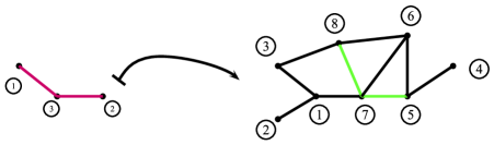
Figure 2.1. An ordered tree

The left graph is a labeled tree $T\in\mathbb{T}^{3}$ with 2 edges. The green graph on the right is the image of $T$ under a map $s$ that takes $1,3$ and $2$ to $8,7$ and $5$ respectively. Hence, the green graph is an ordered tree $\left(s,T\right)$ that sits inside a graph with degree sequence $D=\left(3,1,2,1,3,3,4,3\right).$ The corresponding B- function for $\left(s,T\right)$ is $d_{8}^{0}\cdot d_{7}^{2}\cdot d_{5}^{0}=4^{2}$.

2.3. Graphs with an almost given degree sequence:

We recall from the beginning of this paper that $D=\left(d_{1},\cdots,d_{n}\right)$, and $d_{1}\leq\cdots\leq d_{n}$, and $M=\sum_{i=1}^{n}d_{i}$. We let $S_{k}$ be the sum of biggest $d_{k}$ elements of $D$, or $S_{k}:=\sum d_{i}$, where the sum is over the set $\{n-d_{k},\cdots,n\}$. In addition, we define $\ell(D)$ as the maximum positive integer that $S_{\ell}\leq\frac{M}{2}$, i.e.

(2.5) $$\ell(D):=\max\left\{k\in[n]\Big{|}S_{k}\leq\frac{M}{2}\right\}.$$

Assumption 2.7.

Let us assume that, for some numbers $\epsilon>0$ and $\nu>0$,

1. the vector $D$ satisfies the strict Erdös- Gallai conditions (2.2).

2. the number $M=\sum_{i=1}^{n}d_{i}$ is even and $n^{1+\varepsilon}\leq M$.

3. and, for the function $\ell\left(D\right)$ as in (2.5),

   (2.6) $$\sqrt{\frac{n}{M}}\left(d_{n}-d_{\ell(D)}+1\right)<n^{-\nu}.$$

Definition 2.8.

In particular, we say that a vector $D$ is a strict graphic sequence of type $\left(\varepsilon,\,\nu\right)$, if it satisfies all of the above conditions, and is a strict graphic sequence of type $\varepsilon$, if $D$ only satisfies the first two conditions.

Remark 2.9.

Let us see a couple of examples to understand the term $d_{n}-d_{\ell(D)}$ and the above conditions. Suppose that $d_{n}^{2}<\frac{M}{2}$ (particularly, this is particularly the case when $d_{n}^{2}=o(M)$). Since $d_{n}$ is the maximum element of $D$, $S_{n}=\sum_{i=1}^{d_{n}}d_{n+1-i}$ is less than $d_{n}^{2}$, which means $\ell(D)$ is $n$. Hence, $d_{n}-d_{\ell(D)}=0$.

In another example, let $D$ be a sequence such that $2n^{\alpha}<d_{i}<n^{\beta}$, for $1\leq i\leq n$, and $\beta<\frac{1+\alpha}{2}$. Again, $S_{n}$ is less than $d_{n}^{2}$, so $S_{n}<n^{2\beta}<n^{1+\alpha}<M/2$. In both examples, we get an upper bound of $\sqrt{\frac{n}{M}}$ for Eq. (2.6). In particular, our sequence is of type $\left(\varepsilon,\,\nu\right)$ for any $\nu$ smaller than $\varepsilon/2$.

Let us pick a positive number $a$ such that $\frac{1}{2}<a<1$. Then, we define the set of graphs with an almost given degree sequence $D$ as follows,

$$\mathbb{G}_{a}^{D}:=\cup\,\mathbb{G}^{\bar{D}},$$

where the union is over all degree sequences $\bar{D}$ such that, for $1\leq i\leq n$, we have $\left|d_{i}-\bar{d}_{i}\right|<d_{i}^{a}$. Let a random graph with an almost given degree sequence $D$, $\mathcal{G}_{\mathbf{a}}\left(a,D\right)$, be a random graph that is uniformly chosen from the set $\mathbb{G}_{a}^{D}$.

Definition 2.10.

We define probabilities $\mathbf{p_{a}}\left(s,T\right)$ and $\mathbf{\widetilde{p}}\left(s,T\right)$ as

$$E\left[{\bf 1}_{s}(T,\mathcal{G}_{\mathbf{a}}\left(a,D\right))\right]\textit{ and }E\left[{\bf 1}_{s}(T,\widetilde{\mathcal{G}}\left(D\right))\right],$$

respectively, where

$${\bf 1}_{s}(T,G)=\prod_{\left\langle u_{1},u_{2}\right\rangle\in\mathcal{E}(T)}{\bf 1}_{\left\langle s(u_{1}),s(u_{2})\right\rangle\in\mathcal{E}(G)}(G),$$

$\mathcal{G}_{\mathbf{a}}\left(a,D\right)$ is as above, and $\widetilde{\mathcal{G}}\left(D\right)$ is defined in Section 2.1. We dropped the dependency of $\mathbf{p_{a}}\left(s,T\right)$ on $D$ and $a$, as well as the dependency of $\mathbf{\widetilde{p}}\left(s,T\right)$ on $D$ and $\mathbf{\widetilde{p}}$, the maximum entropy, for the simplicity of our notations.

Theorem 2.11.

Suppose that the vector $D$ is a strict graphic sequence of type $\left(\varepsilon,\,\nu\right)$ as in Definition 2.3. We define,

(2.7) $$L_{\mathbf{a}}\left(a,k,D\right):=\frac{1}{M}\sum_{\left(s,T\right)\in\mathbb{S}^{k}\times\mathbb{T}^{k}}\frac{1}{\psi\left(s,T,D\right)}\left|\mathbf{p_{a}}\left(s,T\right)-\mathbf{\widetilde{p}}\left(s,T\right)\right|,$$

where $\mathbb{T}^{k}$, $\mathbb{S}_{n}^{k}$ and $\psi\left(s,T,D\right)$ are defined in Section 2.2, and $\mathbf{p_{a}}\left(s,T\right)$ and $\mathbf{\widetilde{p}}\left(s,T\right)$ are the same as in Definition 2.10. If $\frac{1}{2}<a<\frac{\nu}{4}+\frac{1}{2}$, then

(2.8) $$L_{\mathbf{a}}\left(a,k,D\right)\leq c_{k}\cdot n^{a-\frac{\nu+1}{2}}=o(1).$$

Remark 2.12.

Recall from Remark 2.6 that $\psi\left(s,T,D\right)$ is invariant under the action of a permutation on the labels of an ordered tree $\left(s,T\right)$. In addition, the space $\mathbb{S}^{k}\times\mathbb{T}^{k}$ is a multi covering of

$$\mathcal{T}\left(k,n\right):=\cup_{T\in\mathbb{T}^{k}}\hom\left(T,K_{n}\right)$$

with $k!$ layers, where $K_{n}$ is the complete graph with $n$ vertices. Hence, if we take the sum over $\mathcal{T}\left(k,n\right)$ instead of $\mathbb{S}_{n}^{k}\times\mathbb{T}^{k}$, we get $\frac{L_{\mathbf{a}}\left(a,k,D\right)}{k!}$, which is still $o\left(1\right).$ Although the set $\mathbb{S}_{n}^{k}\times\mathbb{T}^{k}$ requires us to over-count objects, it also brings us symmetry and that makes it easier to deal with.

Remark 2.13.

For the examples in Remark 2.9, $n^{-\nu}$ is $\sqrt{\frac{n}{M}}$ and the bound in Eq. (2.8) becomes $O\left(\left(\frac{n}{M}\right)^{1/4}n^{a-\frac{1}{2}}\right)$. We believe that this is the correct bound on $L_{\mathbf{a}}\left(a,k,D\right)$, and also, we believe the last condition in Definition 2.3 is not necessary. We come back to this matter later in the proof section ( Conjecture 3.13 and Remark 3.14).

Remark 2.14.

The previous theorem is only stated for connected trees, however, the same result with the same proof is true for forests. The B-function, in that case, is the product of B-functions for each connected component. For example, for $k=2$ and forests with two connected components, Theorem 2.11 gives the joint probability distribution for two edges. Recall that $\mathbb{S}_{n}^{2}\times\mathbb{T}^{2}$ can be interpreted as the set of directed edges, and note that the B-function of each edge is $M$. Then, the corresponding result says

$$\frac{1}{M^{2}}\sum\left|p_{a,(ij)(kl)}-\widetilde{p}_{ij}\widetilde{p}_{kl}\right|=o(1),$$

where the sum is over all disjoint pairs of directed edges, $(i,j)$ and $(k,l)$, and

(2.9) $$p_{a,(ij)(kl)}:=E\left(\mathbf{1}_{\left\langle i,j\right\rangle\in\mathcal{E\left(\mathcal{G}_{\mathbf{a}}\right)}}\left(\mathcal{G}_{\mathbf{a}}\right)\mathbf{1}_{\left\langle k,l\right\rangle\in\mathcal{E\left(\mathcal{G}_{\mathbf{a}}\right)}}\left(\mathcal{G}_{\mathbf{a}}\right)\right),$$

for $\mathcal{G}_{\mathbf{a}}=\mathcal{G}_{\mathbf{a}}\left(a,D\right).$

Remark 2.15.

Let us explore the weights now. Suppose that all $\widetilde{p}_{ij}\simeq p$ are of the same order. Then it is not hard to see that $M\cdot\psi\left(s,T,D\right)$ is of order $\left(n^{2}\cdot p\right)\cdot\left(n\cdot p\right)^{k-2}\simeq n^{k}\mathbf{\widetilde{p}}\left(s,T\right)$, where $\left(s,T\right)\in\mathbb{S}^{k}\times\mathbb{T}^{k}$. Thus, $L_{\mathbf{a}}$ becomes

$$L_{\mathbf{a}}\left(a,k,D\right)\simeq\frac{1}{n^{k}}\sum_{\left(s,T\right)\in\mathbb{S}^{k}\times\mathbb{T}^{k}}\left|\frac{\mathbf{p_{a}}\left(s,T\right)}{\mathbf{\widetilde{p}}\left(s,T\right)}-1\right|.$$

In particular, if all degrees are $d$ ($d_{i}=d$, for every $i\in[n]$ and $1\leq d\leq n-1$), then symmetry implies that $p=\frac{d}{n-1}$, and that the independent model $\widetilde{\mathcal{G}}\left(D\right)$ is Erdös–Ŕenyi random graph $G(n,\frac{d}{n-1})$. The main point here is that the B- function gives the correct normalization.

Let us explore the statement of Theorem 2.11 for some small values of $k$. For $k=2$,

(2.10) $$L_{\mathbf{a}}\left(a,2,D\right)=\frac{1}{M}\sum_{1\leq i<j\leq n}\left|p_{a,(ij)}-\widetilde{p}{}_{ij}\right|\leq c_{k}\cdot n^{\frac{-\nu}{2}+a}=o(1),$$

where $p_{a,(ij)}:=E\left(\mathbf{1}_{\left\langle i,j\right\rangle\in\mathcal{E\left(\mathcal{G}_{\mathbf{a}}\right)}}\left(\mathcal{G}_{\mathbf{a}}\right)\right)$, and $\mathcal{G}_{\mathbf{a}}=\mathcal{G}_{\mathbf{a}}\left(a,D\right)$. Thus, the maximum entropy gives the edge probabilities in the random graph $\mathcal{G}_{a}$, i.e. $p_{a,(ij)}\sim\widetilde{p}{}_{ij}$.

For $k=3$, an ordered tree $\left(s,T\right)$ in $\mathbb{S}_{n}^{3}\times\mathbb{T}^{3}$ is a path of two edges, and its B- function is $d_{j}$, where $j$ is the middle vertex of the tree $s\left(T\right)$. Then, by Remark 2.12,

(2.11) $$\frac{L_{\mathbf{a}}\left(a,3,n\right)}{3!}=\sum_{j\in\left[n\right]}\sum_{\left\{i,k\right\}\subset\left[n\right]}\frac{1}{Md_{j}}\left|p_{a,(ij)(kl)}-\widetilde{p}{}_{ij}\widetilde{p}{}_{jk}\right|=o(1),$$

where $p_{a,(ij)(kl)}$ is defined in Eq. (2.9). Next, we make an observation about Eq. (2.7).

Theorem 2.16.

Suppose that $D$ is a strict graphic sequence of type $\varepsilon$ as in Definition 2.3. Then the sum of variables in Theorem 2.11 is nearly constant:

1. $$\frac{1}{M}\sum_{\left(s,T\right)\in\mathbb{S}^{k}\times\mathbb{T}^{k}}\frac{1}{\psi\left(s,T,D\right)}\mathbf{p_{a}}\left(s,T\right)=k^{k-2}+O\left(\left(\frac{n}{M}\right)^{1-a}\right),$$

2. and

   $$\frac{1}{M}\sum_{\left(s,T\right)\in\mathbb{S}^{k}\times\mathbb{T}^{k}}\frac{1}{\psi\left(s,T,D\right)}\mathbf{\widetilde{p}}\left(s,T\right)=k^{k-2}+O\left(\left(\frac{M}{n}\right)^{-\frac{1}{2}}\right),$$

3. moreover,

   (2.12) $$\frac{1}{M}\sum_{\left(s,T\right)\in\mathbb{S}^{k}\times\mathbb{T}^{k}}\frac{1}{\psi\left(s,T,D\right)}\left(\mathbf{p_{a}}\left(s,T\right)-\mathbf{\widetilde{p}}\left(s,T\right)\right)=O\left(\left(\frac{n}{M}\right)^{1-a}\right).$$

Remark 2.17.

The first part of Theorem 2.16 justifies the summation in the statement of Theorem 2.11, and shows that the weights do not overkill the summation. Moreover, Eq. (2.12) is Eq. (2.7) in Theorem 2.11 without the absolute sign. We will see later that the proof of the former equation is easier than the latter.

2.4. Graphs with a given degree sequence.

Recall that $\mathbb{G}^{D}$ is the set of all graphs with the degree sequence $D$. Let $\mathcal{G}_{\mathbf{g}}\left(D\right)$ be a random graph that is chosen uniformly out of the set $\mathbb{G}^{D}$. The random graph $\mathcal{G}_{\mathbf{g}}\left(D\right)$ is finer than the random graph $\mathcal{G}_{\mathbf{a}}\left(a,D\right)$ in the previous section. Because of a technical problem, we cannot provide the same result as in Theorem 2.11 in full generality. Therefore, we start with two conjectures. Then we continue with showing that the conjecture holds in various regimes, such as very sparse graphs, dense graphs, and bipartite graphs. In addition, we see the relevance of the existing results in the literature, in each case.

Conjecture 2.18.

Suppose that the vector $D$ is a strict graphic sequence of type $\varepsilon$ (2.3), and that the entropy function $H_{1}(x)$ takes its maximum at $\widetilde{\mathbf{p}}$, where $H_{1}(x)$ is defined in Eq. (2.1). Then, there exists a number $\eta>0$ independent of $n$ such that,

(2.13) $$e^{-\eta n\cdot\log(n)}\cdot e^{H_{1}(\widetilde{\mathbf{p}})}\leq\left|\mathbb{G}^{D}\right|\leq e^{H_{1}(\widetilde{\mathbf{p}})}.$$

We will see later that $P\left(\widetilde{\mathcal{G}}\left(D\right)\in\mathbb{G}^{D}\right)=\frac{\left|\mathbb{G}^{D}\right|}{e^{H_{1}(\widetilde{p})}}$. So, Eq. (2.13) reads

(2.14) $$e^{-\eta n\cdot\log(n)}\leq P\left(\widetilde{\mathcal{G}}\left(D\right)\in\mathbb{G}^{D}\right)=\frac{\left|\mathbb{G}^{D}\right|}{e^{H_{1}(\widetilde{\mathbf{p}})}}<1.$$

This proves the upper bound that is the easy part of the Conjecture 2.18. However, the lower bound that is crucial for our next Conjecture is open.

Conjecture 2.19.

Suppose that the vector $D$ is a strict graphic sequence of type $\varepsilon$. Let

$$\mathbf{p_{g}}\left(s,T\right)=E\left[{\bf 1}_{s}\left(T,\mathcal{G}_{\mathbf{g}}\left(D\right)\right)\right],$$

where ${\bf 1}_{s}\left(T,G\right)$ is defined in Eq. 2.10. Define,

(2.15) $$L_{\mathbf{g}}\left(k,D\right):=\frac{1}{M}\sum_{\left(s,T\right)\in\mathbb{S}_{n}^{k}\times\mathbb{T}^{k}}\frac{1}{\psi\left(s,T,D\right)}\left|\mathbf{p_{g}}\left(s,T\right)-\mathbf{\widetilde{p}}\left(s,T\right)\right|,$$

where $\mathbb{T}^{k}$, $\mathbb{S}_{n}^{k}$ and $\psi\left(s,T,D\right)$ are defined in Section 2.2, and $\mathbf{\widetilde{p}}\left(s,T\right)$ is as in Definition 2.10. Then we have,

$$L_{\mathbf{g}}\left(k,D\right)\leq c_{k}\cdot\sqrt{\frac{n\log(n)}{M}}.$$

Remark 2.20.

Conjecture 2.18 implies Conjecture 2.19, i.e.

$$e^{-\eta n\cdot\log(n)}\leq P\left(\widetilde{\mathcal{G}}\left(D\right)\in\mathbb{G}^{D}\right).$$

Thus, we have,

$$L_{\mathbf{g}}\left(k,D\right)\leq c_{k}\cdot\sqrt{\frac{n\log(n)}{M}}.$$

We will prove this in the Section 3.3.

2.5. Dense graphs with a given degree sequence:

In this section, we present why Theorem 2.11 and Conjecture 2.19 are true for dense graphs.

Definition 2.21.

For a positive number $c_{3}$ and numbers $c_{1},c_{2}\in(0,1)$, we say that a graph with degree sequence $D$ satisfies the dense Erdös - Gallai conditions of type $(c_{1},c_{2},c_{3})$, if

1. for every $i$

   $$c_{2}(n-1)\leq d_{i}\leq c_{1}(n-1),$$

2. and

   $$\frac{1}{n^{2}}\inf_{B\subseteq\{1,\cdots,n\},\left|B\right|\geq c_{2}n}\left\{\sum_{j\notin B}\min\left\{d_{j},\left|B\right|\right\}+\left|B\right|(\left|B\right|-1)-\sum_{i\in B}d_{i}\right\}\geq c_{3}.$$

Remark 2.22.

This definition implies that the vector $D$ is $\delta-tame$ in the sense that it was defined in [1], which means $\delta\leq\widetilde{p}_{ij}\leq 1-\delta$ for $\delta(c_{1},c_{2},c_{3})$, where $\widetilde{\mathbf{p}}=(\widetilde{p}_{ij})_{i,j}$ is the maximum entropy.

The next theorem is equivalent to the computations that appear in the last lines of the proof on page 34 of Theorem 1.1 in [6].

Theorem 2.23.

If the degree sequence $D$ satisfies the dense Erdös-Rényi condition (the preceding definition), then the Conjectures 2.18 and 2.19 hold. Therefore,

(2.16) $$L_{\mathbf{g}}\left(k,D\right)\leq c_{k}\cdot\left(n\log(n)\right)^{\frac{-1}{2}},$$

where $L_{\mathbf{g}}\left(k,D\right)$ is defined in Eq. (2.15). Moreover, for $\frac{1}{2}<a<\frac{1}{2}+\frac{1}{12}$, the Theorem 2.11 also holds, i.e.

(2.17) $$L_{\mathbf{a}}\left(a,k,D\right)\leq c_{k}\cdot n^{\frac{-3}{4}+a},$$

where $L_{\mathbf{a}}\left(a,k,D\right)$ is defined in Eq. (2.7).

2.6. Very sparse graphs with a given degree sequence:

Let us start this section with the very-sparseness definition.

Definition 2.24.

A graph with a degree sequence $D$ is called very sparse if $d_{n}^{2}=d_{\max}^{2}=o(M)$.

Now, we see the corresponding results to Theorem 2.11 and Conjecture 2.19 for very sparse random graphs. In addition, we see how our method is related to Mckay’s result.

Let us introduce new variables,

$$q_{ij}:=\frac{d_{i}d_{j}}{M+d_{i}d_{j}},\quad\text{where }1\leq i,j\leq n\text{ and }i\text{$\neq$}j.$$

Define $\mathcal{G}_{\mathbf{q}}\left(D\right)$ as a random graph with independent Bernoulli random edges with parameters $q{}_{ij}$. Let

(2.18) $$\mathbf{p_{q}}\left(s,T\right)=E\left[{\bf 1}_{s}\left(T,\mathcal{G}_{\mathbf{q}}\left(D\right)\right)\right],$$

where ${\bf 1}_{s}\left(T,G\right)$ is defined in Eq. 2.10. This random graph is an alternative to the random graph $\widetilde{\mathcal{G}}\left(D\right)$, which was constructed according to maximum entropy $\widetilde{\mathbf{p}}=(\widetilde{p}_{ij})_{i,j}$. The goal is to show that $\mathbf{p_{q}}\left(s,T\right)\simeq\mathbf{\widetilde{p}}\left(s,T\right)$, and in particular, $\widetilde{p}_{ij}\simeq q_{ij}$.

Theorem 2.25.

Suppose that $d_{n}^{2}=o(M)$, and that the vector $D$ is a strict graphic sequence of type $\varepsilon$. Let $L_{\mathbf{a}}\left(a,k,D\right)$ and $L_{\mathbf{g}}\left(k,D\right)$ be as in Eq. (2.7) and (2.15), and also define

(2.19) $$L_{\mathbf{q}}\left(k,D\right):=\frac{1}{M}\sum_{\left(s,T\right)\in\mathbb{S}_{n}^{k}\times\mathbb{T}^{k}}\frac{1}{\psi\left(s,T,D\right)}\left|\mathbf{p_{q}}\left(s,T\right)-\mathbf{\widetilde{p}}\left(s,T\right)\right|,$$

where we used the notations in Theorem 2.11, and $\mathbf{p_{q}}\left(s,T\right)$ is defined in Eq. (2.18). Then,

1. for random graph $\mathcal{G}_{\mathbf{a}}$, we have

   $$L_{\mathbf{a}}\left(a,k,D\right)\leq c_{k}\cdot\left(\frac{n}{M}\right)^{1/4}n^{a_{1}},$$

   where $a_{1}:=a-\frac{1}{2}$ is such that $\left(\frac{n}{M}\right)^{1/2}n^{3a_{1}}\ll 1$.

2. for random graph $\mathcal{G}_{\mathbf{g}}\left(D\right)$,

   $$L_{\mathbf{g}}\left(k,D\right)\leq c_{k}\cdot\left(\left(\frac{n}{M}\right)^{1/4}n^{a_{1}}+\frac{d_{n}^{2}}{M}\right).$$

3. moreover,

$$L_{\mathbf{q}}\left(k,D\right)\leq c_{k}\cdot\left(\left(\frac{n}{M}\right)^{1/4}n^{a_{1}}+\frac{d_{n}^{2}}{M}\right).$$

Remark.

The enumeration method used in Gao et al. [18] compares the random graphs $\mathcal{G}_{\mathbf{g}}\left(D\right)$, and $\mathcal{G}_{q}$. Whereas, through out this paper, we place the random graph $\mathcal{G}_{\mathbf{g}}\left(D\right)$ in comparison with the random graph $\widetilde{\mathcal{G}}\left(D\right)$, which comes from the maximum entropy. The previous theorem shows the relevance of the combinator method with respect to the general form by showing that $\widetilde{p}_{ij}\simeq q_{ij}$ (that is when $k=2$).

Remark.

Note that $\sum_{j=1}^{n}q_{ij}\neq d_{i}$, so the point $q=(q_{ij})$ is not on the polytope $\mathbb{P}^{D}$. However, the condition $d_{n}^{2}=o(M)$ demonstrates that this point is close to this polytope. In addition, the proof of the theorem depends on the combinatorial result of [27], so the condition $d_{n}^{2}=o(M)$ is necessary.

2.7. Bipartite graphs with an exact degree sequence:

In this section, we deal with bipartite graphs with a given degree sequence. Bipartite means that our graph has two vertex sets, namely set $1$ and $2$, and that there are no edges in between any two vertices of the same set. The advantage of the bipartite graphs is that Conjecture 2.18 holds, which is the subject of a paper of Barvinok [1]. They studied the number of 0-1 matrices with given row and column sums that are related to the problem of asymptotic enumeration for bipartite graphs, and the correspondence is given by the adjacency matrix of the graphs. This provides a way to state our results with no extra assumptions.

Let us start with a convention. We denote the parameters corresponding to each set of vertices by a number, either $1$ or $2$, in the subindex. Now, consider two integer vectors of $D_{i}=\left(d_{i,1},\cdots,d_{i,n_{i}}\right)$, for $i=1,2$, and $d_{i,1}\leq\cdots\leq d_{i,n_{i}}$. We say a bipartite graph has degree sequence $(D_{1},D_{2})$, if the degree sequence of the first vertex set is $D_{1}$ and the degree sequence of the second set is $D_{2}$. Let $n:=n_{1}+n_{2}$ be the total number of vertices, and denote the set of all bipartite graphs with a given degree sequence $(D_{1},D_{2})$ by $\mathbb{G}^{D_{1},D_{2}}$. The condition $\sum_{i}d_{1,i}=\sum_{j}d_{2,j}$ is enough to assure that $\mathbb{G}^{D_{1},D_{2}}$ is non-empty.

Since the nature of a bipartite graph does not allow it to have some of the edges or some of the trees as its subgraph, we should change our entropy function slightly and restrict our set of connected trees. Therefore, while the setup for bipartite graphs is a little bit different from previous cases, the ideas are the same. We state some definitions.

Definition 2.26.

Let us denote by $\mathcal{T}_{\mathbf{b}}\left(k,n\right)$ the ordered trees $\left(s,T\right)$ in $\mathbb{S}_{n}^{k}\times\mathbb{T}^{k}$ such that $s\left(T\right)$ does not have any edges with both ends in either set $1$ or set $2$.

Definition 2.27.

We let $\mathcal{G}_{\mathbf{b}}\left(D_{1},D_{2}\right)$ be the random bipartite graph with a given degree sequence $(D_{1},D_{2})$ that is uniformly chosen from the set $\mathbb{G}^{D_{1},D_{2}}$. Also, for $\left(s,T\right)\in\mathcal{T}_{b}^{k}$ , let

(2.20) $$\mathbf{p_{b}}\left(s,T\right)=E\left[{\bf 1}_{s}\left(T,\mathcal{G}_{\mathbf{b}}\left(D_{1},D_{2}\right)\right)\right],$$

where ${\bf 1}_{s}\left(T,G\right)$ is defined in 2.10. We do not show the dependency of $\mathbf{p_{b}}$ on $D_{1}$ and $D_{2}$ since it is understood.

For the maximum entropy we have the following new definition.

Definition 2.28.

Let us consider the polytope $\mathbb{P}^{D_{1},D_{2}}$ of matrices $X=(x_{ij})$ such that $\sum_{j=1}^{n_{2}}x_{ij}=d_{i,1}$ for $1\leq i\leq n_{1}$, and $\sum_{i=1}^{n_{1}}x_{ij}=d_{2,j}$ for $1\leq j\leq n_{2}$, and $0\leq x_{ij}\leq 1$ for all $i,\,j$. Also, define the entropy function for matrix $X=(x_{ij})$ as

$$H_{2}(x)=\sum_{i,\,j}H(x_{ij})\,\text{where }H(x)=-x\ln(x)-(1-x)\ln(1-x).$$

The entropy function $H_{2}(x)$ is strictly convex, hence, if the polytope $\mathbb{P}^{D_{1},D_{2}}$ has a non-empty interior, then the function $H_{2}(x)$ takes its maximum at some point $\widetilde{\mathbf{p}}\in\mathbb{P}^{D_{1},D_{2}}$.

Definition 2.29.

Consider the maximum entropy $\widetilde{\mathbf{p}}=(\widetilde{p}_{ij})_{i,j}$, where $1\leq i\leq n_{1}$, and $1\leq j\leq n_{2}$. This time, we define the random graph $\widetilde{\mathcal{G}}\left(D_{1},D_{2}\right)$ as a random graph that has independent Bernoulli random edges with probability $\widetilde{p}_{ij}$s, and let

(2.21) $$\mathbf{\widetilde{p}}\left(s,T\right)=E\left[{\bf 1}_{s}\left(T,\widetilde{\mathcal{G}}\left(D_{1},D_{2}\right)\right)\right].$$

Note that for the random graph $\widetilde{\mathcal{G}}\left(D_{1},D_{2}\right)$, there are no edges between the two vertices of set $1$ or two vertices of set $2$.

Theorem 2.30.

Suppose that the polytope $\mathbb{P}^{D_{1},D_{2}}$ has a non-empty interior, and define

(2.22) $$L_{\mathbf{b}}\left(k,D_{1},D_{2}\right):=\frac{1}{M}\sum_{\left(s,T\right)\in\mathcal{T}_{\mathbf{b}}\left(k,n\right)}\frac{1}{\psi\left(s,T,D\right)}\left|\mathbf{p_{b}}\left(s,T\right)-\mathbf{\widetilde{p}}\left(s,T\right)\right|,$$

where we used the notations in Theorem 2.11, and $\mathbf{p_{b}}\left(s,T\right)$ is defined in Eq. (2.20), and $D=\left(D_{1},D_{2}\right)$. Then, we obtain

$$L_{\mathbf{b}}\left(k,D_{1},D_{2}\right)\leq c_{k}\cdot\left(\frac{n\log(n)}{M}\right)^{\frac{1}{2}}.$$

Remark 2.31.

Note that we are able to prove the above result in almost the full generality, whereas in Conjecture 2.19, we needed an extra lower bound, which is discussed in Remark 2.20. Moreover, it is also possible to formulate the counter part of Theorem 2.11 for bipartite graphs and prove it without any extra condition. However, that is a repetition of the previous work and so we skip it.

Remark 2.32.

We observe that strict Erdös- Gallai conditions reduce to a much simpler equations in the case of bipartite graphs. However, dealing with that technicality is out of the scope of this paper, and we simply assume that $\mathbb{P}^{D_{1},D_{2}}$ has a non-empty interior.

2.8. Open questions

Here we list a couple of questions.

Question 1.:

Can we prove our results under fewer assumptions? In particular, is it possible to drop the last two parts of Definition 2.3, and only use the Erdös - Gallai conditions for our theorems? (see Conjecture 3.13)

Question 2.:

What can be said about triangle-counting in the sparse random graph $G$ with a given degree sequence $D$? How about other subgraphs?

Question 3.:

What is the correct way of counting the subgraphs? In the sense that, can we define a metric or a topology for the space of sparse graphs using the weighted subgraph counts?

Question 4.:

If the answer to the previous question is yes, are there any limiting objects under that metric?

Question 5.:

Is there any way to define a limiting object for graphs with a given degree sequence using the maximum entropy?

3. Proofs

The rest of the paper is organized as follows. In Section 3.1, we prove Theorems 2.16 and Theorem 2.11. For that, we use Theorem A.1 that is presented at the appendix with its proof. In Section 3.3, we see the proof of Remark 2.20. Then we prove Theorems 2.23, 2.25, and 2.30, in Sections 3.4, 3.5, and 3.6, respectively. We also use the notations in Sections 2.1 and 2.2 frequently.

3.1. Graph with an almost given degree sequence.

The aim of this section is to present the proof of Theorem 2.11, which will be completed in Subsection 3.1.2. Theorem 2.16 is required for this goal, so we start with a proof of that.

3.1.1. Proof of Theorem 2.16:

We see a few lemmas, and then the proof of Theorem 2.16.

Lemma 3.1.

(Upper bound). Let $T\in\mathbb{T}^{k}$ and $G\in\mathbb{G}^{D}$. If

$$F(T,G)=\sum_{s}\frac{1}{\psi(s,T,G)}\prod_{e=\left\langle u_{1},u_{2}\right\rangle\in\mathcal{E}(T)}{\bf 1}_{\left\langle s(u_{1}),s(u_{2})\right\rangle\in\mathcal{E}(G)}(G),$$

then $F(T,G)\leq M$.

Proof.

We prove it by induction on the size $k$ of the tree. We show that for any tree $T$ with $k$ vertices there is a tree $T^{\prime}$ with one vertex less such that

$$F(T,G)\leq F(T^{\prime},G),$$

for all $G$. Take any leaf $u_{1}$ of the tree, and suppose that $u_{1}$ is linked to $u_{2}$ by an edge. Note that $b_{u_{1}}=1$. Let $T_{k-1}$ be the tree obtained by deleting $u_{1}$ and the linking edge. If we have already chosen $s(u)$ for $u\in T_{k-1}$, then we can first do the summation

$$\sum_{x}{\bf 1}_{\left\langle s(u_{2}),x\right\rangle\in\mathcal{E}(G)}(G)\leq d_{s(u_{2})}.$$

The degrees for the vertices in the new tree $T^{\prime}$ are all the same as in $T$ except for $u_{2}$, and $b_{u_{2}}$ is reduced by $1$. Therefore

$$F(T_{k},G)\leq F(T_{k-1},G),$$

and $F(T_{2},G)=M$.∎

Lemma 3.2.

(Lower bound). For F, T and $G$, as in the previous lemma,

$$F(T,G)\geq M-\frac{nk(k-1)}{2}.$$

Proof.

Let $v$ be any leaf of $T$, and let $u$ be such that $\left\langle u,v\right\rangle$ is the only edge of $v$. Since at most $k-1$ possible edges from $s(u)$ could lead to vertices of $\mathcal{V}\left(s(T)\right)\backslash\left\{s(v)\right\}$, we write the inequality

$$\sum_{\left\{x:x\not=s(v^{\prime}),\forall v^{\prime}\in\mathcal{V}(T),v^{\prime}\not=v\right\}}{\bf 1}_{\left\langle s(u),x\right\rangle\in\mathcal{E}(G)}(G)\geq d_{s(u)}-(k-1).$$

This provides a recurrence relation

$$F( T_{k-1},G)-F(T_{k},G)$$

$$\leq (k-1)\left[\sum_{s}\frac{1}{d_{s(u)}}\frac{1}{\psi(s,T_{k-1},G)}\prod_{e=\left\langle u_{1},u_{2}\right\rangle\in\mathcal{E}(T_{k-1})}{\bf 1}_{\left\langle s(u_{1}),s(u_{2})\right\rangle\in\mathcal{E}(G)}(G)\right],$$

where $T_{k-1}$ is $T_{k}$ when we remove $v$ and the edge attached to it from $T_{k}$. Let us denote by $H(T_{k-1},G)$ the right hand side of the above formula. Now, we can bound $H(T_{k-1},G)$, as in the previous lemma. So, there is a tree $T_{k-2}$ by removing a vertex of $T_{k-1}$ such that

$$H(T_{k-2},G)\leq H(T_{k-2},G).$$

Continuing with that procedure, we can also assume without loss of generality that $u$ is the last vertex to be removed, i.e. $T_{1}=\{u\}$ in the sequence. Now the upper bound can be estimated and the last step is $\sum_{i}1=n$, rather than $\sum_{i}d_{i}=M$, because of the extra term $\frac{1}{d_{s(u)}}$ in $H$. Providing us with the estimate

$$F(T_{k-1},G)-F(T_{k},G)\leq(k-1)n,$$

Which yields

$$F(T,G)=F(T_{k},G)\geq M-\frac{nk(k-1)}{2}.$$

∎

If we use the degree sequence $\{d_{i}\}$ in the definition of the B- function while the actual degrees are some what different $\{\tilde{d}_{i}\}$ that satisfies

$$|d_{i}-{\tilde{d}}_{i}|\leq cd_{i}^{a},$$

i.e. $G\in\mathbb{G}_{a}^{D}$ then we need an error bound on the difference

(3.1) $$Z_{k}=\sum_{s}\bigg{|}\prod_{u\in\mathcal{V}(T)}\frac{1}{\left[d_{s(u)}\right]^{b_{u}-1}}-\prod_{u\in\mathcal{V}(T)}\frac{1}{\left[\widetilde{d}_{s(u)}\right]^{b_{u}-1}}\bigg{|}{\bf 1}_{s}(T,G),$$

where

$${\bf 1}_{s}(T,G)=\prod_{\left\langle u_{1},u_{2}\right\rangle\in\mathcal{E}(T)}{\bf 1}_{\left\langle s(u_{1}),s(u_{2})\right\rangle\in\mathcal{E}(G)}(G).$$

Lemma 3.3.

For $Z_{k}$ as in Eq. (3.1), we have

$$Z_{k}\leq c\,k\,M^{a}n^{1-a}.$$

Proof.

Summing over choices of $s(u_{1})$ where $u_{1}$ is a leaf connected through the vertex $u_{2}$,

$$Z_{k}$$

$$\leq\sum_{s}\left|\prod_{u\in\mathcal{V}\left(T_{k}\right)}\frac{1}{\left[d_{s(u)}\right]^{b_{u}-1}}-\prod_{u\in\mathcal{V}\left(T_{k}\right)}\frac{1}{\left[\widetilde{d}_{s(u)}\right]^{b_{u}-1}}\right|{\bf 1}_{s}(T_{k},G)$$

$$\leq\sum_{s}\bigg{|}\frac{\tilde{d}_{s(u_{2})}}{d_{s(u_{2})}}\prod_{u\in\mathcal{V}\left(T_{k-1}\right)}\frac{1}{\left[d_{s(u)}\right]^{b_{u}-1}}-\prod_{u\in\mathcal{V}\left(T_{k-1}\right)}\frac{1}{\left[\widetilde{d}_{s(u)}\right]^{b_{u}-1}}\bigg{|}{\bf 1}_{s}(T_{k-1},G)$$

$$\leq Z_{k-1}+\sum_{s}\bigg{|}\frac{\tilde{d}_{s(u_{2})}}{d_{s(u_{2})}}-1\bigg{|}\prod_{u\in\mathcal{V}\left(T_{k-1}\right)}\frac{1}{\left[d_{s(u)}\right]^{b_{u}-1}}{\bf 1}_{s}(T_{k-1},G)$$

$$\leq Z_{k-1}+c\sum_{s}\prod_{u\in\mathcal{V}\left(T_{k-1}\right)}\frac{d_{s(u_{2})}^{a-1}}{\left[d_{s(u)}\right]^{b_{u}-1}}{\bf 1}_{s}(T_{k-1},G).$$

Let us concentrate on the second term. We can assume with out loss of generality that ${\tilde{d}}_{v}\leq c\,d_{v}$ for all $v\in G$. Then, since $b(u)\geq 1$,

$$Z_{k}\leq Z_{k-1}+c\sum_{s}\prod_{u\in\mathcal{V}\left(T_{k-1}\right)}\frac{\tilde{d}_{s(u_{2})}^{a-1}}{\left[\tilde{d}_{s(u)}\right]^{b_{u}-1}}{\bf 1}_{s}(T_{k-1},G).$$

Successive summation ends up with $T_{1}=\{u_{2}\}$. That leaves us with

$$Z_{k}\leq Z_{k-1}+c\sum_{v}\tilde{d}_{v}^{a},$$

and

$$\sum_{v}\tilde{d}_{v}^{a}\leq c\sum d_{v}^{a}\leq cM^{a}n^{1-a}.$$

Summing up, we get

$$Z_{k}\leq ckM^{a}\,n^{1-a}.$$

∎

Proof of Theorem 2.16.

Using the previous three lemmas, and for the random graph $\mathcal{G}_{a}$ with an almost given degree sequence $D$ that is uniform over all graphs in $\mathbb{G}_{a}^{D}$, we write

$$F(T):= \frac{1}{M}\cdot E\left[\sum_{s}\prod_{u\in\mathcal{V}(T)}\frac{1}{\left[\widetilde{d}_{s(u)}\right]^{b_{u}-1}}{\bf 1}_{s}(T,\mathcal{G}_{a})\right]$$

$$= \frac{1}{M}\cdot E_{a}\left[\sum_{s}\prod_{u\in\mathcal{V}(T)}\frac{1}{\left[d_{s(u)}\right]^{b_{u}-1}}{\bf 1}_{s}(T,\mathcal{G}_{a})\right]$$

$$= 1+O\left(\frac{n}{M}\right)+O\left(\left(\frac{n}{M}\right)^{1-a}\right),$$

where the constant in the $O$ notation depends on $k$ as $n$ goes to infinity. Recall from Cayley’s theorem that $\mathbb{T}^{k}$ has $k^{\left(k-2\right)}$ elements. Thus,

$$\frac{1}{M}\sum_{\left(s,T\right)\in\mathbb{S}^{k}\times\mathbb{T}^{k}}\frac{1}{\psi\left(s,T,D\right)}\mathbf{p_{a}}\left(s,T\right)=k^{(k-2)}+O\left(\frac{n}{M}\right)+O\left(\left(\frac{n}{M}\right)^{1-a}\right).$$

We notice that $k$ is constant as $n$ goes to infinity, and that $\frac{1}{2}\leq a<1.$

For the second part and for the random graph $\widetilde{\mathcal{G}}\left(D\right)$ with independent Bernoulli edges and parameters $\left(\widetilde{p}_{ij}\right)$, we observe that

$$E\left[{\bf 1}_{s}(T,\widetilde{\mathcal{G}}\left(D\right))\right] =\prod_{\left\langle u_{1},u_{2}\right\rangle\in\mathcal{E}(T)}E\left[{\bf 1}_{\left\langle s(u_{1}),s(u_{2})\right\rangle\in\mathcal{E}(\widetilde{\mathcal{G}}\left(D\right))}(\widetilde{\mathcal{G}}\left(D\right))\right]$$

$$=\prod_{\left\langle u_{1},u_{2}\right\rangle\in\mathcal{E}(T)}\widetilde{p}_{\left\langle s(u_{1}),s(u_{2})\right\rangle}.$$

In addition, $d_{i}=\sum_{j\in\left[n\right]\backslash\left\{i\right\}}\widetilde{p}_{\left\langle i,j\right\rangle}$. Incorporating these two estimates in the proof from previous part we get the second part, and third part of the theorem is the combination of the first two parts and $a>\frac{1}{2}$. ∎

Now, we are ready to prove the only remaining result of Section 2.3.

3.1.2. Proof of Theorem 2.11:

First, we prove Proposition 2.1 and a series of Lemmas that are all required for the proof of Theorem 2.11. Lemma 3.8 is important because it is related to the technical condition given in the theorem. In addition, we prove Theorem 2.11 under weaker assumptions that are conjectured to hold. Furthermore, here and in the pages that follow, $c$ plays the role of a general constant, and $c_{k}$ is a constant that depends on $k$.

Proof of Proposition 2.1.

Suppose that the vector $D$ satisfies the strict Erdös-Gallai condition, then lemma (12.2) in [1] implies that the polytope $\mathbb{P}^{D}$ has a non-empty interior. The reverse direction has two steps, and we assume that $\mathbb{P}^{D}$ has a non-empty interior. First, an argument of Lagrange multipliers shows a relation between parameters $\widetilde{p}_{ij}$s (for details look at the beginning of the proof of Theorem 2.1, [1]). It is easy to see that the entropy function $H_{1}(x)$ is strictly concave. The polytope $\mathbb{P}^{D}$ is compact and $H_{1}$ attains its unique maximum $\widetilde{p}=\left(\widetilde{p}_{ij}\right)$. Moreover, $\widetilde{p}$ is in the interior of $\mathbb{P}^{D}$, $0<\widetilde{p}_{ij}<1$. Therefore, the gradient of $H_{1}$ should be perpendicular to $\mathbb{P}^{D}$, so there is a vector $\vec{\lambda}\in\mathbb{R}^{n}$ such that,

(3.2) $$\partial_{ij}H_{1}=\log\left(\frac{1-x_{ij}}{x_{ij}}\right)=\lambda_{i}+\lambda_{j}.$$

If we let

(3.3) $$r_{i} = e^{-\lambda_{i}},$$

and rewrite (3.2) in terms of $r_{i}$s, then we get for every $i$ and $j$,

(3.4) $$\widetilde{p}_{ij}=\frac{r_{i}r_{j}}{1+r_{i}r_{j}}.$$

The point $\widetilde{p}$ is a point in $\mathbb{P}^{D}$, so for every $i\in\left[n\right],$

$$d_{i}=\sum_{k\neq i}\frac{r_{i}r_{k}}{1+r_{i}r_{k}}.$$

Second, we use the above relation to get (2.2). We expand the left hand side of (2.2) in terms of $\widetilde{p}_{ij}$ and get

$$\sum_{i=n-k+1}^{n}d_{i} = \sum_{i=n-k+1}^{n}\sum_{l\neq i}\frac{r_{i}r_{l}}{1+r_{i}r_{l}}$$

$$= \left(\sum_{i=n-k+1}^{n}\sum_{l>n-k}+\sum_{i=n-k+1}^{n}\sum_{l\leq n-k}\right)\frac{r_{i}r_{l}}{1+r_{i}r_{l}}.$$

Now, the first sum has at most $k(k-1)$ terms and each term is strictly less than one. Again for any $l$ in the second term, we have $\sum_{i=n-k+1}^{n}\frac{r_{i}r_{l}}{1+r_{i}r_{l}}<k$, and $\sum_{i=n-k+1}^{n}\frac{r_{i}r_{l}}{1+r_{i}r_{l}}\leq\sum_{i\neq l}\frac{r_{i}r_{l}}{1+r_{i}r_{l}}=d_{l}$. Therefore, the sum is less than or equal to $\min\left\{k,\,d_{l}\right\}$, and

$$\sum_{i=n-k+1}^{n}d_{i}<k(k-1)+\sum_{l=1}^{n-k}\min\left\{k,\,d_{l}\right\}.$$

∎

Recall from Section 2.1 that the random graph $\widetilde{\mathcal{G}}\left(D\right)$ is a collection of independent Bernoulli random edges with parameter $\widetilde{p}_{ij}$, and we just showed that $\widetilde{p}_{ij}=\frac{r_{i}r_{j}}{1+r_{i}r_{j}}$, where $r_{i}$s are the same as in the past proof. Moreover, we remember that $\mathcal{G}_{\mathbf{a}}\left(a,D\right)$ is drawn uniformly out of $\mathbb{G}_{a}^{D}$. The following lemma and propositions deal with changing the underlying measure of $\mathcal{G}_{\mathbf{a}}\left(a,D\right)$ to that of $\widetilde{\mathcal{G}}\left(D\right)$.

Proposition 3.4.

Let us suppose that $\widetilde{p}_{ij}$s satisfy $\delta\leq\widetilde{p}_{ij}\leq 1-\delta$, for $i,j\in\left[n\right],$ and some $\delta>0$. Then, for large values of $n$, we have

$$P\left(\widetilde{\mathcal{G}}\left(D\right)\in\mathbb{G}_{a}^{D}\right)>e^{-10\cdot\mathcal{C}_{1}\left(D\right)},$$

where,

(3.5) $$\mathcal{C}_{1}\left(D\right):=\left|\log\left(\delta\right)\right|\cdot n\cdot\log^{\frac{10}{a_{1}}}\left(n\right),$$

and $a_{1}:=a-\frac{1}{2}.$

Proof.

The proof is long, and we leave it for the next section.∎

Lemma 3.5.

For a graph $G$ with the degree sequence $D(G)=(d_{1}(G),\cdots,d_{n}(G))$, we have

$$P\left(\widetilde{\mathcal{G}}\left(D\right)=G\right)=\frac{\prod_{i=1}^{n}r_{i}^{d_{i}(G)}}{\prod_{i<j}\left(1+r_{i}r_{j}\right)}.$$

Proof.

Let $V$ and $E$ be the vertex and edge sets of $G$, then

$$P\left(\widetilde{\mathcal{G}}\left(D\right)=G\right) = \prod_{\left\langle i,j\right\rangle\in E}\widetilde{p}_{ij}\prod_{\left\langle i,j\right\rangle\notin E}\left(1-\widetilde{p}_{ij}\right)$$

$$= \prod_{\left\langle i,j\right\rangle\in E}\frac{r_{i}r_{j}}{1+r_{i}r_{j}}\prod_{\left\langle i,j\right\rangle\notin E}\frac{1}{1+r_{i}r_{j}}$$

$$= \frac{\prod_{\left\langle i,j\right\rangle\in E}r_{i}r_{j}}{\prod_{i<j}1+r_{i}r_{j}}.$$

But, for every $1\leq i\leq$n, the number of pairs $\left\langle i,j\right\rangle$ in $E$ is exactly the degree of vertex $i$ in $G$ that is equal to $d_{i}(G)$. Therefore, the numerator of Eq. (3.1.2) becomes $\prod_{1\leq i\leq n}r_{i}^{d_{i}(G)}$.∎

Proposition 3.6.

For any subset $A$ of $\mathbb{G}_{a}^{D}$, we have,

$$P\left(\mathcal{G}_{\mathbf{a}}\left(a,D\right)\in A\right)\leq e^{2\mathcal{C}_{2}\left(D\right)}\frac{P\left(\widetilde{\mathcal{G}}\left(D\right)\in A\right)}{P\left(\widetilde{\mathcal{G}}\left(D\right)\in\mathbb{G}_{a}^{D}\right)},$$

where

(3.7) $$\mathcal{C}_{2}\left(D\right):=\sum_{i=1}^{n}d_{i}^{a}\left|\log(r_{i})\right|.$$

Proof.

Define $\widetilde{P}_{min}:=\min_{G\in\mathbb{G}_{a}^{D}}P\left(\widetilde{\mathcal{G}}=G\right)$ and $\widetilde{P}_{max}:=\max_{G\in\mathbb{G}_{a}^{D}}P\left(\widetilde{\mathcal{G}}=G\right)$, and let $\widetilde{P}_{\min}$ and $\widetilde{P}_{\max}$ be achieved for graphs $G_{1}$ and $G_{2}$ with degree sequences $D(G_{1})$ and $D(G_{2})$. In addition, because $D(G_{1})$ and $D(G_{2})$ are in $\mathbb{G}_{a}^{D}$,

$$\left|d_{i}(G_{1})-d_{i}(G_{2})\right|\leq\left|d_{i}(G_{1})-d_{i}\right|+\left|d_{i}-d_{i}(G_{2})\right|\leq 2d_{i}^{a},$$

and based on the previous lemma,

(3.8) $$\left|\log(\frac{\widetilde{P}_{\max}}{\widetilde{P}_{\min}})\right| = \sum_{i=1}^{n}\left|\left(d_{i}(G_{1})-d_{i}(G_{2})\right)\log(r_{i})\right|$$

$$\leq 2\sum_{i=1}^{n}d_{i}^{a}\left|\log(r_{i})\right|=2\mathcal{C}_{2}(D).$$

Now, for any graph $G\in A$, we have

$$P\left(\mathcal{G}_{\mathbf{a}}\left(a,D\right)=G\right)=\frac{1}{\left|\mathbb{G}_{a}^{D}\right|}\leq\frac{1}{\widetilde{p}_{\min}}\frac{P\left(\widetilde{\mathcal{G}}\left(D\right)=G\right)}{\left|\mathbb{G}_{a}^{D}\right|}.$$

Furthermore, $P\left(\widetilde{\mathcal{G}}\left(D\right)\in\mathbb{G}_{a}^{D}\right)\leq\widetilde{P}_{\max}\cdot\left|\mathbb{G}_{a}^{D}\right|$, so

$$P\left(\mathcal{G}_{\mathbf{a}}\left(a,D\right)\in A\right)\leq\frac{\widetilde{P}_{\max}}{\widetilde{P}_{\min}}\frac{1}{P\left(\widetilde{\mathcal{G}}\in\mathbb{G}_{a}^{D}\right)}P(\widetilde{\mathcal{G}}\in A)\leq\frac{e^{2\mathcal{C}_{2}(D)}}{P\left(\widetilde{\mathcal{G}}\in\mathbb{G}_{a}^{D}\right)}P\left(\widetilde{\mathcal{G}}\in A\right),$$

where $\widetilde{\mathcal{G}}=\widetilde{\mathcal{G}}\left(D\right).$ ∎

We continue with a lemma that investigates some properties of $r_{i}$s that are required frequently through out this section.

Lemma 3.7.

We suppose that $d_{1}\leq\cdots\leq d_{n}$, then,

• $r_{1}\leq\cdots\leq r_{n}$,

• and $r_{1}r_{n}>\frac{1}{n}$.

• If $r_{k}\geq 1$, for some $1\leq k\leq n$, then $r_{k+1}/r_{k}<n^{4}$.

• If $r_{k}>n^{2}$, for some $1\leq k\leq n$, then $\sum d_{i}\leq\frac{1}{2}M$, where the sum is over $1\leq i\leq n-d_{k}-1$.

Proof.

We leave the proof for Appendix B.∎

Lemma 3.8.

Suppose that the vector $D$ is a strict graphic sequence of type $\left(\varepsilon,\,\nu\right)$ as in Definition 2.7. Then,

(3.9) $$\max\left\{\mathcal{C}_{1}\left(D\right),\mathcal{C}_{2}\left(D\right)\right\}\leq 8\cdot n^{a-\nu-\frac{1}{2}}\cdot M\cdot\log\left(n\right),$$

where $\mathcal{C}_{1}\left(D\right)$ and $\mathcal{C}_{2}\left(D\right)$ are defined in Eq. (3.5) and (3.7), respectively, and $\frac{1}{2}<a<\frac{\nu}{4}+\frac{1}{2}$.

Proof.

Let $A_{k}:=\left\{n-d_{k},\cdots,n\right\}$, and recall that

$$\ell(D):=\max\left\{k\in[n]\big{|}\sum_{i\in A_{k}}d_{i}\leq\frac{M}{2}\right\},$$

as in Eq. (2.5). Correspondingly, if we denote $\ell(D)$ by $\ell$, then we have $\sum_{i\in A_{\ell}}d_{i}\leq\frac{M}{2}$, and $\sum_{i\notin A_{\ell}}d_{i}\geq\frac{M}{2}$. Now, part d of Lemma 3.7 implies that $r_{\ell}\leq n^{2}$. By part a of the same lemma, we get $d_{i}=d_{i+1}$, whenever $r_{i}=r_{i+1}$. Therefore, the set $I:=\left\{r_{i}|i\geq\ell\right\}$ of distinct values among $r_{\ell},\cdots,r_{n}$ can be at most the distinct values among $d_{\ell},\cdots,d_{n}$ and has at most $d_{n}-d_{\ell}+1$ elements. Again, by part c of that lemma, each $r_{i}$ is either less than 1 or can exceed the previous one by at most $n^{4}$, hence

(3.10) $$\log(r_{n})\leq\log(n)\cdot\left(2+4(d_{n}-d_{\ell})\right).$$

Finally, part b of that lemma gives a lower bound for $r_{1}$ that is

(3.11) $$-\log(r_{1})\leq\log(n)\cdot\left(3+4(d_{n}-d_{\ell})\right).$$

Combining the previous equations and part a of Lemma 3.7, we have

(3.12) $$\left|\log(r_{i})\right|<4\cdot\log(n)\cdot\left(d_{n}-d_{\ell}+1\right).$$

We note that $\widetilde{p}_{ij}=\frac{r_{i}r_{j}}{1+r_{i}r_{j}},$ for $1\leq i<j\leq n$, and we write

$$\delta_{ij}:=\min\left\{\frac{r_{i}r_{j}}{1+r_{i}r_{j}},\frac{1}{1+r_{i}r_{j}}\right\}.$$

Then, $\left|\log\left(\delta_{ij}\right)\right|\leq\log\left(2\right)+\left|\log\left(r_{j}\right)\right|+\left|\log\left(r_{i}\right)\right|.$ Since $r_{i}$s are increasing (Lemma 3.7), and by Eq. (3.10) and (3.11), we have $\left|\log\left(\delta_{ij}\right)\right|\leq 8\log(n)\cdot\left(d_{n}-d_{\ell}+1\right).$ According to Assumption 2.7, $\left(d_{n}-d_{\ell}+1\right)$ is bounded by $\sqrt{\frac{M}{n}}n^{-\nu},$ and $M\geq n^{1+\epsilon}.$ Hence, for $\delta=\min_{i,j}\delta_{ij}$,

$$\mathcal{C}_{1}\left(D\right) = \left|\log\left(\delta\right)\right|\cdot n\cdot\log^{\frac{10}{a}}\left(n\right)$$

$$\leq 8\sqrt{\frac{M}{n}}n^{-\nu}\cdot n\cdot\log^{\frac{10}{a}+1}\left(n\right)$$

$$\leq 8M\cdot n^{-\nu}\frac{\log^{\frac{10}{a}+1}\left(n\right)}{n^{\frac{\epsilon}{2}}}.$$

Therefore, for large enough $n$, $\mathcal{C}_{1}\left(D\right)$ is less than $8\cdot M\cdot n^{-\nu}.$

Next, we apply Eq. (3.12) for $\mathcal{C}_{2}(D)$ to get

$$\mathcal{C}_{2}(D)=\sum_{i=1}^{n}d_{i}^{a}\left|\log(r_{i})\right|<4\cdot\log(n)\cdot\left(d_{n}-d_{\ell}+1\right)\sum_{i=1}^{n}d_{i}^{a}.$$

An application of Holder inequality gives the bound $n\cdot\left(\frac{M}{n}\right)^{a}$ for the term $\sum_{i=1}^{n}d_{i}^{a}$ in the above equation. Thus,

$$\mathcal{C}_{2}(D) < 4\cdot\log(n)\cdot\left(d_{n}-d_{\ell}+1\right)\cdot n\cdot\left(\frac{M}{n}\right)^{a}$$

$$\leq 4\cdot\log(n)\cdot n^{-\nu}\cdot\sqrt{\frac{M}{n}}\cdot n\cdot\left(\frac{M}{n}\right)^{a}$$

$$= 4\cdot\log(n)\cdot n^{-\nu}\cdot M\cdot\left(\frac{M}{n}\right)^{a-\frac{1}{2}}$$

Since $M\leq n^{2}$, we get $\mathcal{C}_{2}\left(D\right)=4\cdot n^{a-\nu-\frac{1}{2}}\cdot M\cdot\log\left(n\right)$.∎

Proposition 3.9.

Suppose that $A$ is a subset of $\mathbb{S}_{n}^{k}\times\mathbb{T}^{k}$, then

$$P\left(\left|\sum_{\left(s,T\right)\in A}\frac{1}{\psi\left(s,T,D\right)}\left(\mathbf{1}_{s}\left(T,\widetilde{\mathcal{G}}\left(D\right)\right)-\mathbf{\widetilde{p}}_{s}\left(T,\widetilde{\mathcal{G}}\left(D\right)\right)\right)\right|>\mu\epsilon\right)\leq e^{-\left(c\mu M\right)\epsilon^{2}}$$

where

$$\mu:=\frac{1}{M}\sum_{\left(s,T\right)\in A}\frac{1}{\psi\left(s,T,D\right)}\mathbf{\widetilde{p}}\left(s,T\right),$$

and again,

$$\mathbf{\widetilde{p}}\left(s,T\right):=E\left[\mathbf{1}_{s}\left(T,\widetilde{\mathcal{G}}\left(D\right)\right)\right],$$

and $M=\sum_{i=1}^{n}d_{i}.$

We borrow an idea from Janson’s paper [21] to build a concentration result for the proof of the above lemma. However, the proof of our concentration inequality is rather long and is left for Appendix A. Next, we state some notations and the proof of Lemma 3.9.

Remember form the beginning of Section 3.1 that an ordered tree is a combination of an injective function and a tree, i.e. $\left(s,T\right)\in\mathbb{T}^{k}\times\mathbb{S}^{k}$, and the tree is understood as the image of $T$ under $s$. We wish to define the union of such ordered trees.

Definition 3.10.

We consider two ordered trees $\left(s_{1},T_{1}\right)$ and $\left(s_{2},T_{2}\right)$ of size $k_{1}$ and $k_{2}$, respectively, whose edge sets intersect i.e. $\mathcal{E}\left(s\left(T_{1}\right)\right)\cap\mathcal{E}\left(s\left(T_{2}\right)\right)\neq\emptyset$. We define their wedge sum as follows: we let $H$ be the union of edges of the graphs $s_{1}\left(T_{1}\right)$ and $s_{2}\left(T_{2}\right)$, with vertex set

$$V:=\mathcal{V}\left(s_{1}\left(T_{1}\right)\right)\cup\mathcal{V}\left(s_{2}\left(T_{2}\right)\right)=\left\{w_{1},\cdots,w_{k_{3}}\right\}\subseteq\left\{1,\cdots,n\right\},$$

for some integer $k_{3}$, and we ordered $w_{i}$s according to their order in $\left\{1,\cdots,n\right\}$. Then, we fix a common edge $e$ of $s_{1}\left(T_{1}\right)$ and $s_{2}\left(T_{2}\right)$, i.e. an edge $e\in\mathcal{E}\left(s_{1}\left(T_{1}\right)\right)\cap\mathcal{E}\left(s_{2}\left(T_{2}\right)\right)$. For any vertex $v\in\mathcal{V}\left(s_{1}\left(T_{1}\right)\right)\cap\mathcal{V}\left(s_{2}\left(T_{2}\right)\right)$ that is not the end point of any edges of $\mathcal{E}\left(s_{1}\left(T_{1}\right)\right)\cap\mathcal{E}\left(s_{2}\left(T_{2}\right)\right)$, there is a path $P_{v}$ that attaches $v$ to the edge $e$ with edges in the tree $s_{2}\left(T_{2}\right)$. We let $\left\langle v,v_{1}\right\rangle$ be the first edge in that path, and we erase it. Since $v\in\mathcal{V}\left(s_{1}\left(T_{1}\right)\right)$, $v$ is still connected to $e$ through the edges of $s_{1}\left(T_{1}\right)$, and also, the vertex $v_{1}$ is connected to the edge $e$ via the rest of the path $P_{v}$. Therefore, our resulting graph is connected.

For any remaining loop, we delete an edge of it that lays in $\mathcal{E}\left(s_{2}\left(T_{2}\right)\right)\backslash\mathcal{E}\left(s_{1}\left(T_{1}\right)\right)$, and we continue this process until all loops are exhausted. This does not make our graph disconnected, since we only erase one edge from a loop. Let $H^{\prime}$ be the reduced version of $H$.

Next, we define $s_{3}:\left[k_{3}\right]\to\left[n\right]$ as $s\left(i\right)=w_{i}$, for $1\leq i\leq k_{3}$, and we let $T_{3}$ be a connected tree with $k_{3}$ vertices such that $s_{3}\left(T_{3}\right)$ is $H^{\prime}$. Then, $\left(s_{3},T_{3}\right)$ is the wedge sum of $\left(s_{1},T_{1}\right)$ and $\left(s_{2},T_{2}\right)$, and we use the notation

$$\left(s_{3},T_{3}\right):=\left(s_{1},T_{1}\right)\vee\left(s_{2},T_{2}\right).$$

Remark 3.11.

Note that the wedge sum is not an injective function. Suppose we are given the wedge sum $\left(s_{3},T_{3}\right),$ and we would like to retrieve the two ordered trees $\left(s_{1},T_{1}\right)$ and $\left(s_{2},T_{2}\right)$. A simple but crude bound on the number of such pairs of ordered trees is $2^{k_{3}\cdot\left(k_{3}-1\right)}\cdot\left(k_{3}!\right)^{2}$, after all, $H_{1}=s_{1}\left(T_{1}\right)$, $H_{2}=s_{2}\left(T_{2}\right)$ are two subgraphs with vertex sets in $\mathcal{V}\left(s_{3}\left(T_{3}\right)\right)$, and knowing $H_{1}$ and $H_{2}$, there are at most $k_{3}!$ to choose either of $s_{1}$ or $s_{2}$.

We now look at the behavior of B- function under the wedge sum.

Lemma 3.12.

For any $G\in\mathbb{G}_{n}$,

(3.14) $$\psi\left(s_{3},T_{3},G\right)\leq\psi\left(s_{1},T_{1},G\right)\psi\left(s_{2},T_{2},G\right),$$

where $\left(s_{3},T_{3}\right)=\left(s_{1},T_{1}\right)\vee\left(s_{2},T_{2}\right).$

Proof.

Recall that the B- function is

$$\psi(s,T,G)=\prod_{u\in\mathcal{V}(T)}d_{s(u)}^{b_{u}-1},$$

where $D=\left(d_{i}\right)_{i\in\left[n\right]}$ is the degree sequence of $G$, and $b_{u}$ is the degree of a vertex $u$ in the graph $T$. In addition, for $w\in V:=\mathcal{V}\left(s_{3}\left(T_{3}\right)\right)$ and $i\in\left\{1,2,3\right\}$, we let $c_{i}\left(w\right)$ be the degree of $s_{i}^{-1}\left(w\right)$ in $T_{i}$ if that exists, and $1$ otherwise, i.e. $c_{i}\left(w\right)=\max\left\{b_{s_{i}^{-1}\left(w\right)},1\right\}$. Therefore, we can rewrite the B- function as

$$\psi(s_{i},T_{i},G)=\prod_{w\in V}d_{w}^{c_{i}\left(w\right)-1}.$$

Now, we only need to show that $c_{3}\left(w\right)+1\leq c_{1}\left(w\right)+c_{2}\left(w\right).$ We observe that $s\left(T_{3}\right)$ is the subset of the union of edges of $s\left(T_{1}\right)$ and $s\left(T_{2}\right)$. So, the problem may only arise at a vertex $w$ in $\mathcal{V}\left(s_{1}\left(T_{1}\right)\right)\cap\mathcal{V}\left(s_{2}\left(T_{2}\right)\right)$ that is not the end point of any edges of $\mathcal{E}\left(s_{1}\left(T_{1}\right)\right)\cap\mathcal{E}\left(s_{2}\left(T_{2}\right)\right)$. But we erased an edge from any of these vertices, due to our construction. That completes the proof. ∎

Proof of Preposition 3.9.

We are using Theorem A.1, which is proven at the appendix A, with parameters $\{J_{i}\}=\{\mathbf{1}_{\left\langle i,j\right\rangle}\}$ , $Q=\mathbb{S}^{k}\times\mathbb{T}^{k}$, $\alpha=\left(s,T\right)\in A$, and $\omega_{\left(s,T\right)}=M\cdot\psi\left(s,T,D\right)$. In addition,

$$p_{\alpha}=E\left[\mathbf{1}_{\alpha}\right]=E\left[\mathbf{1}_{s}\left(T,\widetilde{\mathcal{G}}\left(D\right)\right)\right]=\mathbf{\widetilde{p}}\left(s,T\right),$$

and for $S=\sum_{\alpha\in A}\frac{1}{\omega_{\alpha}}\mathbf{1}_{\alpha}$,

(3.15) $$\lambda=E\left[S\right]=\sum_{\alpha}\frac{1}{\omega_{\alpha}}p_{\alpha}=\frac{1}{M}\sum_{\left(s,T\right)\in A}\mathbf{\widetilde{p}}\left(s,T\right)=\mu.$$

All we need is to show that $\delta_{1}$ and $\delta_{2}$ in the statement of Theorem A.1 are bounded by $\frac{c}{M},$ where $c$ is a constant depending on $k$. For $\delta_{1}$ we have,

$$\delta_{1} = \frac{1}{\lambda}\sum_{\alpha}\frac{p_{\alpha}}{\omega_{\alpha}^{2}}$$

$$=\frac{1}{\mu}\sum_{\left(s,T\right)\in A}\frac{1}{M^{2}\psi^{2}(s,T,D)}\mathbf{\widetilde{p}}\left(s,T\right)$$

$$\leq\frac{1}{M^{2}}\frac{1}{\mu}\sum_{\left(s,T\right)\in A}\frac{1}{\psi(s,T,D)}\mathbf{\widetilde{p}}\left(s,T\right)$$

$$\leq\frac{1}{M}.$$

For the last step, we used an argument similar to Lemma 3.1 to get

(3.17) $$\frac{1}{\mu}\sum_{\left(s,T\right)\in A}\frac{1}{\psi(s,T,D)}\mathbf{\widetilde{p}}\left(s,T\right)\leq M.$$

Computing $\delta_{2}$ needs more work. Two ordered trees are dependent, $s_{1}\left(T_{1}\right)\sim s_{2}\left(T_{2}\right)$ ($\alpha\sim\beta$), iff they share at least one edge, or $\mathcal{E}\left(s_{1}\left(T_{1}\right)\right)\cap\mathcal{E}\left(s_{2}\left(T_{2}\right)\right)\neq\emptyset$. We let $\widetilde{\mathcal{G}}=\widetilde{\mathcal{G}}\left(D\right),$ and $N\left(s_{1},T_{1}\right):=\left\{\left(s_{2},T_{2}\right)\big{|}s_{1}\left(T_{1}\right)\sim s_{2}\left(T_{2}\right)\right\}$ . It follows by Lemma 3.12 that

(3.18) $$\delta_{2}$$

$$=\frac{1}{\lambda}\sum_{\alpha}\sum_{\beta\sim\alpha}\frac{1}{\omega_{\alpha}\omega_{\beta}}EI_{\alpha}I_{\beta}$$

$$=\frac{1}{\mu M^{2}}\sum_{\left(s_{1},T_{1}\right)\in A}\ \sum_{\left(s_{2},T_{2}\right)\in N\left(s_{1},T_{1}\right)}\frac{1}{\psi(s_{1},T_{1},D)\psi(s_{2},T_{2},D)}E\left[{\bf 1}_{s_{1}}(T_{1},\widetilde{\mathcal{G}}){\bf 1}_{s_{2}}(T_{2},\widetilde{\mathcal{G}})\right]$$

$$\leq\frac{1}{\mu\cdot M^{2}}\sum_{\left(s_{1},T_{1}\right)\in A}\ \sum_{\left(s_{2},T_{2}\right)\in N\left(s_{1},T_{1}\right)}\frac{1}{\psi(s_{3},T_{3},D)}E\left[{\bf 1}_{s_{3}}(T_{3},\widetilde{\mathcal{G}})\right],$$

where $\left(s_{3},T_{3}\right)=\left(s_{1},T_{1}\right)\vee\left(s_{2},T_{2}\right)$ in the last sum, and we denote the set of all such ordered trees $\left(s_{3},T_{3}\right)$ by $U\left(s_{1},T_{1}\right)$. Moreover, for $\left(s,T\right)\in\mathbb{S}^{j}\times\mathbb{T}^{j}$ and $j>k$, we let $T^{\left(k\right)}$ be the restriction of $T$ to its first $k$ vertices and we define

$$U\left(s_{1},T_{1},j\right):=\left\{\left(s,T\right)\in\mathbb{S}^{j}\times\mathbb{T}^{j}\big{|}s\left(T^{\left(k\right)}\right)=s_{1}\left(T_{1}\right)\right\}.$$

In other words, $U\left(s_{1},T_{1},j\right)$ is the set of ordered trees of size $j$ that are extensions of $\left(s_{1},T_{1}\right)$.

Now, the wedge sum tree $\left(s_{1},T_{1}\right)\vee\left(s_{2},T_{2}\right)$ is in $U\left(s_{1},T_{1},j\right)$, for some $k\leq j\leq 2\left(k-1\right)$. Alternatively, for each element $\left(s_{3},T_{3}\right)$ of $U\left(s_{1},T_{1},j\right)$ and by Remark 3.11, the number of pairs $\left(s_{1},T_{1}\right)$ and $\left(s_{2},T_{2}\right)$ such that $\left(s_{3},T_{3}\right)=\left(s_{1},T_{1}\right)\vee\left(s_{2},T_{2}\right)$ is bounded by $2^{j\cdot\left(j-1\right)}\cdot\left(j!\right)^{2}$ and, hence, by $2^{2\left(k-1\right)\cdot\left(2k-3\right)}\cdot\left(\left(2k-2\right)!\right)^{2}$. Thus, Eq (3.18) goes as

(3.19) $$\delta_{2}\leq\frac{c_{k}}{\mu\cdot M^{2}}\sum_{j=k}^{2\left(k-1\right)}\sum_{\left(s_{1},T_{1}\right)\in A}\ \sum_{\left(s_{3},T_{3}\right)\in U\left(s_{1},T_{1},j\right)}\frac{1}{\psi(s_{3},T_{3},D)}E\left[{\bf 1}_{s_{3}}(T_{3},\widetilde{\mathcal{G}})\right],$$

where $c_{k}$ is a general constant. Let us utilize the same argument as in Lemma 3.3 to see that,

(3.20) $$\delta_{2} \leq \frac{c_{k}}{\mu\cdot M^{2}}\sum_{j=k}^{2\left(k-1\right)}\sum_{\left(s_{1},T_{1}\right)\in A}\ \sum_{\left(s_{3},T_{3}\right)\in U\left(s_{1},T_{1},j\right)}E\left[\frac{1}{\psi(s_{3},T_{3},\widetilde{\mathcal{G}})}{\bf 1}_{s_{3}}(T_{3},\widetilde{\mathcal{G}})\right]$$

$$+\frac{c_{k}}{\mu\cdot M^{2}}M^{a}n^{1-a}.$$

For the first term in the above equation, we use an idea similar to Lemma 3.1. So we obtain the following uniform bound for $k\leq j\leq 2\left(k-1\right),$

$$F(s_{1},T_{1},G): = \sum_{\left(s_{3},T_{3}\right)\in U\left(s_{1},T_{1},j\right)}\frac{1}{\psi(s_{3},T_{3},G)}{\bf 1}_{s_{3}}(T_{3},G),$$

$$\leq \frac{1}{\psi(s_{1},T_{1},G)}{\bf 1}_{s_{1}}(T_{1},G).$$

In addition, the second term in eq (3.20) is bounded by $\frac{c_{k}}{\mu\cdot M}$, because $n<M$ and $a<1$. Therefore,

$$\delta_{2} \leq \frac{c_{k}}{\mu\cdot M^{2}}\sum_{j=k}^{2\left(k-1\right)}\sum_{\left(s_{1},T_{1}\right)\in A}E\left[\frac{1}{\psi(s_{1},T_{1},\widetilde{\mathcal{G}})}{\bf 1}_{s_{1}}(T_{1},\widetilde{\mathcal{G}})\right]$$

$$\leq \frac{c_{k}}{\mu\cdot M^{2}}\sum_{\left(s_{1},T_{1}\right)\in A}E\left[\frac{1}{\psi(s_{1},T_{1},\widetilde{\mathcal{G}})}{\bf 1}_{s_{1}}(T_{1},\widetilde{\mathcal{G}})\right],$$

where we put $2\left(k-1\right)-k=k-2$ into the general constant. Again, we change $\psi(s_{1},T_{1},\widetilde{\mathcal{G}})$ back to $\psi(s_{1},T_{1},D)$, where by Lemma 3.3, it costs us another $c_{k}M^{a}n^{1-a}$ $\leq c_{k}M$. Thus, it follows by Eq. (3.17) that

$$\delta_{2} \leq \frac{c_{k}}{\mu\cdot M^{2}}\left[\sum_{\left(s_{1},T_{1}\right)\in A}\frac{1}{\psi(s_{1},T_{1},D)}E\left[{\bf 1}_{s_{1}}(T_{1},\widetilde{\mathcal{G}})\right]+M\right]$$

$$\leq \frac{c_{k}}{M}.$$

This upper bound and Eq. (3.1.2), along with Theorem A.1, complete the proof of this preposition. ∎

Now, we can prove Theorem 2.11.

Proof of Theorem 2.11.

The first step is to split the trees into two sets, $A^{+}$ and $A^{-}$, and show that it suffices to prove the statement for one of the sets like $A^{-}$. We let

$$A^{+}:=\left\{\left(s,T\right)\in\mathbb{S}^{k}\times\mathbb{T}^{k}\big{|}\mathbf{p_{a}}\left(s,T\right)-\mathbf{\widetilde{p}}\left(s,T\right)\geq 0\right\},$$

and

$$\mu^{+}:=\sum_{\left(s,T\right)\in A^{+}}\frac{1}{\psi(s,T,D)}\widetilde{\mathbf{p}}\left(s,T\right)=\sum_{\left(s,T\right)\in A^{+}}\frac{1}{\psi(s,T,D)}E\left[\mathbf{1}_{s}\left(s,T\right)\right],$$

and

$$A^{-}:=\left\{\left(s,T\right)\in\mathbb{S}^{k}\times\mathbb{T}^{k}\big{|}\mathbf{p_{a}}\left(s,T\right)-\mathbf{\widetilde{p}}\left(s,T\right)<0\right\},$$

and we define $\mu^{-}$ similarly. Theorem 2.16 states that

$$\mu^{+}+\mu^{-}=\sum_{\left(s,T\right)\in\mathbb{S}^{k}\times\mathbb{T}^{k}}\frac{1}{\psi(s,T,D)}\widetilde{\mathbf{p}}\left(s,T\right)=k^{k-2}+O\left(\left(\frac{M}{n}\right)^{-\frac{1}{2}}\right).$$

We let

$$I^{+}:=\sum_{\left(s,T\right)\in A^{+}}\frac{1}{\psi(s,T,D)}\left(\mathbf{p_{a}}\left(s,T\right)-\mathbf{\widetilde{p}}\left(s,T\right)\right),$$

and $I^{-}$ correspondingly. Combining part 3 of Theorem 2.16 with the above equation, we get

$$I^{+}=I^{-}+O\left(\left(\frac{M}{n}\right)^{1-a}\right).$$

Thus,

(3.21) $$L_{\mathbf{a}}\left(a,k,D\right) := \sum_{\left(s,T\right)\in\mathbb{S}^{k}\times\mathbb{T}^{k}}\frac{1}{\psi(s,T,D)}\left|\mathbf{p_{a}}\left(s,T\right)-\mathbf{\widetilde{p}}\left(s,T\right)\right|$$

$$= 2I^{-}+O\left(\left(\frac{M}{n}\right)^{1-a}\right).$$

We let $a_{1}:=a-\frac{1}{2}$ and, by the hypothesis of the theorem, we get $0<a_{1}<\frac{\nu}{4}$. We also recall form Assumption 2.7 that $\left(\frac{M}{n}\right)^{-\frac{1}{2}}<n^{-\nu}$. Taking into account that $M<n^{2}$, it follows that $\left(\frac{M}{n}\right)^{1-a}\leq n^{-\nu+a_{1}}.$ Now, we may assume that $\mu^{-}\geq n^{-\nu+3a_{1}}$, otherwise

$$I^{-}\leq\sum_{\left(s,T\right)\in A^{-}}\frac{1}{\psi(s,T,D)}\widetilde{\mathbf{p}}\left(s,T\right)=\mu^{-}<n^{-\nu+3a_{1}}=O\left(n^{a_{1}-\frac{\nu}{2}}\right),$$

and nothing remains to be proven. All of the above considerations are meant to result in a bound on $\epsilon$, which is defined as

(3.22) $$\epsilon^{2}:=\frac{n^{-\nu+2a_{1}}}{\mu^{-}}\leq n^{-a_{1}}\ll 1.$$

Next, we change the underlying measure of $\mathcal{G}_{\mathbf{a}}\left(a,D\right)$ to $\widetilde{\mathcal{G}}\left(D\right)$ with the use of Propositions 3.6 and 3.4. Then, we apply Proposition 3.9. Hence, for $0<\epsilon\ll 1$,

(3.23) $$L^{-}$$

$$:=P\left(\left|I^{-}\right|>\mu^{-}\epsilon\right)$$

$$=P\left(\left|\sum_{\left(s,T\right)\in A^{+}}\frac{1}{\psi(s,T,D)}\left(\mathbf{\widetilde{p}}\left(s,T\right)-\mathbf{1}_{s}\left(T,\mathcal{G}_{\mathbf{a}}\left(a,D\right)\right)\right)\right|>\mu^{-}\epsilon\right)$$

$$\leq 2e^{10\mathcal{C}_{1}\left(D\right)+2\mathcal{C}_{2}\left(D\right)}P\left(\left|\sum_{\left(s,T\right)\in A^{+}}\frac{1}{\psi(s,T,D)}\left(\mathbf{\widetilde{p}}\left(s,T\right)-\mathbf{1}_{s}\left(T,\widetilde{\mathcal{G}}\left(D\right)\right)\right)\right|>\mu^{-}\epsilon\right)$$

$$\leq 2\exp\left(10\mathcal{C}_{1}\left(D\right)+2\mathcal{C}_{2}\left(D\right)-\left(c\mu^{-}M\right)\epsilon^{2}\right).$$

The $\epsilon$ in (3.22) minimizes the right hand side of the above equation. So, $\epsilon^{2}=\frac{n^{-\nu+2a_{1}}}{\mu^{-}}$, and we bound $\mathcal{C}_{1}\left(D\right)$ and $\mathcal{C}_{2}\left(D\right)$ according to Lemma 3.8. Thus,

$$L^{-} \leq \exp\left(c\cdot n^{a_{1}-\nu}\cdot M\cdot\log(n)-c\cdot n^{2a_{1}-\nu}\cdot M\right)$$

$$= \exp\left(-c\cdot n^{2a_{1}-\nu}\cdot M\right)\left(1-O\left(\frac{\log(n)}{n^{a_{1}}}\right)\right)$$

that goes to zero faster than any polynomial in $n$, since $a_{1}$ is positive. So there exists an $N$ such that, for all $n>N$, we get $L^{-}\mu^{-}(1-\epsilon)\leq L^{-}n^{2}<1.$

If we define

$$\begin{split}F:=&\Bigg{\{}G\in\mathbb{G}_{a}^{D}:\\ &\sum_{\left(s,T\right)\in A^{-}}\frac{1}{\psi(s,T,D)}\mathbf{1}_{s}\left(T,G\right)<\left[\sum_{\left(s,T\right)\in A^{-}}\frac{1}{\psi(s,T,D)}\mathbf{\widetilde{p}}\left(s,T\right)\right]\left(1-\epsilon\right)\Bigg{\}}\end{split}$$

then,

$\begin{aligned} &\sum_{\left(s,T\right)\in A^{-}}\frac{1}{\psi(s,T,D)}\mathbf{p_{a}}\left(s,T\right)\\ &=E\left[\sum_{\left(s,T\right)\in A^{-}}\frac{1}{\psi(s,T,D)}\mathbf{1}_{s}\left(T,\mathcal{G}_{\mathbf{a}}\right)\right]\\ &\geq 0\cdot P\left(F\right)+\left(\sum_{\left(s,T\right)\in A^{-}}\frac{1}{\psi(s,T,D)}\mathbf{\widetilde{p}}\left(s,T\right)(1-\epsilon)\right)\cdot P_{a}\left(F^{c}\right)\\ &\geq 0+(1-L^{-})\mu^{-}(1-\epsilon)\\ &=\mu^{-}-\mu^{-}\epsilon-L^{-}\mu^{-}(1-\epsilon).\end{aligned}$

It follows from part 3 of Theorem 2.16 that $\mu^{-}\leq k^{k-2}+1\leq c_{k}$ for large $n$. Therefore, using (3.22) we obtain

$$\sum_{\left(s,T\right)\in A^{-}}\frac{1}{\psi(s,T,D)}\left(\mathbf{\widetilde{p}}\left(s,T\right)-\mathbf{p_{a}}\left(s,T\right)\right) = \mu^{-}-\sum_{\left(s,T\right)\in A^{-}}\frac{1}{\psi(s,T,D)}\mathbf{p_{a}}\left(s,T\right)$$

$$\leq \mu^{-}\epsilon-1$$

$$< \left(\mu^{-}\cdot n^{-\nu+2a_{1}}\right)^{\frac{1}{2}}$$

$$\leq c_{k}\cdot n^{-\frac{\nu}{2}+a_{1}},$$

and

$$L_{\mathbf{a}}\left(a,k,D\right)=I^{-}+I^{-}\leq c_{k}\cdot\left(n^{-\frac{\nu}{2}+a_{1}}+n^{-\nu+a_{1}}\right)\leq c_{k}\cdot n^{-\frac{\nu}{2}+a-\frac{1}{2}}.$$

That does it. ∎

We assumed that the vector $D$ is a strict graphic sequence of type $\left(\varepsilon,\,\nu\right)$ (Definition 2.8) and, as we saw, that provides some bounds on numbers $r_{i}$s. Although, those bounds were crucial for our main proof, we believe that they hold in wider generality.

Conjecture 3.13.

Suppose that $D$ is a strict graphic sequence as in Definition 2.3. Also, for $1\leq i\leq n$, let the variables $r_{i}$s be defined as in Eq. (3.3), then

$$\left|\log(r_{i})\right|<c\cdot\log(n),$$

where $c>0$.

Remark 3.14.

Lemma 3.8 gives the rough bound of $O\left(n^{a-\frac{1}{2}-\nu}\cdot M\cdot\log(n)\right)$ on $\mathcal{C}_{2}(D)$ for a strict graphic sequence $D$ of type $\left(\varepsilon,\,\nu\right)$. However, if we believe that $r_{i}$s have polynomial bounds in $n$, as in Conjecture 3.13, then we get a better bound. Indeed, we obtain

(3.24) $$\mathcal{C}_{2}(D) = \sum_{i=1}^{n}d_{i}^{a}\left|\log(r_{i})\right|$$

$$= O\left(\log(n)\left(\sum_{i=1}^{n}d_{i}^{a}\right)\right)$$

$$= O\left(\log(n)\cdot n^{a-\frac{1}{2}}\cdot M\cdot\left(\frac{n}{M}\right)^{1/2}\right),$$

where we bound $d_{i}$ by $n$, for $i\in[n]$ and use Cauchy-Schwarz for $\sum_{i=1}^{n}d_{i}^{\frac{1}{2}}$. Note that $\left(\frac{n}{M}\right)^{1/2}$ can be much smaller than $n^{-\nu}$, which can lead to a better bound in Theorem 2.11. Actually, a careful investigation of our previous proof shows that if we pick $a$ such that $n^{4\left(a-\frac{1}{2}\right)}\ll\left(\frac{n}{M}\right)^{1/2}$, and if Conjecture 3.13 holds, then

$$L_{\mathbf{a}}\left(a,k,D\right)\leq c_{k}\left(\sqrt{\frac{n}{M}}\right)^{\frac{1}{2}}n^{\left(a-\frac{1}{2}\right)}=c_{k}\left(\frac{n}{M}\right)^{\frac{1}{4}}n^{\left(a-\frac{1}{2}\right)}.$$

Remark 3.15.

Conjecture 3.13 holds if $d_{n}^{2}<\frac{1}{2}M$. Indeed, let us write

$$\sum_{i=1}^{n-d_{n}}d_{i}=M-\sum_{n-d_{n}}^{n}d_{i}\geq M-d_{n}^{2}>\frac{1}{2}M.$$

Using part 5 of previous lemma, we have $r_{n}\leq n^{2}$. Also, from part 1 of that lemma, $r_{1}\geq n^{-3}$. Therefore, $\left|\log(r_{i})\right|\leq 3\log(n)$.

3.2. A lower bound

Our goal is to prove Proposition 3.4, that is

$$P\left(\widetilde{\mathcal{G}}\left(D\right)\in\mathbb{G}_{a}^{D}\right)>\exp\left(-10\cdot\mathcal{C}_{1}\left(D\right)\right),$$

where

$$\mathcal{C}_{1}\left(D\right):=\left|\log\left(\delta\right)\right|\cdot n\cdot\log^{\frac{10}{a_{1}}}\left(n\right),$$

and $\delta$ is such that $\delta\leq\widetilde{p}_{ij}\leq 1-\delta$, and $a_{1}:=a-\frac{1}{2}$.

Throughout this section, we use the following notations frequently.

Definition 3.16.

For the sets $A,B\subseteq[n]$, we define $Ed(A,B)$ as the set of all edges with one end in $A$ and the other end in $B$, or

$$Ed(A,B):=\{\left\langle i,j\right\rangle\big{|}i\in A,j\in B\}.$$

In addition, we use the short version $Ed(A)$ for $Ed(A,A)$.

Correspondingly, $Ed([n])$ is the set of all possible edges on $[n]$.

Definition 3.17.

Let $E\subseteq Ed\left([n]\right)$ be a collection of edges. We define $\widetilde{\mathcal{G}}\left(E,D\right)$ as the restriction of $\widetilde{\mathcal{G}}\left(D\right)$ to the edge set $E$, i.e. $\widetilde{\mathcal{G}}\left(E,D\right)$ is a random graph with independent Bernoulli edges with probability $\widetilde{p}_{ij}$, where $\left\langle i,j\right\rangle\in E$. We also show random graphs $\widetilde{\mathcal{G}}\left(Ed\left(A\right),D\right)$, $\widetilde{\mathcal{G}}\left(Ed\left(A,B\right),D\right)$, and $\widetilde{\mathcal{G}}\left(Ed\left(B\right),D\right)$, with $\mathcal{\widetilde{G}}_{A}$, $\mathcal{\widetilde{G}}_{A,B}$, and $\mathcal{\widetilde{G}}_{B}$, respectively.

It is easy to check that the following theorem implies Proposition 3.4, and we spend the rest of this section proving that.

Theorem 3.18.

We use the notation in Def. (3.16) and (3.17), and $0<a<1$, and $a_{1}=a-\frac{1}{2}$ are constants independent of $n$. In addition, we assume that the $\widetilde{p}_{ij}$s in 3.17, for $i,j\in\left[n\right],$ satisfy $\delta\leq\widetilde{p}_{ij}\leq 1-\delta$. Then, there is a partition of $[n]$ into two sets $A$ and $B$, and there exists a deterministic tree $T$ with edges in $Ed\left(A,B\right)$ such that, for all large enough $n$,

• $$P\left(\mathcal{\widetilde{G}}_{A}=\emptyset_{A}\right)\geq e^{-4\cdot\left|\log\left(\delta\right)\right|\cdot n\cdot\log^{\frac{10}{a_{1}}}\left(n\right)},$$

• and

  $$P\left(\mathcal{\widetilde{G}}_{A,B}=T\right)\geq e^{-5\cdot\left|\log\left(\delta\right)\right|\cdot n\cdot\log^{\frac{10}{a_{1}}}\left(n\right)},$$

• and

  $$P\left(\emptyset_{A}\cup T\cup\mathcal{\widetilde{G}}_{B}\in\mathbb{G}_{a}^{D}\right)\geq\frac{1}{2}.$$

Here $G_{1}\cup G_{2}$ is the union of edges of the two graphs $G_{1}$ and $G_{2}$, and the graph $\emptyset_{A}$ is a graph on vertices of $A$ with no edges.

We actually prove the above theorem for $A=I_{\frac{10}{a_{1}}}$ and $B=[n]\backslash I_{\frac{10}{a_{1}}}$, where $I_{\alpha}$, for any $\alpha>0$, is defined as

(3.25) $$I_{\alpha}:=\left\{i\big{|}d_{i}\leq\log^{\alpha}(n)\right\}.$$

Our proof has two steps. First, we build the deterministic graph $T$, and then we show that it can be extended to a graph with an almost given degree sequence with high probability.

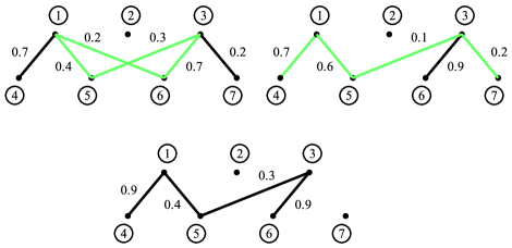
Figure 3.1. The process of changing a weighted bipartite graph to a bipartite graph with weights in $\left\{0,1\right\}$.

The figure on the upper left hand side shows the live edges of a bipartite graph on $7$ vertices. We pick a loop that is shown in green, and change the weights on it. We add $0.2$ to the weights of edges $\left\langle 1,5\right\rangle$ and $\left\langle 3,6\right\rangle$, and subtract $0.2$ from $w\left(\left\langle 5,3\right\rangle\right)$ and $w\left(\left\langle 6,1\right\rangle\right)$. Now, the edge $\left\langle 1,6\right\rangle$ dies and we get the figure on the upper right hand side. Since we have no other loops, we choose the biggest path that is shown in green. If we add and subtract $0.1$ to and from the weights of edges of this path alternatively, we get the third graph, where the edge $\left\langle 3,7\right\rangle$ becomes dead.

Lemma 3.19.

Let us define

$$D\left(i,A\right):=\sum_{j\in A\backslash\{i\}}\widetilde{p}_{ij},$$

where $i\in[n]$ and $A$ is a subset of $[n]=\left\{1,\cdots,n\right\}.$ Then, for every $A\subseteq[n]$, there is a bipartite graph $T$ with vertex sets $A$ and $B=[n]\backslash A$, and edges inside $Ed(A,B)$ such that

• (3.26) $$b_{i}\in\left\{\left\lfloor D\left(i,B\right)\right\rfloor,\,\left\lfloor D\left(i,B\right)\right\rfloor+1\right\},\text{ where }i\in A,$$

• and,

  (3.27) $$b_{i}\in\left\{\left\lfloor D\left(i,B\right)\right\rfloor,\,\left\lfloor D\left(i,B\right)\right\rfloor+1\right\},\text{ where }i\in B,$$

where $b_{i}$ is the degree of vertex $i$ in the graph $T$ and $\left\lfloor x\right\rfloor$ is the biggest integer less than $x$, for $x\in\mathbb{R}.$

Proof.

We already have a weighted bipartite graph $T$ with edge weights $0\leq\widetilde{p}_{ij}\leq 1$ that almost satisfies the conditions (3.26) and (3.27). Our goal is to change the weights continuously to get weights of size $0$ or $1$ without changing the degrees of our graph as much as possible. Let us denote the weight of an edge $e$ by $w(e)$. In addition, we say an edge $e$ is dead if $w(e)\in\left\{0,1\right\}$, and is live if $0<w(e)<1.$

Let us start a two stage process, where an example of that is shown at Fig. 3.1. We pick a closed loop of live edges, namely $e_{1},\cdots,e_{2k}$. Note that such a loop has an even number of edges since the graph $T$ is bipartite. Now, we add and subtract a constant number $c$ alternatively to the weights of $e_{i}$, for $1\leq i\leq k$, to get new weights $w(e_{1})+c,w(e_{2})-c,\cdots,$ and $w(e_{k})+(-1)^{k-1}c.$ Let $c$ grow gradually from $0$ until the first edge dies. Since the loop has an even length, the degrees of the graph have not changed. We keep on doing this until all loops disappear.

Next, we pick a path from the longest live paths in $T$. Suppose that the path runs through vertices $v_{1},\cdots,v_{k}$. We observe that if $v_{1}$ is attached to two live edges, we can either make our path longer or we get a loop amongst vertices $v_{i}$s. Since none of them are possible, $v_{1}$ is only attached to one live edge, and the same is true for $v_{k}$, the last vertex of the path. Again, we change the weights alternatively by $+c$ and $-c$, to get the new weights as $w(<v_{1},v_{2}>)+c,\,w(<v_{2},v_{3}>)-c,\cdots,$ and $w(<v_{k-1},v_{k}>)+(-1)^{k-1}c.$ Then, we let $c$ grow gradually until an edge dies. We repeat this process until no live edges are left.

Since the dead edges have a weight of 0 or 1, we have reached a bipartite graph. It remains to be shown that our new graph satisfies conditions (3.26) and (3.27). As we saw before, the degrees of vertices of $T$ do not change during the first stage of the process. Similarly, the degrees do not change in the second part, except for the end vertices of the paths. In addition, as we discussed earlier, if a vertex $v$ becomes an end point for a path in our procedure, that vertex is only attached to one live edge. Therefore, its degree $d(v)$ has changed by at most the amount of changes on the weight of that edge. Hence, $d(v)$ has became $\left\lfloor d(v)\right\rfloor$ or $\left\lfloor d(v)\right\rfloor+1$, which completes the proof.∎

Lemma 3.20.

If $\delta\leq\widetilde{p}_{ij}\leq 1-\delta$, for some $\delta>0,$ and $1\leq i,j,\leq n$, then,

$$P\left(\mathcal{\widetilde{G}}_{A}=\emptyset_{A}\right)\geq e^{-5\cdot\left|\log\left(\delta\right)\right|\cdot n\log^{\alpha}(n)},$$

where $A=I_{\alpha}$ and $B=[n]\backslash I_{\alpha}$, for some positive $\alpha$ (in particular $\alpha=\frac{10}{a_{1}}$), and $I_{\alpha}$ is as in Eq. (3.25). In addition, for the bipartite graph $T\subseteq Ed(A,B)$ in the previous lemma,

$$P\left(\mathcal{\widetilde{G}}_{A,B}=T\right)\geq e^{-5\cdot\left|\log\left(\delta\right)\right|\cdot n\log^{\alpha}(n)}.$$

Proof.

We have $d_{i}\leq\log^{\alpha}(n)$, for $i\in A$, and $\left|A\right|\leq n$. Therefore,

(3.28) $$S_{1}:=\sum_{i\in A}D(i,A)=\sum_{i\in A}\sum_{j\in A,j\neq i}\widetilde{p}_{ij}\leq\sum_{i\in A}d_{i}\leq n\log^{\alpha}(n).$$

Let $F_{1}$ be the set of edges $<i,j>$ in $Ed(A)$ such that $\widetilde{p}_{ij}>\frac{1}{2}.$ We see that $\left|F_{1}\right|\leq 2n\log^{\alpha}(n)$, otherwise, $S_{1}$ would exceed the right hand side of Eq. (3.28). Hence,

$$P(\mathcal{\widetilde{G}}_{A}=\emptyset_{A}) = \prod_{<i,j>\in Ed(A)}\left(1-\widetilde{p}_{ij}\right),$$

$$= \prod_{<i,j>\in F_{1}}\left(1-\widetilde{p}_{ij}\right)\cdot\prod_{<i,j>\in Ed(A)\backslash F_{1}}\left(1-\widetilde{p}_{ij}\right)$$

$$\geq \delta^{\left|F_{1}\right|}\prod_{<i,j>\in Ed(A)\backslash F_{1}}e^{-2\widetilde{p}_{ij}}$$

$$\geq \delta^{\left|F_{1}\right|}e^{-2S_{1}}$$

$$\geq e^{-\left(2\cdot\left|\log\left(\delta\right)\right|+2\right)\cdot n\log^{\alpha}(n)},$$

where we have used the inequality $1-x\geq e^{-2x}$, for $x\leq\frac{1}{2}$, and Eq. (3.28). This concludes the first part, since $\delta\leq\frac{1}{2}$ and $3\log(2)\geq 3\left|\log(\delta)\right|>2$.

For the second part, we define $F_{2}\subseteq Ed(A,B)$ similar to the set $F_{1}$, and

(3.29) $$S_{2}:=\sum_{i\in A}D\left(i,B\right)=\sum_{i\in A}\sum_{j\in B}\widetilde{p}_{ij}\leq\sum_{i\in A}d_{i}\leq n\log^{\alpha}\left(n\right).$$

Let $E$ be the set of edges of the graph $T$. Then,

$$P(\mathcal{\widetilde{G}}_{A,B}=T) = \prod_{<i,j>\in E}\widetilde{p}_{ij}\cdot\prod_{<i,j>\in Ed(A,B)\backslash E}\left(1-\widetilde{p}_{ij}\right),$$

$$\geq \delta^{\left|E\right|}.\prod_{<i,j>\in F_{2}}\left(1-\widetilde{p}_{ij}\right)\prod_{<i,j>\in Ed(A,B)\backslash\left(E\cup F_{2}\right)}\left(1-\widetilde{p}_{ij}\right)$$

$$\geq \delta^{\left|E\right|+\left|F_{2}\right|}\cdot\prod_{<i,j>\in Ed(A,B)\backslash F_{2}}e^{-\widetilde{p}_{ij}}$$

$$\geq \delta^{\left|E\right|+\left|F_{2}\right|}e^{-2S_{2}}.$$

Let us observe from the previous lemma that $\left|E\right|$, the number of edges of $T$, is less than or equal to $\frac{1}{2}S_{2}+n$. Using a bound on $F_{2}$ similar to that of $F_{1}$, and by (3.29) we get our result. ∎

In order to get the third part of Theorem (3.18), we use the union bound on the random graph $\mathcal{\widetilde{G}}_{B}$, where $B=[n]\backslash I_{\frac{10}{a_{1}}}$. Hence, the following proposition is handy.

Proposition 3.21.

For every $\alpha,\beta\in\mathbb{R}^{+},$ and large enough $n$ (depending on $\alpha$ and $\beta$), we have,

$$D\left(j,I_{\alpha}\right)<\frac{1}{4},$$

where $j\in I_{\beta},$ and $I_{\alpha}$ is as in Eq. (3.25).

Proof.

We prove this through a series of lemmas. Let us recall from the proof of Proposition 2.1 that, for the degree sequence $d_{1}\leq d_{2}\leq\cdots\leq d_{n}$, there exist positive real numbers $0<r_{1}\leq\cdots\leq r_{n}$ such that

$$\widetilde{p}_{ij}=\frac{r_{i}r_{j}}{1+r_{i}r_{j}},$$

and,

$$d_{i}=\sum_{j\in\left[n\right]\backslash\left\{i\right\}}\widetilde{p}_{ij},$$

where $\left[n\right]=\left\{1,\cdots,n\right\}.$ Also recall that $M=\sum_{i\leq n}d_{i}>n^{1+\epsilon}$, for large enough $n$. Moreover, let us assume that $I_{\alpha}=\left\{1,\cdots,k(\alpha)\right\}$, where $k(\alpha)$ is the number of elements of $I_{\alpha}$, and

(3.30) $$L_{\alpha}:=\left\{i:i\leq\ell(\alpha)\right\}\quad\text{with }\quad\ell(\alpha)=n-2d_{k(\alpha)}.$$

We note that $k(\alpha)\in I_{\alpha}$, and hence, $d_{k(\alpha)}\leq\log^{\alpha}\left(n\right).$ In addition, for large enough $n$,

$$\sum_{i=1}^{k(\alpha)}d_{i}+\sum_{i=\ell}^{n}d_{i} \leq k(\alpha)\cdot d_{k(\alpha)}+\left(2d_{k(\alpha)}+1\right)\cdot n$$

$$\leq n\cdot\log^{\alpha}\left(n\right)+\left(2\log^{\alpha}\left(n\right)+1\right)\cdot n$$

$$\leq n^{1+\epsilon}<M.$$

Therefore, $k(\alpha)<\ell(\alpha)$.

Now that the dependency of $I_{\alpha}$, $L_{\alpha}$, $k(\alpha)$, and $\ell(\alpha)$ on $\alpha$ is understood, we drop the $\alpha$ for the convenience of our notation, and use $I$, $L$, $k$ and $\ell$ throughout the rest of our proof.

Lemma 3.22.

For $j\in I$,

$$D(j,I)\leq 2d_{j}\frac{\sum_{i\in I}r_{i}}{\sum_{i\in L}r_{i}}.$$

Proof.

We see that $\widetilde{p}_{ij}=\frac{r_{i}r_{j}}{1+r_{i}r_{j}}$ is increasing both in $i$ and $j$ since $r_{i}$s are increasing in $i$, for $1\leq i,j\leq n$. Thus, it follows by Eq. (3.30) that

$$d_{k}\geq\sum_{j\geq\ell+1}\widetilde{p}_{kj}\geq 2d_{k}\widetilde{p}_{kl}.$$

This implies $\widetilde{p}_{kl}\leq\frac{1}{2}$ and therefore, for $i\leq k$ and $j\leq\ell$, we get $\widetilde{p}_{ij}\leq\frac{1}{2}$ and $r_{i}r_{j}\leq 1.$ We can now estimate for $j\leq\ell,$

$$D(j,I)=\sum_{i\leq k}\widetilde{p}_{ij}=\sum_{i\leq k}\frac{r_{i}r_{j}}{1+r_{i}r_{j}}\leq r_{j}\sum_{i\leq k}r_{i}.$$

Furthermore,

$$r_{j}=\frac{d_{j}r_{j}}{d_{j}}=\frac{d_{j}r_{j}}{\sum_{1\leq i\leq n}\frac{r_{i}r_{j}}{1+r_{i}r_{j}}}\leq\frac{d_{j}r_{j}}{\sum_{1\leq i\leq\ell}\frac{r_{i}r_{j}}{1+r_{i}r_{j}}}\leq\frac{2d_{j}r_{j}}{\sum_{1\leq i\leq\ell}r_{i}r_{j}}\leq\frac{2d_{j}}{\sum_{1\leq i\leq\ell}r_{i}}.$$

That does it.∎

Lemma 3.23.

We have,

$$\sum_{i\leq k}r_{i}\leq\sqrt{(4n+2)d_{k}}.$$

Proof.

Note that as in the previous lemma $r_{i}r_{j}\leq 1$, for $i\leq k$ and $j\leq\ell.$ Then, we observe that $k<\ell,$ and

$$\left[\sum_{i\leq k}r_{i}\right]^{2} = 2\sum_{i<j\leq k}r_{i}r_{j}+\sum_{i\leq k}r_{i}^{2}$$

$$\leq 4\sum_{i<j\leq k}\frac{r_{i}r_{j}}{1+r_{i}r_{j}}+\sum_{i\leq k}r_{i}r_{k}$$

$$\leq 4\sum_{i<j\leq k}\frac{r_{i}r_{j}}{1+r_{i}r_{j}}+2\sum_{i\leq k}\frac{r_{i}r_{k}}{1+r_{i}r_{k}}$$

$$\leq 4\sum_{i\leq k}d_{i}+2d_{k}$$

$$\leq \left(4n+2\right)d_{k}.$$

∎

Lemma 3.24.

For large enough $n$, we get

$$\sum_{i\leq\ell}r_{i}\geq\sqrt{\frac{M}{2}}.$$

Proof.

The proof goes through the following lines

$$\left[\sum_{i\leq\ell}r_{i}\right]^{2}\geq\sum_{1\leq i,j\leq\ell}\frac{r_{i}r_{j}}{1+r_{i}r_{j}}\geq\sum_{1\leq i,j\leq\ell}\widetilde{p}_{ij}\geq M-2\sum_{i>\ell}d_{i}\geq M-4nd_{k}.$$

Since $d_{k}\leq\log^{\alpha}\left(n\right)$, and $M>n^{1+\epsilon}$, we get our result for large enough $n$. ∎

Let us go back to the proof of our proposition. Since $k\in I_{\alpha}$ and $j\in I_{\beta}$, we have $d_{j}\leq\log^{\beta}\left(n\right)$ and $d_{k}\leq\log^{\alpha}\left(n\right)$. In addition, $M>n^{1+\epsilon}$, for large values of $n$. Combining the above three lemmas, we obtain

$$D(j,I)\leq 2d_{j}\sqrt{\frac{2\left(4n+2\right)d_{k}}{M}}\leq 8\frac{\log^{\beta+\frac{\alpha}{2}}\left(n\right)}{n^{\frac{\epsilon}{2}}}<\frac{1}{4},$$

for large enough $n$. ∎

We continue with the last part of Theorem 3.18. Recall that $\widetilde{\mathcal{G}}_{B}$ is the random graph with bernoulli random edges with parameter $\widetilde{p}_{ij}$, for $<i,j>\in Ed\left(B\right),$ where $B=\left[n\right]\backslash I_{\frac{10}{a_{1}}}$ and $0<a_{1}=a-\frac{1}{2}<\frac{1}{2}$.

Lemma 3.25.

Let $\mathbf{1}_{\left\langle i,j\right\rangle\in\mathcal{E}(G)}\left(G\right)$, for $i,j\in B$, be the indicator of the edge $\left\langle i,j\right\rangle$ in graph $G$. Then, we define the events,

(3.31) $$E_{j}:=\left\{G\text{ such that}\left|\sum_{i\in B}\mathbf{1}_{\left\langle i,j\right\rangle\in\mathcal{E}(G)}\left(G\right)-D(j,B)\right|\leq D(j,B)^{a}\right\},$$

and

(3.32) $$F_{j}:=\left\{G\text{ such that}\sum_{i\in B}\mathbf{1}_{\left\langle i,j\right\rangle\in\mathcal{E}(G)}\left(G\right)\leq\left(2\log^{2}(n)+1\right)D(j,B)\right\},$$

for $j\in B$. In addition, for $0<a_{1}=a-\frac{1}{2}<\frac{1}{2}$, we define

(3.33) $$J:=\left\{j\in\left[n\right]\big{|}\,D(j,B)\geq\log^{\frac{1}{a_{1}}}\left(n\right)\right\}.$$

Then, for large enough $n$,

$$P\left(\mathcal{\widetilde{G}}_{B}\in\cap_{j\in J}E_{j}\cap_{j\notin J}F_{j}\right)\geq 1-\frac{1}{n}>\frac{1}{2}.$$

Proof.

Let $X_{1},\cdots X_{n}$ be a vector of independent Bernoulli random variables with total mean $\mu:=\sum_{1\leq i\leq n}E\left[X_{i}\right]$. The Chernoff’s bound [15] states that, for $\delta>0$,

$$P\left(\sum_{1\leq i\leq n}X_{i}\geq(1+\delta)\mu\right)\leq\exp\left(\frac{-\mu\cdot\delta^{2}}{2+\delta}\right),$$

and

$$P\left(\sum_{1\leq i\leq n}X_{i}\leq(1-\delta)\mu\right)\leq\exp\left(\frac{-\mu\cdot\delta^{2}}{2+\delta}\right).$$

We apply Chernoff’s bound with parameters

$$\mu_{j}:=\sum_{i\in B\backslash\left\{j\right\}}E\left[\mathbf{1}_{\left\langle i,j\right\rangle}\right]=\sum_{i\in B\backslash\left\{j\right\}}\widetilde{p}_{ij}=D\left(j,B\right),$$

and $\delta=D\left(j,B\right)^{-\frac{1}{2}+a_{1}}\leq 1,$ where $1\leq j\leq n$. Hence,

(3.34) $$P\left(E_{j}^{c}\right)\leq 2\exp\left(-\frac{1}{3}D\left(j,B\right)^{2a_{1}}\right).$$

Now, for those $j$ in $J$ and by (3.33), we observe that Eq. (3.34) turns into

(3.35) $$P\left(E_{j}^{c}\right)\leq 2e^{-\frac{1}{3}\log^{2}\left(n\right)}.$$

Similarly, for $1\leq j\leq n$,

(3.36) $$P\left(F_{j}^{c}\right)\leq\exp\left(-\log^{2}(n)D\left(j,B\right)\right),$$

where $\delta=2\log^{2}(n)D\left(j,B\right).$ In order to complete the bound in Eq (3.36), we show $D(j,B)\geq\frac{1}{4},$ for $j\in B$. If $A=I_{\frac{10}{a_{1}}}=\left[n\right]\backslash B$ is empty then $D(j,B)=d_{j}\geq 1$. Otherwise, if $A\neq\emptyset$, then $1\in A$. We observe that $\frac{r_{i}r_{j}}{1+r_{i}r_{j}}$ is increasing both in $i$ and $j$, so

$$D(j,B) = \sum_{i\in B\backslash\left\{j\right\}}\widetilde{p}_{ij}=\sum_{i\in B\backslash\left\{j\right\}}\frac{r_{i}r_{j}}{1+r_{i}r_{j}}$$

$$\geq \sum_{i\in B}\left(\frac{r_{i}r_{1}}{1+r_{i}r_{1}}\right)-\frac{r_{1}r_{j}}{1+r_{1}r_{j}}$$

$$= D(1,B)-\widetilde{p}_{1j}$$

$$= d_{1}-D(1,A)-\widetilde{p}_{1j}.$$

In addition, we know that $d_{1}\geq 1$, and by Proposition 3.21, we get $D(1,A)\leq\frac{1}{4}$, for large enough $n$. Thus, if $\widetilde{p}_{1j}$ is smaller than $\frac{1}{4}$, then Eq. (3.2) gives $D(j,B)\geq\frac{1}{2}.$ On the other hand, we get $\frac{1}{4}\leq\widetilde{p}_{1j}\leq D(j,B)$.

Therefore,

$$P\left(F_{j}^{c}\right)\leq e^{-\frac{1}{4}\log^{2}\left(n\right)}.$$

Combining the previous inequality with Eq. (3.35), we have

$$P\left(\mathcal{\widetilde{G}}_{B}\in\cap_{j\in J}E_{j}\cap_{j\notin J}F_{j}\right)\geq 1-\sum_{i\in J}e^{-\frac{1}{3}\log^{2}\left(n\right)}-\sum_{i\notin J}e^{-\frac{1}{4}\log^{2}\left(n\right)}\geq 1-\frac{1}{n},$$

for large enough $n$. That concludes the proof.∎

Lemma 3.26.

Let $E_{j}$, $F_{j}$, and $J$ be as they are in Lemma 3.25. In addition, $T$ is the resulting bipartite graph in Lemma 3.19. Then, for every graph $G\in\cap_{j\in J}E_{j}\cap_{j\notin J}F_{j}$, we have

$$\emptyset_{A}\cup T\cup G\in\mathbb{G}_{a}^{D},$$

where $A=I_{\frac{10}{a_{1}}}$, and the graph $\emptyset_{A}$ is a graph on vertices of $A$ with no edges.

Proof.

Let us denote $d_{i}(G)$ by the degree of the $i^{th}$ vertex of the graph $G$. As usual, $B$ is $\left[n\right]\backslash A$. We need to show that

$$s_{i}:=\left|d_{i}-\left(d_{i}(\emptyset_{A})+d_{i}(T)+d_{i}(G)\right)\right|\leq 2d_{i}^{a},$$

for every $i\in\left[n\right].$ For $i\in A$, it follows by Lemma 3.19 and Proposition 3.21 that, for large enough $n$,

$$s_{i}=\left|d_{i}-d_{i}(T)\right|\leq 1+\left|d_{i}-D(i,B)\right|=D(i,A)+1<2.$$

Again, we let $J$ be the same as in (3.33). In addition, for $i\in J\cap B,$ we use the definition of $E_{j}$ (Eq. (3.31)), to get

$$s_{i} = \left|d_{i}-d_{i}(T)-d_{i}(G)\right|$$

$$\leq 1+\left|d_{i}-D(i,A)-d_{i}(G)\right|$$

$$= 1+\left|D(i,B)-d_{i}(G)\right|$$

$$\leq 1+D(i,B)^{a}$$

$$\leq 2d_{i}^{a}.$$

Last, for $i\in B\backslash J$, and using the property of the set $F_{i}$ (Eq. (3.32)), we obtain,

$$s_{i} = \left|d_{i}-d_{i}(T)-d_{i}(G)\right|$$

$$\leq 1+\left|D(i,B)-d_{i}(G)\right|$$

$$\leq 1+D(i,B)+\left(2\log^{2}\left(n\right)+1\right)D(i,B)$$

$$\leq 1+2\left(\log^{2}\left(n\right)+1\right)D(i,B).$$

Note that $i\notin J$, so $D(i,B)\leq\log^{\frac{1}{a_{1}}}\left(n\right)$, where $a_{1}=a-\frac{1}{2}$. In addition, $i\in B=\left[n\right]\backslash I_{\frac{10}{a_{1}}}$, where $I_{\frac{10}{a_{1}}}$ is defined by Eq. (3.25). Therefore, $d_{i}\geq\log^{\frac{10}{a_{1}}}\left(n\right)$, and

$$s_{i}\leq 8\log^{2+\frac{1}{a_{1}}}\left(n\right)\leq 2d_{i}^{a},$$

where we used $a<1$. This completes the proof. ∎

Proof of Theorem 3.18.

As we saw before, the partition is $A=I_{\frac{10}{a_{1}}}$, and $B=\left[n\right]\backslash A$, and $I_{\frac{10}{a}}$ is as in Eq. (3.25). Lemma 3.19 shows us that there exists a bipartite tree with edges in $Ed\left(A,B\right)$. From Lemma 3.20, we get parts a and b of the theorem.

Finally, putting Lemmas 3.25 and 3.26 together, we get the required lower bound for part c of the theorem.∎

3.3. Graphs with a given degree sequence.

Throughout this section, we let $C$ be a general constant. In addition, most of the proofs are analogous to the proof of Theorem 2.11 with some changes. So we provide an outline for each solution as well as the essential steps.

Recall that

$$\mathbf{p_{g}}\left(s,T\right)=E\left[\mathbf{1}_{s}\left(T,\mathcal{G}_{\mathbf{g}}\right)\right],$$

where $\mathcal{G}_{\mathbf{g}}$ is the random graph chosen uniformly in $\mathbb{G}^{D}$.

Corollary 3.27.

If we use the notation in Conjecture 2.19, then

$$\frac{1}{M}\cdot\sum_{\left(s,T\right)\in\mathbb{S}^{k}\times\mathbb{T}^{k}}\frac{1}{\psi(s,T,D)}\mathbf{p_{g}}\left(s,T\right)=k^{k-2}+O\left(\sqrt{\frac{n}{M}}\right).$$

Proof.

This is Theorem 2.16, when $a=0$. ∎

Proof of Remark 2.20.

Again, Lemma 3.7 implies that for a graph $G$ in $\mathbb{G}^{D}$,

$$P\left(\widetilde{\mathcal{G}}\left(D\right)=G\right)=\frac{\prod_{i=1}^{n}r_{i}^{d_{i}}}{\prod_{i,\,j}\left(1+r_{i}r_{j}\right)}=e^{-H_{1}\left(\widetilde{\mathbf{p}}\right)}$$

that is independent of the choice of the graph $G$. Therefore, conditioning on the event $\left\{\widetilde{\mathcal{G}}\left(D\right)\in\mathbb{G}^{D}\right\}$, the random graph $\widetilde{\mathcal{G}}\left(D\right)$ is exactly the random graph $\mathcal{G}_{\mathbf{g}}\left(D\right)$. In addition, suppose that Conjecture 2.18 holds that $e^{-\eta n\cdot\log(n)}\leq P\left(\widetilde{\mathcal{G}}\left(D\right)\in\mathbb{G}^{D}\right)$, for some $\eta>0$. Therefore,

$$P\left(\mathcal{G}_{\mathbf{g}}\left(D\right)\in A\right)=P\left(A|\widetilde{\mathcal{G}}\left(D\right)\in\mathbb{G}^{D}\right)\leq e^{\eta n\cdot\log(n)}P\left(\widetilde{\mathcal{G}}\left(D\right)\in A\right),$$

where $A$ is a subset of $\mathbb{G}^{D}$. The rest of the proof is almost identical to that of Theorem 2.11.

Lastly, the factor $O\left(n\log(n)\right)$ in the above equation ultimately provides us with a better bound, whereas in the proof of Theorem 2.11, we had $\mathcal{C}(D)$, which was of order $O(n^{a-\nu-\frac{1}{2}}\cdot M\cdot\log(n))$. ∎

3.4. Dense graphs (Definition 2.21).

Proof of theorem 2.23.

Suppose that the sequence $D$ satisfies the dense Erdös-Rényi condition for some positive numbers $c_{1}$, $c_{2}$ and $c_{3}$. Let $r_{i}$ be the variables defined in Eq. (3.3). Then, Lemma 4.1 in [6] implies

$$\log\left(\left|r_{i}\right|\right)<c_{4},$$

for $1\leq i\leq n$, and $c_{4}$ is a number that depends on $c_{1}$, $c_{2}$ and $c_{3}$.

Therefore, for $\mathcal{C}_{2}\left(D\right)$ as in Eq. (3.7),

$$\mathcal{C}\left(D\right)=\sum_{i=1}^{n}d_{i}^{a}\left|\log(r_{i})\right|<c_{4}\sum_{i=1}^{n}d_{i}^{a}.$$

Using Cauchy-Schwarz, and that $d_{i}<n$, for $1\leq i\leq n$, we get $\mathcal{C}_{2}(D)<C\sqrt{\frac{n}{M}}n^{a-\frac{1}{2}}$ $<Cn^{-\frac{1}{2}+a}$ . Similarly, we get a better bound for $\mathcal{C}_{1}\left(D\right)$ (3.5). From here, the solution is as follows in Remark 3.14 and, hence,

$$\sum_{\left(s,T\right)\in\mathbb{S}^{k}\times\mathbb{T}^{k}}\frac{1}{\psi(s,T,D)}\left|\mathbf{p_{\mathbf{a}}}\left(s,T\right)-\mathbf{\widetilde{p}}\left(s,T\right)\right|\leq C_{k}\cdot n^{\frac{-1}{4}+\left(a-\frac{1}{2}\right)},$$

where $C_{k}>0$ is a constant depending on $k$. That completes the second part of the theorem.

As for the first part of the theorem, we can either use lemma 6.2 in [6] or an exact bound from Theorem 1.4 in [1] to show that Conjecture 2.18 holds. We consider the latter here. Again, for $1\leq i,j\leq n$, the numbers $r_{i}$s are bounded, and so are the numbers $\widetilde{p}_{ij}=\frac{r_{i}r_{j}}{1+r_{i}r_{j}}$, the entries of the maximum entropy. In addition, for some $\delta(c_{4})$ and as it was discussed in Remark 2.22, we have $\delta\leq\widetilde{p}_{ij}\leq 1-\delta$, which means that the maximum entropy vector $\widetilde{\mathbf{p}}$ is $\delta-tame$. Now, Theorem 1.4 in [1] states,

$$P\left(\widetilde{G}\in\mathbb{G}^{D}\right)=e^{-H_{1}(\widetilde{p})}\left|\mathbb{G}^{D}\right|\approx\frac{2}{\left(2\pi\right)^{n/2}\sqrt{Q}}e^{-\frac{\mu}{2}+\nu}\geq Ce^{-\gamma n\log(n)}.$$

Look at [1] for a precise definition of the variables. But let us just note that $\mu$ and $\nu$ are constants depending on $D$, and bounded by $\delta$. Also, the variable $Q$ is the determinant of a $n\times n$ matrix with entries bounded from below and above by constants depending on $\delta$. Using Hadamard’s inequality [25] to bound the determinant, we get the lower bound that we needed, which is

$$Ce^{-\eta n\log(n)}\leq P(\widetilde{\mathcal{G}}\left(D\right)\in\mathbb{G}^{D}),$$

for some constants $C$ and $\eta>0$. The rest is similar to the proof of Remark2.20 and 2.11. ∎

3.5. Very Sparse graphs ( Definition 2.24).

Effectively, the proof of Theorem 2.25 is a repetition of the arguments in the proof of Theorem 2.11, although with slight changes. We start by giving the counterparts of Lemma 3.7 and Proposition 3.6. The idea is to use $\frac{d_{i}}{\sqrt{M}}$ as $r_{i}$, for $1\leq i\leq n$, so $\widetilde{p}_{ij}=\frac{r_{i}r_{j}}{1+r_{i}r_{j}}$ becomes $q_{ij}=\frac{d_{i}d_{j}}{M+d_{i}d_{j}}.$

Recall that $\mathcal{G}_{q}$ is a random graph with independent Bernoulli random edges with parameters $q{}_{ij}$, and

$$\mathbf{p_{q}}\left(s,T\right)=E\left[\mathbf{1}_{s}\left(T,\mathcal{G}_{\mathbf{q}}\left(D\right)\right)\right].$$

We state some lemmas.

Lemma 3.28.

With the same notation as above,

1. let $d_{\mathbf{q}}\left(i\right):=\sum_{j=1,j\neq i}^{n}q_{ij}$, then $d_{q,i}=d_{i}\left(1-O(\frac{d_{n}^{2}}{M})\right)$, or more precisely,

   $$d_{i}\left(1-\frac{2d_{n}^{2}}{M}\right)\leq d_{i}\left(1-\frac{2d_{i}d_{n}}{M}\right)\leq d_{q,i}\leq d_{i}.$$

2. For a given graph $G$ with the degree sequence $D(G):=\left\{\hat{d}_{1}(G),\cdots,\hat{d}_{n}(G)\right\}$ that may differ from $D=\left\{d_{1},\cdots d_{n}\right\},$ we get

   $$P\left(\mathcal{G}_{\mathbf{q}}\left(D\right)=G\right)=\frac{\prod_{i=1}^{n}\left(\frac{d_{i}}{\sqrt{M}}\right)^{\hat{d}_{i}(G)}}{\prod_{1\leq i<j\leq n}\left(1+\frac{d_{i}d_{j}}{M}\right)}.$$

3. Define

   $$P_{q,\min}=\min_{G\in\mathbb{G}_{a}^{D}}P\left(\mathcal{G}_{\mathbf{q}}\left(D\right)=G\right)\textit{ and }P_{q,\max}=\max_{G\in\mathbb{G}_{a}^{D}}P\left(\mathcal{G}_{\mathbf{q}}\left(D\right)=G\right),$$

   then,

   $$\left|\log\left(\frac{P_{q,\max}}{P_{q,\min}}\right)\right|\leq 2\log(n)\sum_{i=1}^{n}\left(d_{i,q}\right)^{a}.$$

   Moreover, $\sum_{i=1}^{n}d_{i}^{a}\leq\left(\frac{M}{n}\right)^{\frac{1}{2}}n^{\left(a-\frac{1}{2}\right)}$.

Proof.

1. First, consider the following expression for $d_{i}-d_{\mathbf{q}}\left(i\right)$,

   $$d_{i}-\sum_{j\neq i,j\in\left[n\right]}q_{ij} = \frac{d_{i}}{M}\sum_{j=1}^{n}d_{j}-\sum_{j=1,j\neq i}^{n}\frac{d_{i}d_{j}}{M+d_{i}d_{j}}$$

   $$= \frac{d_{i}^{2}}{M}+\sum_{j=1,j\neq i}^{n}\frac{d_{i}^{2}d_{j}^{2}}{M\left(M+d_{i}d_{j}\right)}$$

   $$< \frac{d_{i}^{2}}{M}\left(1+\sum_{j\neq i}\frac{d_{n}d_{j}}{M}\right)$$

   $$< d_{i}^{2}\frac{2d_{n}}{M}<d_{i}\frac{2d_{n}^{2}}{M}.$$

   Second, note that the difference is positive as it is shown in the second step of the above equation.

2. This is part 2 of Lemma 3.7, when $r_{i}$s are replaced by $\frac{d_{i}}{\sqrt{M}}$s.

3. The proof follows from the second part of this lemma, Eq. (3.8) and (3.7), and the fact that $\log(\frac{d_{i}}{\sqrt{M}})$ is bounded by $\log(n)$.

∎

Lemma 3.29.

There exits $\eta>0$ such that, for large enough $n$,

$$-\eta\left(n\log(n)+\frac{d_{n}^{4}}{M}\right)\leq\log\left(P\left(\mathcal{G}_{\mathbf{q}}\left(D\right)\in\mathbb{G}^{D}\right)\right)\leq\log\left(P\left(\mathcal{G}_{\mathbf{q}}\left(D\right)\in\mathbb{G}_{a}^{D}\right)\right).$$

Proof.

It follows from the part two of the previous lemma that,

(3.38) $$P\left(\mathcal{G}_{\mathbf{q}}\left(D\right)\in\mathbb{G}^{D}\right)=\left|\mathbb{G}^{D}\right|\cdot e^{L},$$

where

$$L=\sum_{i=1}^{n}d_{i}\left(\ln\left(d_{i}\right)-\frac{1}{2}\ln\left(M\right)\right)-\sum_{1\leq i<j\leq n}\ln\left(1+\frac{d_{i}d_{j}}{M}\right),$$

and also, $L=P\left(\mathcal{G}_{\mathbf{q}}\left(D\right)=G\right)$ for any graph $G\in\mathbb{G}^{D}$.

Next, we use Theorem 4.6 in [26], which gives the number of graphs with a given degree sequence $D$. Hence,

(3.39) $$P\left(\mathcal{G}_{\mathbf{q}}\left(D\right)\in\mathbb{G}^{D}\right)=\frac{M!\exp\left(-\lambda-\lambda^{2}+O(\frac{d_{n}^{2}}{M})\right)}{\left(\frac{M}{2}\right)!2^{\left(\frac{M}{2}\right)}\prod_{i=1}^{n}d_{i}!}\cdot e^{L},$$

where $\lambda$ is $\frac{1}{M}\sum_{i=1}^{n}\left(\begin{array}[]{c}d_{i}\\ 2\end{array}\right)$. We put Eqs. (3.38) and(3.39) together, and use the stirling estimate that is

$$\log\left(n!\right)-n\log\left(n\right)+n-\frac{1}{2}\log\left(2\pi n\right)\leq\frac{c}{n},$$

where $c>0$.

Thus, for $M=\sum_{i=1}^{n}d_{i}$ and $d_{i}\geq 1$,

(3.40) $$\log \left(P\left(\mathcal{G}_{\mathbf{q}}\left(D\right)\in\mathbb{G}^{D}\right)\right)$$

$$\geq L-\lambda-\lambda^{2}+O\left(\frac{d_{n}^{2}}{M}\right)+M\log\left(M\right)-M+\frac{1}{2}\log\left(2\pi M\right)$$

$$-\left(\frac{M}{2}\log\left(\frac{M}{2}\right)-\frac{M}{2}+\frac{1}{2}\log\left(2\pi\frac{M}{2}\right)+\frac{c}{M}\right)-\frac{M}{2}\log\left(2\right)$$

$$-\sum_{i=1}^{n}\left(d_{i}\log\left(d_{i}\right)-d_{i}+\frac{1}{2}\log\left(2\pi d_{i}\right)+\frac{c}{d_{i}}\right)$$

$$\geq -\sum_{1\leq i<j\leq n}\ln\left(1+\frac{d_{i}d_{j}}{M}\right)-\lambda-\lambda^{2}+O\left(\frac{d_{n}^{2}}{M}\right)+\frac{M}{2}+\frac{1}{2}\log(2)$$

$$-\frac{n}{2}\log\left(2\pi\right)-\frac{1}{2}\sum_{i=1}^{n}\log\left(d_{i}\right)-c\left(n+1\right).$$

It is time for the Taylor series for $\log(1+\frac{d_{i}d_{j}}{M})$, which is possible because $\frac{d_{i}d_{j}}{M}<\frac{d_{n}^{2}}{M}<1$. So, for $\lambda=\frac{1}{2M}\sum_{i=1}^{n}\left(d_{i}^{2}-d_{i}\right)=\frac{1}{2M}\sum_{i=1}^{n}d_{i}^{2}-\frac{1}{2},$

(3.41) $$I:= \sum_{1\leq i<j\leq n}\ln\left(1+\frac{d_{i}d_{j}}{M}\right)+\lambda+\lambda^{2}$$

$$\leq \sum_{1\leq i<j\leq n}\left(\frac{d_{i}d_{j}}{M}-\frac{1}{2}\left(\frac{d_{i}d_{j}}{M}\right)^{2}+\frac{1}{3}\left(\frac{d_{i}d_{j}}{M}\right)^{3}\right)+\frac{1}{2M}\sum_{i=1}^{n}d_{i}^{2}-\frac{1}{2}$$

$$+\left(\frac{1}{2M}\sum_{i=1}^{n}d_{i}^{2}-\frac{1}{2}\right)^{2}$$

$$= \frac{1}{2M}\left(\sum_{i=1}^{n}d_{i}\right)^{2}-\frac{1}{2}+\sum_{1\leq i<j\leq n}\left(-\frac{1}{2M^{2}}d_{i}^{2}d_{j}^{2}+\frac{1}{3M^{3}}d_{i}^{3}d_{j}^{3}\right)$$

$$+\frac{1}{4M^{2}}\sum_{i=1}^{n}d_{i}^{4}+\frac{1}{2M^{2}}\sum_{1\leq i<j\leq n}d_{i}^{2}d_{j}^{2}-\frac{1}{2M}\sum_{i=1}^{n}d_{i}^{2}+\frac{1}{4}$$

$$= \frac{M}{2}-\frac{1}{4}+\frac{1}{3M^{3}}\sum_{1\leq i<j\leq n}d_{i}^{3}d_{j}^{3}+\frac{1}{4M^{2}}\sum_{i=1}^{n}d_{i}^{4}-\frac{1}{2M}\sum_{i=1}^{n}d_{i}^{2}$$

$$\leq \frac{M}{2}+\frac{d_{n}^{4}}{3M^{3}}\sum_{1\leq i<j\leq n}d_{i}d_{j}+\frac{d_{n}^{3}}{4M^{2}}\sum_{i=1}^{n}d_{i}$$

$$\leq \frac{M}{2}+\frac{d_{n}^{4}}{M}.$$

Combining (3.40) and (3.41), we get

$$\log\left(P\left(\mathcal{G}_{\mathbf{q}}\left(D\right)\in\mathbb{G}^{D}\right)\right)\geq-\frac{d_{n}^{4}}{M}-\frac{n}{2}\log\left(2\pi\right)-\frac{1}{2}n\log\left(n\right)-c\left(n+1\right),$$

where we used $d_{i}<n$. That concludes the lemma. ∎

Next, we see the sparse version of Theorem 2.16, which follows from the proof of Theorem 2.25.

Lemma 3.30.

The sum of variables in Theorem 2.25 is nearly constant, i.e.

$$\frac{1}{M}\cdot\sum_{\left(s,T\right)\in\mathbb{S}^{k}\times\mathbb{T}^{k}}\frac{1}{\psi(s,T,D)}\mathbf{p_{q}}\left(s,T\right)=k^{k-2}+O\left(\sqrt{\frac{n}{M}}\right)+O\left(\frac{d_{n}^{2}}{M}\right),$$

where the constant in the $O$ notation may depend on $k$.

Proof.

Let $D_{\mathbf{q}}$ be the vector $\left(d_{\mathbf{q}}\left(i\right)\right)$, where $1\leq i\leq n$, and $M_{\mathbf{q}}:=\sum_{i=1}^{n}d_{\mathbf{q}}\left(i\right)$. Replacing $\widetilde{p}_{ij}$ with $q_{ij}$ in Theorem 3.27, we get

$$\frac{1}{M_{\mathbf{q}}}\cdot\sum_{\left(s,T\right)\in\mathbb{S}^{k}\times\mathbb{T}^{k}}\frac{1}{\psi(s,T,D_{\mathbf{q}})}\mathbf{p_{q}}\left(s,T\right)=k^{k-2}+O\left(\sqrt{\frac{n}{M_{q}}}\right).$$

Recall that

$$\psi(s,T,D)=\prod_{u\in V(T)}d_{s(u)}^{b_{u}-1},$$

where $\mathcal{V}(T)$ is the vertex set of $T\in\mathbb{T}^{k}$, and $b_{u}$ is the degree of a vertex $u$ in $\mathcal{V}(T)$. Thus, the first part of Lemma 3.28 demonstrates that

$$1\leq\frac{\psi(s,T,D)}{\psi(s,T,D_{\mathbf{q}})}\leq\left(1-\frac{2d_{n}^{2}}{M}\right)^{-k}\leq 1+2k\cdot\frac{d_{n}^{2}}{M},$$

and that $\left(1-\frac{2d_{n}^{2}}{M}\right)\leq\frac{M_{q}}{M}\leq 1.$ The combination of the above equations concludes this lemma. ∎

Lemma 3.31.

We let $A$ be any subset of $\mathbb{S}_{n}^{k}\times\mathbb{T}^{k}$. Then, for $\epsilon<<1$,

$$P\left(\left|\frac{1}{M}\cdot\sum_{\left(s,T\right)\in A}\frac{1}{\psi(s,T,D)}\left(\mathbf{p_{q}}\left(s,T\right)-\mathbf{1}_{s}\left(T,\mathcal{G}_{\mathbf{q}}\left(D\right)\right)\right)\right|>\mu\epsilon\right)\leq e^{-\left(c\mu M\right)\epsilon^{2}},$$

where

$$\mu:=\frac{1}{M}\cdot\sum_{\left(s,T\right)\in A}\frac{1}{\psi(s,T,D)}\mathbf{p_{q}}\left(s,T\right).$$

Proof.

We use the the estimate $\frac{d_{\mathbf{q}}\left(i\right)}{d_{i}}=\Theta(1-\frac{2d_{n}^{2}}{M})$ from part 1 of Lemma 3.28 to interchange between $d_{i}$ and $d_{\mathbf{q}}\left(i\right)$. Other than that the proof is a repetition of Lemma 3.3, which we skip. ∎

Proof of Theorem 2.25.

We know that $d_{n}^{2}=o(M)$, hence $d_{n}^{2}<\frac{1}{2}M$ eventually. The first part follows from Remark 2.13 and 2.11.

Next, we show that

$$I: = \sum_{\left(s,T\right)\in\mathbb{T}^{k}\times\mathbb{S}^{k}}\frac{1}{\psi(s,T,D)}\left|\mathbf{p_{\mathbf{q}}}\left(s,T\right)-\mathbf{p_{a}}\left(s,T\right)\right|$$

$$\leq C_{k}\cdot\left(\left(\frac{n}{M}\right)^{1/4}n^{a_{1}}+\frac{d_{n}^{2}}{M}\right),$$

where $a_{1}:=\left(a-\frac{1}{2}\right)$ and $C_{k}>0$ are constants. We combine Lemma 3.30 and Theorem 2.16 as usual. We get an equation related to Eq. (3.21) that is

$$I=2\left[\sum_{\left(s,T\right)\in A^{-}}\frac{1}{\psi(s,T,D)}\left(\mathbf{p_{\mathbf{q}}}\left(s,T\right)-\mathbf{p_{a}}\left(s,T\right)\right)\right]+O\left(\left(\frac{n}{M}\right)^{1/2}n^{a_{1}}+\frac{d_{n}^{2}}{M}\right),$$

where

$$A^{-}=\left\{\left(s,T\right)\in\mathbb{S}_{n}^{k}\times\mathbb{T}^{k}\Big{|}\mathbf{p_{\mathbf{q}}}\left(s,T\right)-\mathbf{p_{a}}\left(s,T\right)>0\right\}.$$

Now, we follow the streamline in the proof of Theorem 2.11. Much like (3.22) and without a loss of generality, we assume that the variable

$$\mu_{\mathbf{q}}^{-}:=\sum_{\left(s,T\right)\in A^{-}}\frac{1}{\psi(s,T,D)}\mathbf{p_{\mathbf{q}}}\left(s,T\right)$$

is greater or equal to $\left(\frac{n}{M}\right)^{1/2}n^{3a_{1}}$. In addition, we let $\epsilon$ satisfy

$$\epsilon^{2}=\frac{1}{\mu_{\mathbf{q}}^{-}}\left(\frac{n}{M}\right)^{1/2}n^{2a_{1}},$$

which resembles Eq. (3.22) with $n^{-\nu}=\sqrt{\frac{n}{M}}$.

We continue and combine part 3 and 4 of Lemma 3.28, and Lemma 3.31 to get,

$$L^{-}$$

$$:=P\left(\left|\sum_{\left(s,T\right)\in A^{-}}\frac{1}{\psi(s,T,D)}\left(\mathbf{p}_{\mathbf{q}}\left(s,T\right)-\mathbf{1}_{s}\left(T,\mathcal{G}_{\mathbf{a}}\left(a,D\right)\right)\right)\right|>\mu^{-}\epsilon\right)$$

$$\leq\frac{\exp\left(O(\left(\frac{M}{n}\right)^{\frac{1}{2}}n^{a_{1}})\right)}{P\left(\mathcal{G}_{\mathbf{q}}\in\mathbb{G}_{a}^{D}\right)}P\left(\left|\sum_{\left(s,T\right)\in A^{-}}\frac{1}{\psi(s,T,D)}\left(\mathbf{p}_{\mathbf{q}}\left(s,T\right)-\mathbf{1}_{s}\left(T,\mathcal{G}_{\mathbf{q}}\right)\right)\right|>\mu^{-}\epsilon\right)$$

$$\leq\exp\left(-\left(c\mu M\right)\epsilon^{2}+O\left(\left(\frac{M}{n}\right)^{\frac{1}{2}}n^{a_{1}}\right)+O\left(n\log(n)\right)\right),$$

where $\mathcal{G}_{\mathbf{q}}=\mathcal{G}_{\mathbf{q}}\left(D\right)$. The rest is the same process as in the proof of Theorem 2.11, and we end up with the bound in Eq. (3.5), i.e.

$$I\leq C_{k}\cdot\left(\left(\frac{n}{M}\right)^{1/4}n^{a_{1}}+\frac{d_{n}^{2}}{M}\right).$$

For the last parts of our theorem, we use part 1 of Lemma 3.28. Therefore,

$$P\left(\mathcal{G}_{\mathbf{q}}\left(D\right)\in A\right) = P\left(\mathcal{G}_{\mathbf{q}}\left(D\right)\in A\Big{|}\mathcal{G}_{\mathbf{q}}\left(D\right)\in\mathbb{G}^{D}\right)$$

$$\leq \frac{1}{P\left(\mathcal{G}_{\mathbf{q}}\left(D\right)\in\mathbb{G}^{D}\right)}P\left(\mathcal{G}_{\mathbf{q}}\left(D\right)\in A\right),$$

where $A$ is a subset of $\mathbb{G}^{D}$, and again, $\mathcal{G}_{\mathbf{g}}$ is the random graph chosen uniformly from $\mathbb{G}^{D}$. Using Eq. 3.5, the last part of Lemma 3.28, and an argument identical to the proof of Remark 2.20, we obtain

(3.44) $$\sum_{\left(s,T\right)\in\mathbb{S}_{n}^{k}\times\mathbb{T}^{k}}\frac{1}{\psi(s,T,D)}\left|\mathbf{p_{\mathbf{q}}}\left(s,T\right)-\mathbf{p_{g}}\left(s,T\right)\right|\leq C_{k}\cdot\left(\left(\frac{n\log(n)}{M}\right)^{1/2}+\frac{d_{n}^{2}}{M}\right),$$

where

$$\mathbf{p_{g}}\left(s,T\right)=E\left[\mathbf{1}_{s}\left(T,\mathcal{G}_{\mathbf{g}}\right)\right],$$

as in Conjecture 2.19.

Finally, parts 2 and 3 of the theorem follow from the first part of the theorem, Eq. (3.5) and (3.44), and the triangle inequality. ∎

Remark 3.32.

Although the bound for the differences $\left|\mathbf{p_{g}}\left(s,T\right)-\mathbf{\widetilde{p}}\left(s,T\right)\right|$ in the second part of the theorem is $o(1)$, compared to Conjecture 2.19, it is not optimal. The reason is that we do not get the lower bound in Conjecture 2.18. Instead, we use parameters $\mathbf{p_{q}}\left(s,T\right)$ and $\mathbf{p_{a}}\left(s,T\right)$ as a middle step to achieve our bound.

3.6. Bipartite graphs (proof of Theorem 2.30).

Although the setup is a little bit different here, the proof operates along similar lines as the proof of Remark 2.20. The main difference is that everything splits into two sets of variables. For example, there is a related version of Eq. (3.4) for the maximum entropy $\widetilde{\mathbf{p}}\in\mathbb{P}^{D_{1},D_{2}}$. We write, for $1\leq i\leq n_{1}$ and $1\leq j\leq n_{2}$,

$$\widetilde{p}_{ij}=\frac{r_{1,i}r_{2,j}}{1+r_{1,i}r_{2,j}},$$

where $x^{\ast}=(r_{1,1},...,r_{1,n_{1}})$ and $y^{\ast}=(r_{2,1},...,r_{2,n_{2}})$ are two positive vectors.

In regard to the ordered trees, we restrict our sums to the trees $\left(s,T\right)\in\mathbb{S}_{n}^{k}\times\mathbb{T}^{k}$ that $s\left(T\right)$ does not have any edge with both ends in vertices of either part $1$ or part $2$. We let $\mathcal{T}_{\mathbf{b}}^{k}$ be the set of such trees. We check that

(3.45) $$\frac{1}{M}\cdot\sum_{\left(s,T\right)\in\mathcal{T}_{\mathbf{b}}^{k}}\frac{1}{\psi(s,T,D)}\mathbf{p_{b}}\left(s,T\right)=k^{k-2}+O\left(\sqrt{\frac{n}{M}}\right)$$

is still valid. Although it sounds contradictory to Theorem 3.27 since $\mathcal{T}_{\mathbf{b}}^{k}$ is a subset of $\mathbb{S}_{n}^{k}\times\mathbb{T}^{k}$, we note that the definitions of $d_{1,i}$ and $d_{2,i}$ are different from $d_{i}$ in Theorem 3.27. Here,

$$d_{1,i}:=\sum_{j=1}^{n_{1}}\widetilde{p}_{ij},\text{ and }d_{2,i}:=\sum_{i=1}^{n_{2}}\widetilde{p}_{ij},$$

as opposed to

$$d_{i}:=\sum_{i=1}^{n}\widetilde{p}_{ij},$$

where $n=n_{1}+n_{2}$.

Next, Theorem 1-1 of [1] gives the following bounds

(3.46) $$(n_{1}n_{2})^{-\eta(n_{1}+n_{2})}\leq P\left(\mathcal{G}_{\mathbf{b}}\left(D_{1},D_{2}\right)\in\mathbb{G}^{D_{1},D_{2}}\right)=e^{-H_{2}\left(\widetilde{\mathbf{p}}\right)}\left|\mathbb{G}^{D_{1},D_{2}}\right|,$$

for some positive $\eta$ independent of $n$. The above term $(n_{1}n_{2})^{-\eta(n_{1}+n_{2})}$ is bounded by $e{}^{-\eta n\log(n^{2})}$. Equations (3.45) and (3.46) are enough to produce a proof using the same method in the proof of Remark 2.20, and we skip the details.

Remark 3.33.

The Theorem 1-1 of [1] only requires that the polytope $\mathbb{P}^{D_{1},D_{2}}$ has a non-empty interior. That gives a proof of Theorem 2.30 without any extra conditions on the degree sequence like part 2 and 3 of Assumption 2.7. We also believe that one can prove all the previous results without any extra condition on the degree sequence.

4. Acknowledgements

The author would like to thank S. R. Srinivasa Varadhan for reviewing the manuscript and his useful comments. Thanks to S. Chatterjee for suggesting the problem. Thanks to A. Barvinok, M. Harel, A. Krishnan, and A. Munez for fruitful discussions and references.

Appendix A A concentration inequality.

We also need the following concentration theorem for the proof of Theorem 2.11 that is inspired by a paper by Janson [21]. This is the generalized version of Theorem 1 from Janson’s paper, and we modified the proof for our purpose. Therefore, we begin this part with some notations and a theorem.

Consider a set $\left\{J_{i}\right\}_{i\in Q}$ of independent random indicator variables and a family $\left\{Q(\alpha)\right\}_{\alpha\in A}$of subsets of the index set $Q$, and define $\mathbf{1}_{\alpha}=\prod_{i\in Q(\alpha)}J_{i}$ and $S=\sum_{\alpha\in A}\frac{1}{\omega_{\alpha}}\mathbf{1}_{\alpha}$, where $\omega_{\alpha}$ are positive numbers. [In other words, $S$ counts the weighted number of the given sets $Q\{\alpha\}$ that are contained in the random set $\left\{i\in Q:\,J_{i}=1\right\}$, with independently appearing elements.] We assume, for the sake of simplicity, that the index set $A$ is finite, but it is easy to see that the results extend to infinite sums, provided $E[S]<\infty$.

Write $\alpha\sim\beta$ if $Q(\alpha)\cap Q(\beta)\neq\emptyset$ but $\alpha\neq\beta$, and define

$$p_{\alpha}=E\left[\mathbf{1}_{\alpha}\right],$$

$$\lambda=E\left[S\right]=\sum\frac{1}{\omega_{\alpha}}p_{\alpha},$$

$$\delta_{1}=\frac{1}{\lambda}\sum_{\alpha}\frac{p_{\alpha}}{\omega_{\alpha}^{2}},$$

$$\delta_{2}=\frac{1}{\lambda}\sum_{\alpha}\sum_{\beta\sim\alpha}\frac{1}{\omega_{\alpha}\omega_{\beta}}E\left[\mathbf{1}_{\alpha}\mathbf{1}_{\beta}\right].$$

Theorem A.1.

With notation above and $0\leq\epsilon\leq 1$ then

$$P(S\leq(1-\epsilon)\lambda)\leq\exp\left[-\frac{\lambda}{\delta_{1}+\delta_{2}}(\epsilon+(1-\epsilon)\log(1-\epsilon))\right].$$

We want to use the Chernoff bound, but first we need an upper bound for the moment-generating function. So the proof of Theorem A.1 follows our next lemma.

Lemma A.2.

Using the preceding notations in Theorem A.1 and for $t\geq 0$, we have

$$E\left[e^{-tS}\right]\leq\exp\left[-\frac{\lambda}{\delta_{1}+\delta_{2}}(1-e^{-(\delta_{1}+\delta_{2})t})\right].$$

Proof.

Let $\psi(t)=E\left[e^{-tS}\right]$, for $t\geq 0$. Then

$$-\frac{d\psi(t)}{dt}=E\left[Se^{-tS}\right]=\sum_{\alpha}E\left[\frac{1}{\omega_{\alpha}}\mathbf{1}_{\alpha}e^{-tS}\right].$$

We split $S$ into two parts; the part that is dependent on $\mathbf{1}_{\alpha}$: $S^{\prime}_{\alpha}=\frac{1}{\omega_{\alpha}}\mathbf{1}_{\alpha}+\sum_{\alpha\sim\beta}\frac{1}{\omega_{\beta}}\mathbf{1}_{\beta}$ , and $S^{\prime}_{\alpha}=S-S^{\prime}_{\alpha}$, which is independent of $\mathbf{1}_{\alpha}$. Thus,

$$E\left[\mathbf{1}_{\alpha}e^{-tS}\right]=p_{\alpha}E\left[e^{-tS^{\prime}_{\alpha}-tS^{\prime\prime}_{\alpha}}\big{|}\mathbf{1}_{\alpha}=1\right].$$

The event $\mathbf{1}_{\alpha}=1$ fixes $J_{i}:i\in Q(\alpha)$. Since $e^{-tS^{\prime}_{\alpha}}$ and $e^{-tS^{\prime\prime}_{\alpha}}$ are decreasing functions of the remaining $J_{i}:\,i\in Q$, using the FKG inequality we get

(A.1) $$E\left[\mathbf{1}_{\alpha}e^{-tS}\right] \geq p_{\alpha}E\left[e^{-tS^{\prime}_{\alpha}}\big{|}\mathbf{1}_{\alpha}=1\right]E\left[e^{-tS^{\prime\prime}_{\alpha}}\big{|}\mathbf{1}_{\alpha}=1\right]$$

$$= p_{\alpha}E\left[e^{-tS^{\prime}_{\alpha}}\big{|}\mathbf{1}_{\alpha}=1\right]E\left[e^{-tS^{\prime\prime}_{\alpha}}\right]$$

$$\geq p_{\alpha}E\left[e^{-tS^{\prime}_{\alpha}}\big{|}\mathbf{1}_{\alpha}=1\right]\psi(t).$$

Now summing over $\alpha$ and using Jensen’s inequality twice we have

(A.2) $$-\frac{d\log(\psi(t))}{dt} = \frac{1}{\psi(t)}\sum_{\alpha}\frac{1}{\omega_{\alpha}}E\left[\mathbf{1}_{\alpha}e^{-tS}\right]\geq\sum_{\alpha}\frac{p_{\alpha}}{\omega_{\alpha}}E\left[e^{-tS^{\prime}_{\alpha}}\big{|}\mathbf{1}_{\alpha}=1\right]$$

$$\geq \sum_{\alpha}\frac{p_{\alpha}}{\omega_{\alpha}}\exp\left[-tE\left[S^{\prime}_{\alpha}\big{|}\mathbf{1}_{\alpha}=1\right]\right]$$

$$= \lambda\sum_{\alpha}\frac{1}{\lambda}\frac{p_{\alpha}}{\omega_{\alpha}}\exp\left[-tE\left[S^{\prime}_{\alpha}\big{|}\mathbf{1}_{\alpha}=1\right]\right]$$

$$\geq \lambda\exp\left[-t\left(\sum_{\alpha}\frac{1}{\lambda}\frac{p_{\alpha}}{\omega_{\alpha}}E\left[S^{\prime}_{\alpha}\big{|}\mathbf{1}_{\alpha}=1\right]\right)\right]$$

$$= \lambda\exp\left[-\frac{t}{\lambda}\left(\sum_{\alpha}\frac{1}{\omega_{\alpha}}E\left[S^{\prime}_{\alpha}\mathbf{1}_{\alpha}\right]\right)\right]$$

$$= \lambda\exp\left[-\frac{t}{\lambda}\left(\sum_{\alpha}\frac{1}{\omega_{\alpha}^{2}}E\left[\mathbf{1}_{\alpha}^{2}\right]+\sum_{\alpha\sim\beta}\frac{1}{\omega_{\alpha}\omega_{\beta}}E\left[\mathbf{1}_{\alpha}\mathbf{1}_{\beta}\right]\right)\right]$$

$$= \lambda\exp\left[-t(\delta_{1}+\delta_{2})\right].$$

Therefore, ($\psi(0)=1$)

$$-\log(\psi(t))\geq\int_{0}^{t}\lambda e^{-t(\delta_{1}+\delta_{2})}=\frac{\lambda}{\delta_{1}+\delta_{2}}(1-e^{-(\delta_{1}+\delta_{2})t}).$$

∎

Proof of Theorem A.1.

Now we are ready to use Chernoff’s bound,

$$P(S\leq(1-\epsilon)\lambda)\leq e^{t(1-\epsilon)\lambda}E\left[e^{-tS}\right]\leq\exp\left[t(1-\epsilon)\lambda-\frac{\lambda}{\delta_{1}+\delta_{2}}(1-e^{-(\delta_{1}+\delta_{2})t})\right].$$

Optimizing over $t$, we get $t=-(\delta_{1}+\delta_{2})^{-1}\log(1-\epsilon)$. Thus,

$$P(S\leq(1-\epsilon)\lambda) \leq \exp\left[-(1-\epsilon)\log(1-\epsilon)\frac{\lambda}{\delta_{1}+\delta_{2}}-\frac{\lambda}{\delta_{1}+\delta_{2}}\epsilon\right]$$

$$= \exp\left[-\frac{\lambda}{\delta_{1}+\delta_{2}}\left[\epsilon+(1-\epsilon)\log(1-\epsilon)\right]\right].$$

This completes the proof. ∎

Appendix B Regularity of $r_{i}$s.

Recall that the vector $\left(\widetilde{p}_{ij}\right)_{1\leq i\neq j\leq n}\in\mathbb{P}^{D}$ is the minimizer of

$$H_{1}(x)=\sum_{i<j}H(x_{ij}),\,\text{where }H(x)=-x\ln(x)-(1-x)\ln(1-x).$$

In addition, we have

(B.1) $$d_{i}=\sum_{j\in\left[n\right]\backslash\left\{i\right\}}\widetilde{p}_{ij},$$

and as in Eq. 2.1, $\widetilde{p}_{ij}=\frac{r_{i}r_{j}}{1+r_{i}r_{j}}$ that $r_{i}$s are positive numbers, and $1\leq i\leq n$.

Lemma B.1.

Suppose that $d_{1}\leq\cdots\leq d_{n}$, then,

• $r_{1}\leq\cdots\leq r_{n}$,

• and $r_{1}r_{n}>\frac{1}{n}$.

• If $r_{k}\geq 1$, for some $1\leq k\leq n$, then $r_{k+1}/r_{k}<n^{4}$.

• If $r_{k}>n^{2}$, for some $1\leq k\leq n$, then $\sum d_{i}\leq\frac{1}{2}M$, where the sum is over $1\leq i\leq n-d_{k}-1$.

Proof.

• We observe that

  $$d_{j}-d_{i} = \sum_{k\neq i,\,j}\frac{r_{j}r_{k}}{1+r_{j}r_{k}}-\frac{r_{i}r_{k}}{1+r_{i}r_{k}}$$

  $$= \left(r_{j}-r_{i}\right)\sum_{k\neq i,\,j}\frac{r_{k}}{\left(1+r_{i}r_{k}\right)\left(1+r_{j}r_{k}\right)}.$$

  The $r_{i}$s are positive, as well as the last sum in the above equation. Hence, the terms $d_{j}-d_{i}$ and $r_{j}-r_{i}$ have the same sign, and this finishes part a.

• Let us see that $\widetilde{p}_{ij}=\frac{r_{i}r_{j}}{1+r_{i}r_{j}}$ are increasing both in $i$ and $j$, because $r_{i}$s are positive and are increasing by part a, and also $f\left(x\right)=\frac{x}{1+x}$ is increasing in $x$, for $x\geq 0.$ therefore, (B.1) implies

  $$1\leq d_{1}=\sum_{j=2}^{n}\frac{r_{1}r_{j}}{1+r_{1}r_{j}}\leq\left(n-1\right)\frac{r_{1}r_{n}}{1+r_{1}r_{n}}\leq n\left(r_{1}r_{n}\right).$$

  That is what we want.

• We prove the problem using contradiction. So, suppose $r_{k}\geq 1$ and $r_{k+1}/r_{k}\geq n^{4}$. We define $I=\{i\big{|}r_{k+1}\leq r_{i}\}$ and $J=\{j\big{|}r_{j}\leq\frac{n^{2}}{r_{k+1}}\}$. Therefore,

  $$0<\frac{r_{j}r_{l}}{1+r_{j}r_{l}}\leq\frac{\frac{n^{2}}{r_{k+1}}r_{k}}{1+\frac{n^{2}}{r_{k+1}}r_{k}}<\frac{1}{n^{2}},$$

  for $j\in J$, and $l\in\left[n\right]\backslash I$. In addition,

  $$1>\frac{r_{i}r_{l}}{1+r_{i}r_{l}}>\frac{r_{k+1}\frac{n^{2}}{r_{k+1}}}{1+r_{k+1}\frac{n^{2}}{r_{k+1}}}>1-\frac{1}{n^{2}},$$

  for $i\in I$ and $l\in\left[n\right]\backslash J$. We observe that, for the number $U:=\sum_{i\in I}d_{i}-\sum_{j\in J}d_{j}$,

  $$U = \sum_{i\in I}\sum_{l\in\left[n\right]\backslash\left\{i\right\}}\frac{r_{i}r_{l}}{1+r_{i}r_{l}}-\sum_{j\in J}\sum_{l\in\left[n\right]\backslash\left\{j\right\}}\frac{r_{j}r_{l}}{1+r_{j}r_{l}}$$

  $$= \sum_{i\in I}\sum_{l\in\left[n\right]\backslash J\cup\left\{i\right\}}\frac{r_{i}r_{l}}{1+r_{i}r_{l}}-\sum_{j\in J}\sum_{l\in\left[n\right]\backslash I\cup\left\{j\right\}}\frac{r_{j}r_{l}}{1+r_{j}r_{l}}$$

  $$\geq \left|I\right|\cdot\left(n-\left|J\right|-1\right)\left(1-\frac{1}{n^{2}}\right)$$

  $$> \left|I\right|\cdot\left(n-\left|J\right|-1\right)-1.$$

  Moreover,

  $$\left|I\right|\cdot\left(n-\left|J\right|-1\right)-1<U\leq\sum_{i\in I}\sum_{l\in\left[n\right]\backslash J\cup\left\{i\right\}}\frac{r_{i}r_{l}}{1+r_{i}r_{l}}<\left|I\right|\cdot\left(n-\left|J\right|-1\right),$$

  which is impossible since $U$ is an integer.

• By part a, $r_{i}$s are increasing in $i$. Let $I=\{i\big{|}r_{i}<n^{-1}\}$, then

  $$d_{k}=\sum_{i\in\left[n\right]\backslash\left\{k\right\}}\frac{r_{i}r_{k}}{1+r_{i}r_{k}} \geq \sum_{i\notin I\cup\{k\}}\frac{r_{i}r_{k}}{1+r_{i}r_{k}}$$

  $$\geq (n-\left|I\right|-1)\frac{n}{1+n}$$

  $$> n-\left|I\right|-2,$$

  since $r_{k}\geq n^{2}$. We note that $d_{k}$ is an integer, so $d_{k}\geq n-\left|I\right|-1$. Now, there are at most $n^{2}$ pairs of $i$ and $j$ in $I$, and $\frac{r_{i}r_{j}}{1+r_{i}r_{j}}\leq\frac{1}{n^{2}+1}.$ That implies

  $$\sum_{i\in I}d_{i} = \sum_{i\in I}\left(\sum_{j\in I,\,j\neq i}+\sum_{j\notin I}\right)\frac{r_{i}r_{j}}{1+r_{i}r_{j}}$$

  $$< \frac{n^{2}}{n^{2}+1}+\sum_{i\in I}\sum_{j\notin I}\frac{r_{j}r_{l}}{1+r_{j}r_{l}}$$

  $$\leq \frac{n^{2}}{n^{2}+1}+\sum_{j\notin I}d_{i}$$

  $$< 1+M-\sum_{i\in I}d_{i}.$$

  In addition, $\sum_{i\in I}d_{i}$ is an integer, so $\sum_{i\in I}d_{i}\leq\frac{M}{2}$. Ultimately, we close this lemma by $\sum_{i=1}^{n-d_{k}-1}d_{i}\leq\sum_{i=1}^{\left|I\right|}d_{i}\leq\frac{M}{2}$ .

∎

Recall that $\widetilde{\mathcal{G}}\left(D\right)$ is a random graph with independent Bernoulli random edges with parameters $\widetilde{p}_{ij}$.

Lemma B.2.

The following variational problems are equivalent,

$$\inf_{\vec{x}\in\mathbb{R}^{n}}F(\vec{x})=\inf_{\vec{x}\in\left(\mathbb{R}^{>0}\right)^{n}}G(\vec{x})=\sup_{p\in\mathbb{P}^{D}}H_{1}(p),$$

where

$$F(\vec{x})=-\sum_{i=1}^{n}d_{i}x_{i}+\sum_{i<j}\log(1+e^{x_{i}+x_{j}}),$$

and

$$G(\vec{x})=-\sum_{i=1}^{n}d_{i}\log(x_{i})+\sum_{i<j}\log(1+x_{i}x_{j}).$$

In addition, the suprimum of $H_{1}$ is equal to $-\log\left(P\left(\widetilde{G}=G\right)\right)$ for any graph $G$ with a degree sequence that is equal to $D$.

Proof.

In the proof of Proposition 2.1, we saw that $H_{1}(x)$ takes its maximum $\left(\widetilde{p}_{ij}\right)_{1\leq i\neq j\leq n}$ in the interior of $\mathbb{P}^{D}$. In regard to the function $F(\vec{x})$, it is strictly convex and, hence, has at most one minimum. Actually, the minimum is $\vec{\lambda}:=(\log(r_{1}),\cdots,\log(r_{n}))$, since the gradient of $F(\vec{x})$ at $\vec{\lambda}$ is

$$\partial_{i}F(\vec{\lambda})=-d_{i}+\sum_{j\neq i}\frac{e^{\lambda_{i}+\lambda_{j}}}{1+e^{\lambda_{i}+\lambda_{j}}}=-d_{i}+\sum_{j\neq i}\frac{r_{i}r_{j}}{1+r_{i}r_{j}}=0.$$

Thus, $\vec{\lambda}$ is a critical point and the unique minimum of $F(\vec{x})$. In addition, by a change of variable we get $G(\vec{x})$ from $F(\vec{x})$. So, $\vec{r}=(r_{1},\cdots,r_{n})$ solves the infimum problem for function $G(\vec{x})$, or $\inf_{\vec{x}\in\left(\mathbb{R}^{>0}\right)^{n}}G(\vec{x})=G(\vec{r})$.

Next, we rewrite $F(\vec{\lambda})=G(\vec{r})$ in terms of $\widetilde{p}_{ij}$,

$$G(\vec{r}) = -\sum_{i=1}^{n}d_{i}\log(r_{i})+\sum_{i<j}\log(1+r_{i}r_{j})$$

$$= -\sum_{i=1}^{n}\sum_{j\neq i}\frac{r_{i}r_{j}}{1+r_{i}r_{j}}\log(r_{i})+\sum_{i<j}\log(1+r_{i}r_{j})$$

$$= -\sum_{i<j}\frac{r_{i}r_{j}}{1+r_{i}r_{j}}\left[\log(r_{i})+\log(r_{j})-\log(1+r_{i}r_{j})\right]$$

$$+\frac{1}{1+r_{i}r_{j}}\log(1+r_{i}r_{j})$$

$$= -\sum_{i<j}\widetilde{p}_{ij}\log(\widetilde{p}_{ij})-(1-\widetilde{p}_{ij})\log(1-\widetilde{p}_{ij})$$

$$= H_{1}(\widetilde{\mathfrak{p}}).$$

This completes the first part of the lemma.

On account of the vector $D$ satisfying the strict Erdös- Gallai conditions (2.2), there exists a graph $G$ with the degree sequence $D(G)$ that is equal to $D$. Let us use Lemma 3.5 with the graph $G$, and the above equation to reach

$$-\log\left(P\left(\widetilde{\mathcal{G}}\left(D\right)=G\right)\right) = -\log\frac{\prod_{i=1}^{n}r_{i}^{d_{i}}}{\prod_{i,\,j}\left(1+r_{i}r_{j}\right)}$$

$$= -\sum_{i=1}^{n}d_{i}\log(r_{i})+\sum_{i<j}\log(1+r_{i}r_{j})$$

$$= G(\vec{r}).$$

∎

Lemma B.3.

If $M=\sum_{i=1}^{n}d_{i}\leq\left(\begin{array}[]{c}n\\ 2\end{array}\right)$, then for $G\in\mathbb{G}^{D}$,

$$M\cdot\log\left(\frac{M}{n\left(n-1\right)}\right)\leq\log\left(P\left(\widetilde{\mathcal{G}}\left(D\right)=G\right)\right).$$

Proof.

First, the previous lemma provides that $-\log\left(P\left(\widetilde{\mathcal{G}}\left(D\right)=G\right)\right)=H_{1}(\widetilde{p})$, and moreover,

$$\sum_{1\leq i\neq j\leq n}\widetilde{p}_{ij}=\frac{1}{2}\sum_{1\leq i<j\leq n}\widetilde{p}_{ij}=\frac{M}{2}.$$

Second, the function $H\left(x\right)=-x\log\left(x\right)-\left(1-x\right)\log\left(1-x\right)$ is a concave function. So,

$$\frac{2}{n\left(n-1\right)}H_{1}\left(\widetilde{p}\right)$$

$$=\frac{2}{n\left(n-1\right)}\sum_{i<j}-\widetilde{p}_{ij}\log\left(\widetilde{p}_{ij}\right)-\left(1-\widetilde{p}_{ij}\right)\log\left(1-\widetilde{p}_{ij}\right)$$

$$\leq-\frac{M}{n\left(n-1\right)}\log\left(\frac{M}{n\left(n-1\right)}\right)-\left(1-\frac{M}{n\left(n-1\right)}\right)\log\left(1-\frac{M}{n\left(n-1\right)}\right)$$

$$\leq-\frac{2M}{n\left(n-1\right)}\log\left(\frac{M}{n\left(n-1\right)}\right),$$

and we used the inequality $x\log(x)\leq(1-x)\log(1-x)$ for $x\leq\frac{1}{2}$. ∎

References

- Barvinok [2010a] Barvinok, A., 2010a. On the number of matrices and a random matrix with prescribed row and column sums and 0–1 entries. Adv. Math. 224, 316–339. URL: http://dx.doi.org/10.1016/j.aim.2009.12.001, doi:10.1016/j.aim.2009.12.001.
- Barvinok [2010b] Barvinok, A., 2010b. What does a random contingency table look like? Combin. Probab. Comput. 19, 517–539. URL: http://dx.doi.org/10.1017/S0963548310000039, doi:10.1017/S0963548310000039.
- Barvinok [2012] Barvinok, A., 2012. Matrices with prescribed row and column sums. Linear Algebra Appl. 436, 820–844. URL: http://dx.doi.org/10.1016/j.laa.2010.11.019, doi:10.1016/j.laa.2010.11.019.
- Barvinok and Hartigan [2010] Barvinok, A., Hartigan, J.A., 2010. Maximum entropy Gaussian approximations for the number of integer points and volumes of polytopes. Adv. in Appl. Math. 45, 252–289. URL: http://dx.doi.org/10.1016/j.aam.2010.01.004, doi:10.1016/j.aam.2010.01.004.
- Barvinok and Hartigan [2012] Barvinok, A., Hartigan, J.A., 2012. An asymptotic formula for the number of non-negative integer matrices with prescribed row and column sums. Trans. Amer. Math. Soc. 364, 4323–4368. URL: http://dx.doi.org/10.1090/S0002-9947-2012-05585-1, doi:10.1090/S0002-9947-2012-05585-1.
- Barvinok and Hartigan [2013] Barvinok, A., Hartigan, J.A., 2013. The number of graphs and a random graph with a given degree sequence. Random Structures Algorithms 42, 301–348. URL: http://dx.doi.org/10.1002/rsa.20409, doi:10.1002/rsa.20409.
- Bollobás and Riordan [2009] Bollobás, B., Riordan, O., 2009. Metrics for sparse graphs, in: Surveys in combinatorics 2009. Cambridge Univ. Press, Cambridge. volume 365 of London Math. Soc. Lecture Note Ser., pp. 211–287.
- Borgs et al. [2006] Borgs, C., Chayes, J., Lovász, L., Sós, V.T., Vesztergombi, K., 2006. Counting graph homomorphisms, in: Topics in discrete mathematics. Springer, Berlin. volume 26 of Algorithms Combin., pp. 315–371. URL: http://dx.doi.org/10.1007/3-540-33700-8_18, doi:10.1007/3-540-33700-8_18.
- Borgs et al. [2012] Borgs, C., Chayes, J., Lovász, L., Sós, V.T., Vesztergombi, K., 2012. Convergent sequences of dense graphs ii: Multiway cuts and statistical physics. Ann. Math. , 151–219URL: http://annals.math.princeton.edu/wp-content/uploads/annals-v176-n1-p02-p.pdf.
- Borgs et al. [2008] Borgs, C., Chayes, J.T., Lovász, L., Sós, V.T., Vesztergombi, K., 2008. Convergent sequences of dense graphs. I. Subgraph frequencies, metric properties and testing. Adv. Math. 219, 1801–1851. URL: http://dx.doi.org/10.1016/j.aim.2008.07.008, doi:10.1016/j.aim.2008.07.008.
- Canfield et al. [2008] Canfield, E.R., Greenhill, C., McKay, B.D., 2008. Asymptotic enumeration of dense 0-1 matrices with specified line sums. J. Combin. Theory Ser. A 115, 32–66. URL: http://dx.doi.org/10.1016/j.jcta.2007.03.009, doi:10.1016/j.jcta.2007.03.009.
- Canfield and McKay [2010] Canfield, E.R., McKay, B.D., 2010. Asymptotic enumeration of integer matrices with large equal row and column sums. Combinatorica 30, 655–680. URL: http://dx.doi.org/10.1007/s00493-010-2426-1, doi:10.1007/s00493-010-2426-1.
- Cayley [1889] Cayley, A., 1889. A theorem on trees. Quart. J. Math. 23, 376–378.
- Chatterjee [2012] Chatterjee, S., 2012. The missing log in large deviations for triangle counts. Random Structures Algorithms 40, 437–451. URL: http://dx.doi.org/10.1002/rsa.20381, doi:10.1002/rsa.20381.
- Chawla [2004] Chawla, S., 2004. Randomized algorithms. URL: http://www.cs.cmu.edu/afs/cs/academic/class/15859-f04/www/scribes/lec9.pdf.
- Erdös and Gallai [1960] Erdös, P., Gallai, T., 1960. Graphen mit punkten vorgeschriebenen grades. Mat. Lapok. 11, 264–274.
- Gao [2011] Gao, P., 2011. Distribution of certain sparse spanning subgraphs in random graphs. Random Struct. Algorithms URL: http://arxiv.org/pdf/1105.5913v1.
- Gao et al. [2012] Gao, P., Su, Y., Wormald, N., 2012. Induced subgraphs in sparse random graphs with given degree sequences. European J. Combin. 33, 1142–1166. URL: http://dx.doi.org/10.1016/j.ejc.2012.01.009, doi:10.1016/j.ejc.2012.01.009.
- Greenhill and McKay [2012] Greenhill, C., McKay, B.D., 2012. Counting loopy graphs with given degrees. Linear Algebra Appl. 436, 901–926. URL: http://dx.doi.org/10.1016/j.laa.2011.03.052, doi:10.1016/j.laa.2011.03.052.
- Greenhill et al. [2006] Greenhill, C., McKay, B.D., Wang, X., 2006. Asymptotic enumeration of sparse 0-1 matrices with irregular row and column sums. J. Combin. Theory Ser. A 113, 291–324. URL: http://dx.doi.org/10.1016/j.jcta.2005.03.005, doi:10.1016/j.jcta.2005.03.005.
- Janson [1990] Janson, S., 1990. Poisson approximation for large deviations. Random Structures Algorithms 1, 221–229. URL: http://dx.doi.org/10.1002/rsa.3240010209, doi:10.1002/rsa.3240010209.
- Janson and Ruciński [2011] Janson, S., Ruciński, A., 2011. Upper tails for counting objects in randomly induced subhypergraphs and rooted random graphs. Ark. Mat. 49, 79–96. URL: http://dx.doi.org/10.1007/s11512-009-0117-1, doi:10.1007/s11512-009-0117-1.
- Lovász and Szegedy [2006] Lovász, L., Szegedy, B., 2006. Limits of dense graph sequences. J. Combin. Theory Ser. B 96, 933–957. URL: http://arxiv.org/abs/math/0408173.
- Mahadev and Peled [1995] Mahadev, N.V.R., Peled, U.N., 1995. Threshold graphs and related topics. volume 56 of Annals of Discrete Mathematics. North-Holland Publishing Co., Amsterdam.
- Maz′ya and Shaposhnikova [1998] Maz′ya, V., Shaposhnikova, T., 1998. Jacques Hadamard, a universal mathematician. volume 14 of History of Mathematics. American Mathematical Society, Providence, RI.
- McKay [1985] McKay, B.D., 1985. Asymptotics for symmetric - matrices with prescribed row sums. Ars Combin. 19, 15–25.
- McKay [2010] McKay, B.D., 2010. Subgraphs of random graphs with specified degrees, in: Proceedings of the International Congress of Mathematicians. Volume IV, Hindustan Book Agency, New Delhi. pp. 2489–2501.
- McKay [2011] McKay, B.D., 2011. Subgraphs of dense random graphs with specified degrees. Combin. Probab. Comput. 20, 413–433. URL: http://dx.doi.org/10.1017/S0963548311000034, doi:10.1017/S0963548311000034.
- McKay and Wormald [1990] McKay, B.D., Wormald, N.C., 1990. Asymptotic enumeration by degree sequence of graphs of high degree. European J. Combin. 11, 565–580.
- McKay and Wormald [1991] McKay, B.D., Wormald, N.C., 1991. Asymptotic enumeration by degree sequence of graphs with degrees . Combinatorica 11, 369–382. URL: http://dx.doi.org/10.1007/BF01275671, doi:10.1007/BF01275671.
- Prufer [1918] Prufer, H., 1918. Neuer beweis eines satzes über permutationen. Arch. Math. Phys. 27, 742–744.