Measurement of the total cross section
of uranium-uranium collisions at $\sqrt{s_{NN}}=192.8$ GeV

Abstract

Heavy ion cross sections totaling several hundred barns have been calculated previously for the Relativistic Heavy Ion Collider (RHIC) and the Large Hadron Collider (LHC). These total cross sections are more than an order of magnitude larger than the geometric ion-ion cross sections primarily due to Bound-Free Pair Production (BFPP) and Electro-Magnetic Dissociation (EMD). Apart from a general interest in verifying the calculations experimentally, an accurate prediction of the losses created in the heavy ion collisions is of practical interest for the LHC, where some collision products are lost in cryogenically cooled magnets and have the potential to quench these magnets. In the 2012 RHIC run uranium ions collided with each other at $\sqrt{s_{NN}}=192.8$ GeV with nearly all beam losses due to collisions. This allows for the measurement of the total cross section, which agrees with the calculated cross section within the experimental error.

I Introduction

The collisions of relativistic heavy ions have total cross sections as large as hundreds of barns, primarily due to Bound-Free Pair Production (BFPP) and Electro-Magnetic Dissociation (EMD). These cross sections have been previously calculated for the Relativistic Heavy Ion Collider (RHIC) RHIC1 ; RHIC2 and the Large Hadron Collider (LHC) LHC1 ; LHC2 .

Secondary beams created by BFPP can limit the LHC heavy ion luminosity since they have a different charge-to-mass ratio than the primary beam and can be lost in cryogenically cooled magnets. The heat generated due to this loss can quench these magnets, when exceeding a threshold. Localized beam losses of a secondary beam generated by BFPP were observed in RHIC with Cu+Cu collisions Bruc . The secondary beams generated in Au+Au and U+U collisions in RHIC are within the transverse momentum aperture but outside the longitudinal acceptance of the radio frequency (rf) buckets. These secondary beams are eventually lost, but not in the same turn.

In 2012 RHIC operated for the first time with uranium ions, which have a prolate shape. Such collisions are interesting for several reasons. Collisions of uranium ions along their long axis can potentially create a quark-gluon plasma even denser than that from collisions of the more spherical gold ions. Central collisions of uranium ions with the long axes parallel create elliptic flow Acke of secondary particles, but without the magnetic field generated by the ions passing each other when the elliptic flow is generated through partial overlap of the ions.

In uranium-uranium operation Luo with a low-loss magnetic lattice Luo1 and 3-dimensional stochastic cooling in store Blas1 ; Blas2 ; Blas3 , the beam loss of a well-tuned machine can be almost entirely attributed to luminous processes. In this situation the total cross section can be obtained from the observed beam loss rates.

In the following we present the calculations for the total U+U cross section for the RHIC operating energy, the main features of the U+U operation during 2012, the methodology for determining the total cross section experimentally, and the experimental result.

II Calculated total cross section

The calculated U+U cross sections at RHIC are shown in Tab. 1 together with the RHIC Au+Au and LHC Pb+Pb cross sections. The largest contributions to these cross sections come not from the nuclear overlap of the colliding ions, but from two electromagnetic processes, bound-electron free-positron pair (BFPP) production and electromagnetic dissociation (EMD) of the nucleus. Bound-electron free-positron pair production changes the charge of the ion causing it to fall out of the beam. Electromagnetic dissociation removes at least one neutron from the ion, changing its mass and likewise causing it to fall out of the beam.

Since the total U+U cross section measured here is obtained from beam loss rates, processes that do not lead to beam loss are obviously not included in the calculated cross sections. At RHIC energies the infinite range elastic Coulomb scattering cross section does not cause any notable deviation in the beam trajectories. The U+U cross section for free electron positron pairs in this experiment is huge, 64 kb calculated with the perturbative formula of Racah Rac37 (a formula which agrees very well with recent numerical calculations and is much more accurate than the formula of Landau and Lifschitz LL34 ). For Au+Au at RHIC the corresponding perturbative cross section is 36 kb. However, these free pair cross sections are almost completely dominated by soft pairs, where the ions remain intact, and they do not contribute to the present measured total cross section.

II.1 Bound-free pair production (BFPP)

The calculated BFPP cross section for the process

$${{}^{238}\text{U}^{92+}}+{{}^{238}\text{U}^{92+}}\rightarrow{{}^{238}\text{U}^{92+}}+{{}^{238}\text{U}^{91+}}+\text{e}^{+}$$ (1)

is listed in Tab. 1. They are derived from the paper of Meier, Halabuka, Hencken, Trautmann, and Baur Meie1 . In this work exact Dirac wave functions are used for final state bound electrons, and higher shell states are included. Exact Coulomb distorted Dirac wave functions are also used for the final state continuum positrons. Calculations are perturbative, and semi-classical straight line trajectories are assumed for the ions. However, higher order effects should be small: exact calculations have been done in the ultra-relativistic limit for RHIC Au+Au, and they show a modest reduction on the order of 3% from perturbation theory in the BFPP cross section to the dominant lowest electron bound 1s-state AJB97 .

The cross sections calculated in Meie1 are compared in that paper with other calculations in the literature and found to be in good agreement. Because of the thoroughness and the convenient presentation of the results in a useful form, we consider the Meie1 results the current state of the art for BFPP calculations.

Table 1: Calculated total cross sections for Au+Au and U+U collisions in RHIC, and Pb+Pb collisions in the LHC. The total cross section is given by the sum of BFPP, single EMD, and nuclear cross sections. The mutual EMD cross section is given for reference only.

collider		RHIC	RHIC	LHC
species		Au+Au	U+U	Pb+Pb
$\sqrt{s_{NN}}$	GeV	200	192.8	5520
BFPP	b	117	329	272
single EMD	b	94.15	150.1	215
mutual EMD	b	3.79	7.59	6.2
nuclear	b	7.31	8.2	7.9
total	b	218.46	487.3	494.9

II.2 Electro-magnetic dissociation (EMD)

Ultraperipheral collisions of uranium nuclei at RHIC are characterized by the range of the impact parameter $b>2R_{U}$, where $R_{U}$ is the radius of uranium nucleus. It is measured along the major axis of a prolate uranium nucleus spheroid. The thickness of the diffuse nuclear boundary is included in $R_{U}$ to avoid any overlap of nuclear densities at $b>2R_{U}$. In any case, we are ultimately interested in the sum of electromagnetic dissociation and dissociation from hadronic collisions of the nuclei as discussed below in Sec. II.3. There is a smooth transition as a function of decreasing impact parameter from electromagnetic to hadronic dissociation, and the total dissociation will be relatively insensitive to variations of $R_{U}$. This insensitivity with variations in $R$ was shown in an early calculation of the Au + Au RHIC case ZDC0 .

Strong nuclear forces are not involved in electromagnetic dissociation, but nuclei can be disintegrated by the impact of Lorentz-contracted Coulomb fields of the collision partners. This phenomenon is well known as electromagnetic dissociation (EMD) of nuclei, see e.g. Refs. PR2008 ; Pshenichnov:2011 and references therein. EMD events are classified into single and mutual dissociation events since experiments at heavy-ion colliders make it possible to register dissociation of nuclei either from one beam (with their collision partners frequently left intact) or simultaneously from both beams. This is contrary to collisions with strong interaction, which typically lead to mutual fragmentation of the colliding nuclei.

The single EMD cross section is a part of the total cross section measured in this work, while the mutual EMD cross section is relevant to luminosity measurements performed via the detection of correlated neutron emission in the Zero Degree Calorimeters (ZDC), see Appendix C for details.

EMD cross sections for beam nuclei can be reliably calculated using the Weizsäcker-Williams method of equivalent photons with measured total photoabsorption cross sections for these nuclei used as input. As demonstrated recently Oppedisano:2011rx ; AbelevALICE2012 , the RELDIS model Pshenichnov:2011 ; Pshe1 describes well the absolute cross sections of neutron emission in single and mutual dissociation events resulting from ultraperipheral collisions of lead nuclei at the LHC. RELDIS is based on the Weizäcker-Williams method of equivalent photons and simulates their absorption by nuclei by means of the Monte Carlo method.

In most events an excited heavy nuclear residue is created, which then evaporates neutrons. As predicted by RELDIS, only 3% of single EMD events of lead nuclei at the LHC are without neutron emission. Therefore, the neutron emission EMD cross section for heavy nuclei serves as a good approximation of the total EMD cross section, but they are still distinguishable. For U+U collision in RHIC the most common event is the single EMD process

$${{}^{238}\text{U}^{92+}}+{{}^{238}\text{U}^{92+}}\rightarrow{{}^{238}\text{U}^{92+}}+{{}^{237}\text{U}^{92+}}+\text{n}.$$ (2)

The total single and mutual EMD cross sections calculated with RELDIS for Au+Au and U+U collisions in RHIC, and Pb+Pb collisions at the LHC are listed in Table 1. A $Z^{2}$ factor - the square of the charge of the colliding nuclei - increases the total EMD cross sections in U+U collisions compared to Au+Au collisions. This factor controls the intensity of the equivalent photon flux. In particular, as this factor appears twice in calculations of the mutual EMD cross section, the cross section calculated for U+U collisions at RHIC is twice as large as for Au+Au collisions with the same $\sqrt{s_{NN}}$. The mutual EMD cross section calculated for U+U collisions approaches the total nuclear cross section for such heavy and highly charged ion species. According to the RELDIS model, in addition to neutron emission, approximately $60$% of electromagnetic excitation events of uranium nuclei lead to their fission.

II.3 Hadronic collisions of nuclei

It is common to calculate the total cross section of hadronic collisions of nuclei (with overlap of their nuclear densities) by means of the Glauber model Miller:2007ri , which usually gives the total geometrical collision cross section. A similar approach is calculating the total reaction cross sections for collisions of Pb nuclei with various targets in the abrasion-ablation model Scheidenberger:2004xq , which we also employ in the present work for calculating total cross sections.

In addition to the distributions of nuclear densities of colliding nuclei, the elementary nucleon-nucleon cross section is a key input in Glauber-type calculations. Even soft fragmentation (e.g. a knock out of one or two nucleons) leads to beam loss in a collider. Therefore, we use the total nucleon-nucleon collision cross section in our calculations instead of the inelastic one. We set the total nucleon-nucleon cross section to 52 and 95 mb for collisions at RHIC and LHC, respectively, according to the compilation from Ref. Antchev:2011vs . This gives us the cross section for Au+Au at $\sqrt{s_{NN}}=200$ GeV of 7.31 b in full agreement with the total geometrical cross section in the optical limit, 7.28 b, from Ref. Miller:2007ri . The calculated total nuclear cross sections are also shown in Tab. 1.

III RHIC in U+U operation

The Relativistic Heavy Ion Collider (RHIC) RHIC ; Fisc consists of two independent rings of 3.8 km circumference, named Blue and Yellow. It has 6 interaction points (IPs) and presently provides collisions for the two experiments STAR at IP6 and PHENIX at IP8. Since 2000 RHIC has collided U+U, Au+Au, Cu+Au, Cu+Cu, d+Au, and polarized protons at 15 different energies. Recent upgrades have increased the heavy ion luminosity by an order of magnitude through bunched beam stochastic cooling during stores Blas1 ; Blas2 ; Blas3 .

In 2012 uranium ions were collided for the first time in RHIC, which was also the first time for any hadron collider Luo . This was possible because a new Electron Beam Ion Source (EBIS) EBIS was recently commissioned that could provide enough intensity for collider operation. The magnetic lattice was selected to provide a large dynamic aperture for on- and off-momentum particles with a beam envelope function $\beta^{*}$ at the IP slightly larger than in previous years Luo1 . Tab. 2 shows the main beam parameters typical for the highest luminosity stores at the end of the 2012 running period. A total of 60 stores were provided for the experiments, with an average store length of 6.4 h.

Table 2: Main beam parameters during U+U operation. Values given are typical for the highest luminosity stores at the end of the 2012 running period. The initial value is at the beginning of stores, the value at $\mathcal{L}_{max}$ when the luminosity reached its maximum during the store, typically 1 h after the store started.

parameter	unit	value
		initial	at $\mathcal{L}_{max}$
beam energy $E$	GeV/nucleon	96.4
number of bunches $n$	…	111
bunches colliding at IP6 $n_{c6}$	…	102
bunches colliding at IP8 $n_{c8}$	…	111
bunch intensity $N_{b}$	$10^{9}$	0.3	0.27
beam current $I_{b}$	mA	38	34
normalized rms emittance $\varepsilon_{xy}$	$\mu m$	2.25	0.40
luminosity $\mathcal{L}$/IP	$10^{26}$ cm-2s-1	3	9
absolute beam loss rate $\dot{N}$	1000/s	350	900
relative beam loss rate $\dot{N}/N$	%/h	4	10

2012 was also the first year in which full 3-dimensional stochastic cooling (i.e. horizontal, vertical, and longitudinal) was available in both rings. For uranium beams the cooling was so strong that the transverse emittances were reduced by a factor of four (Fig. 1). The emittances are constant once the transverse intrabeam scattering growth Piwi rates and the cooling rates are in equilibrium. The peak luminosity increased by a factor of three (Fig. 1), and the average store luminosity by a factor of five.

The 111 bunches leave 10% of the circumference empty to allow for the abort kicker field strength to rise before arrival of the first bunch. With this abort gap all 111 bunches collided in the PHENIX experiment, but only 102 bunches in the STAR experiment. This accounts for the visible difference in the STAR and PHENIX luminosities.

The emittance shown in Fig. 1 is averaged over all four transverse planes of both beams, and is calculated from the collision rate and the intensities. The low-loss lattice and the cooling resulted in beam losses (also visible in Fig. 1) nearly exclusively from burn-off through collisions. We discuss this in detail below.

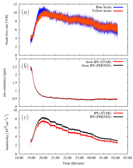
Figure 1: (Color online) U+U store (fill number 16858) with relative beam loss rates (a), normalized rms emittances calculated from luminosity and intensity (b), and luminosities at the STAR and PHENIX experiments (c). The reduction in the emittances and the corresponding increase in the luminosity are due to stochastic cooling during store.

IV Total cross section measurement

For round beams of the same size in both rings the time-dependent luminosity is given by Furm1 ; Furm2

$$\begin{split}\mathcal{L}(t)&=(\beta\gamma)\frac{n_{c}}{T_{rev}}\frac{N_{bB}N_{bY}}{4\pi\varepsilon\beta^{*}}h(\sigma_{s},\beta^{*})\end{split}$$ (3)

where $\gamma$ is the Lorentz factor, and $\gamma^{2}=1/(1-\beta^{2})$, $n_{c}$ is the number of colliding bunches ($n_{c6}=102$ for $\mathcal{L}_{6}$ at STAR, $n_{c8}=111$ for $\mathcal{L}_{8}$ at PHENIX), $T_{rev}$ is the revolution time, $N_{bB},N_{bY}$ are the Blue and Yellow bunch intensities, $\varepsilon=\varepsilon_{x,B}=\varepsilon_{y,B}=\varepsilon_{x,Y}=\varepsilon_{y,Y}$ is the normalized rms emittance, and $\beta^{*}=\beta^{*}_{x,B}=\beta^{*}_{y,B}=\beta^{*}_{x,Y}=\beta^{*}_{y,Y}$ the beam envelope function at the IP. The factor $h(\sigma_{s},\beta^{*})$, $\sigma_{s}$ being the longitudinal rms beam size, is not larger than and of order 1. It captures the hourglass and crossing angle effect. For Gaussian longitudinal distributions $h$ can be calculated Furm1 . In the case of RHIC a numerical integration over the measured longitudinal particle distributions is necessary since the beams are held in two radio frequency systems (harmonic numbers $h=360$ and $h=7\times 360$) and the bunches span several of the higher harmonic buckets at the end of a store.

In the case where all beam losses are given by the total U+U cross section $\sigma_{tot}$ we have

$$\frac{dN_{B}(t)}{dt}=\frac{dN_{Y}(t)}{dt}=-\left[\mathcal{L}_{6}(t)+\mathcal{L}_{8}(t)\right]\sigma_{tot}$$ (4)

where $N_{B}$ and $N_{Y}$ are the Blue and Yellow beam total intensities, and $\mathcal{L}_{6}(t)$ and $\mathcal{L}_{8}(t)$ the instantaneous luminosities at IP6 (STAR) and IP8 (PHENIX) respectively. The total cross section is then given by

$$\sigma_{tot}=-\frac{\dot{N}_{B,Y}(t)}{\left[\mathcal{L}_{6}(t)+\mathcal{L}_{8}(t)\right]}$$ (5)

and the systematic relative error by

$$\frac{\Delta\sigma^{sys}}{\sigma_{tot}}=\frac{\Delta\dot{N}_{B,Y}^{sys}}{\dot{N}_{B,Y}}+\frac{\Delta\mathcal{L}_{6}^{sys}+\Delta\mathcal{L}_{8}^{sys}}{\mathcal{L}_{6}+\mathcal{L}_{8}}$$ (6)

where $\Delta\dot{N}_{B,Y}^{sys}$ and $\Delta\mathcal{L}_{6,8}^{sys}$ are the systematic errors of the beam loss rate and luminosity, respectively. If timing errors can be neglected (see Sec. IV.3) we can use

$$\frac{\Delta\dot{N}_{B,Y}^{sys}}{\dot{N}_{B,Y}}=\frac{\Delta N_{B,Y}^{sys}}{N_{B,Y}}$$ (7)

and the systematic error becomes

$$\Delta\sigma^{sys}=\sigma_{tot}\left(\frac{\Delta N_{B,Y}^{sys}}{N_{B,Y}}+\frac{\Delta\mathcal{L}_{6}^{sys}+\Delta\mathcal{L}_{8}^{sys}}{\mathcal{L}_{6}+\mathcal{L}_{8}}\right).$$ (8)

We also note that if all beam losses are due to burn-off, both the transverse and longitudinal emittances are constant, and all bunches collide at IP6 and IP8 (i.e. $n_{c6}=n_{c8}=n_{c}$), the intensities and luminosities can be written as

$$N_{B,Y}(t)=\frac{N_{B,Y}(0)}{1+t/\tau}\;\;\;\mathrm{and}\;\;\;\mathcal{L}_{6,8}(t)=\frac{\mathcal{L}_{6,8}(0)}{(1+t/\tau)^{2}}$$ (9)

where the time constant $\tau$ follows from Eq. (4) as

$$\tau=\frac{N_{B,Y}(0)}{\left[\mathcal{L}_{6}(0)+\mathcal{L}_{8}(0)\right]\sigma_{tot}}.$$ (10)

We need to obtain the beam loss rates $\dot{N}_{B,Y}$ and the luminosities $\mathcal{L}_{6,8}$ for the determination of the total cross section $\sigma_{tot}$ via Eq. (5). The beam loss rate is calculated from a time-dependent measurement of the total beam intensity with a Parametric Current Transformer (PCT, Appendix B). The total intensity is reported every second and the loss rate is calculated as the slope over an interval of 20 s. The luminosity is measured via the detection of neutron pairs in time-coincidence in the Zero Degree Calorimeter (ZDC) ZDC2 (Appendix C). The luminosity is also reported every second.

IV.1 Luminous and non-luminous losses

A principal limitation of the method used here comes from the fact that there can be beam losses from other processes than U+U interactions given by the total cross section $\sigma_{tot}$. In a situation with non-luminous losses, the use of equation (5) will only give an upper limit for $\sigma_{tot}$ if these non-luminous losses are not subtracted.

A number of tests are available to assess if there are non-luminous losses:

1. The Blue and Yellow beam loss rates $\dot{N}_{B,Y}$ must be the same if all losses are luminous.

2. The Blue and Yellow beam loss rates $\dot{N}_{B,Y}$ must be proportional to the total luminosity $\mathcal{L}_{6}+\mathcal{L}_{8}$.

3. The beam loss rates $\dot{N}_{B,Y}$ must be zero for non-colliding beams.

These are necessary but not sufficient conditions for all beam losses to be luminous. We will use conditions 1 and 2 later to guide the data selection but we have no direct experimental data to test condition 3.

There are a number of processes that can lead to non-luminous beam losses:

1. Intrabeam scattering

2. Residual gas elastic scattering

3. Dynamic aperture and beam-beam effects

4. Residual gas inelastic scattering

In our discussion we need to separate emittance growth processes from beam loss processes. Emittance growth will eventually lead to beam loss once a limiting aperture is reached by the particles with the largest amplitudes. With stochastic cooling the emittance growth is reversed and an equilibrium emittance is reached for processes with growth times comparable to or smaller than the cooling time of about 1 h. Items 1-3 of the above list fall in this category.

In some processes the particle amplitudes can be increased much faster than the cooling time. Item 3 can and item 4 does fall in this category. These processes are discussed in detail in Appendix A and summarized in Tab. 3. We must expect that there are a small number of particles lost through other processes than burn-off, and our analysis of the experimental data needs to take this into account. The predominant process is inelastic scattering on the residual gas, leading to beam loss rates of which are about 10% of the total loss rate at the beginning of the store, and 3% at the time of $\mathcal{L}_{max}$ (see Tab. 3 and Fig. 2).

Table 3: Emittance growth and non-luminous beam loss for U+U collisions in RHIC with beam parameters given in Tab. 2. Formulas are given in Appendix A. The values are shown for either the beginning of store or the time of $\mathcal{L}_{max}$, whichever gives the larger emittance growth or beam loss. The emittance growth times are calculated in the absence of cooling; cooling times are of order 1 h. Only the warm regions of the vacuum system are considered in the calculation of residual gas effects. The cold regions with cryo pumping have very low particle densities.

parameter	unit	value
warm vacuum sections
length per ring $l_{w}$	m	652
gas temperature	K	300
average pressure $\langle P\rangle$	nTorr	0.5
static gas composition	…	95% H2, 5% CO
average $\beta$-functions $\langle\beta\rangle$	m	115
emittance growth from intrabeam scattering
transverse emittance growth time $\tau_{\varepsilon_{n}}$	h	0.44
longitudinal emittance growth time $\tau_{\varepsilon_{s}}$	h	0.55
transverse emittance growth from residual gas elastic scattering
emittance growth coefficient for N2	s-1Torr-1	0.88
N2 equivalent pressure	nTorr	0.5
emittance growth time $\tau_{\varepsilon_{n}}$, at $\mathcal{L}_{max}$	h	49
beam loss from residual gas inelastic scattering
coefficient for beam loss on N2	s-1Torr-1	800
N2 equivalent pressure	nTorr	0.1
beam lifetime $\tau_{N}=N_{B,Y}/\dot{N}_{B,Y}$	h	498
loss rate $\dot{N}_{B,Y}$, initial	1000 s-1	19

IV.2 Measurement value and statistical error

There were 60 physics U+U stores with an average length of 6.4 h (Tab. 4). As a first step we selected all stores which did not have any unusually high beam losses, and in which the Blue and Yellow beam loss rates $\dot{N}_{B}$ and $\dot{N}_{Y}$ were approximately equal and proportional to the total luminosity $\mathcal{L}_{6}+\mathcal{L}_{8}$ for at least a period of the store. These were the last 50 of all 60 physics stores.

Table 4: U+U store overview for $\sigma_{tot}$ determination.

parameter	unit	value
no of physics stores	…	60
average store length	h	6.4
no of stores selected with $\dot{N}_{B}$ data	…	8
no of stores selected with $\dot{N}_{Y}$ data	…	20
total number of data points $(\dot{N},\mathcal{L})$	…	554k

For each of these stores a fitted value for $\sigma_{tot}$ was obtained by assuming that all losses are luminous, i.e. by fitting a straight line to all pairs $(\dot{N},\mathcal{L})$ imposing the condition of a zero offset. The fits for one store are shown in Fig. 2, and the caption notes the standard statistical error for the fit.

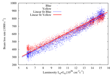
Figure 2: (Color online) Blue and Yellow beam loss rates as a function of the total luminosity $\mathcal{L}_{6}+\mathcal{L}_{8}$ for fill number 16858. The units for the luminosity and beam loss rates are chosen so that the linear fit coefficient is returned in units of barn. Fitted values for this case are $\sigma_{tot}=(516.53\pm 0.21)$ barn for Blue, and $\sigma_{tot}=(549.61\pm 0.16)$ barn for Yellow. The error is the statistical standard error.

Figure 3 shows the so fitted $\sigma_{tot}$ values for all pre-selected stores. The earlier stores (fill numbers 16796 to 16817) show a much larger fitted $\sigma_{tot}$ value than the later stores, indicating that not all beam losses were luminous. We note that all pre-selected stores have longitudinal stochastic cooling, and that transverse stochastic cooling became available in the Yellow ring beginning with fill number 16816, and in the Blue ring with fill number 16820, initially in the vertical plane only. Beginning with fill number 16832 in the Yellow ring and 16835 in the Blue ring the beams were cooled in all three dimensions. We further restrict our data selections to fill number 16820 and larger. But even for those fills we cannot be sure that all losses are luminous. Indications of this are the differences in the fitted $\sigma_{tot}$ from the Blue and Yellow beam in the same store, and variations across stores.

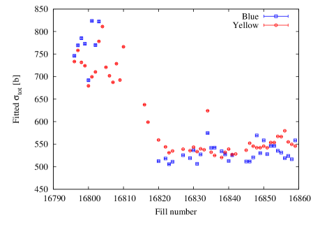
Figure 3: (Color online) Fitted $\sigma_{tot}$ for all (partial) stores during which the beam loss rate was proportional to the total luminosity $\mathcal{L}_{6}+\mathcal{L}_{8}$. All fills shown have longitudinal cooling. Vertical cooling started in Yellow with fill 16816, and in Blue with fill 16820. Horizontal cooling started in Yellow with fill 16832, and in Blue with fill 16835. In fill 16834 a cavity tripped leading to an increase in the momentum spread.

In a second step we fit $\sigma_{tot}$ to the $(\dot{N},\mathcal{L})$ data points for all stores with fill number 16820 and larger under the assumption that there are residual beam losses, i.e. with a nonzero offset. In Fig. 4 we show the fitted values for both $\sigma_{tot}$ and the residual beam loss rates, where we restricted the data selection to data points with a residual beam loss rate not larger than 30000 s^-1, about 10% of the minimum and 3% of the maximum beam loss rates observed (see Fig. 2), to ensure that the $\sigma_{tot}$ determination is done with conditions of nearly all beam losses due to burn-off.

Combining the individual data points in Fig. 4 yields the measurement value and statistical error as $\sigma_{tot}=(515\pm 13^{stat})$ barn. We have calculated the statistical error simply as the standard deviation of the $\sigma_{tot}$ distribution since this distribution is much wider than the statistical errors for the individual data points.

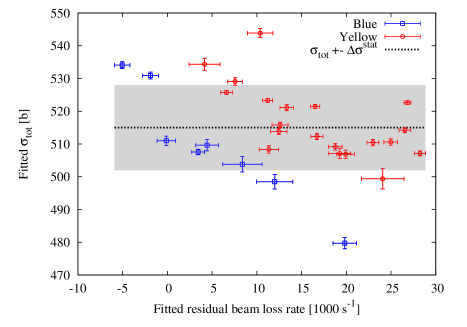
Figure 4: (Color online) Fitted $\sigma_{tot}$ and fitted residual beam loss rates for selected stores. The errors of the individual data points are the standard errors from the linear fit. Shown is also the average of the $\sigma_{tot}$ values and the rms error of the combined individual data points as the gray area, giving $\sigma_{tot}=(515\pm 13^{stat})$ barn.

IV.3 Measurement systematic error

If timing errors can be neglected, the systematic error is given by Eq. (8). We will now justify this assumption. The RHIC timing system is driven by a 5 MHz ultra-low noise temperature-controlled crystal oscillator with a relative frequency error of $\pm 10^{-9}$ to $\pm 10^{-10}$ per day Wenz . However, the timing error of reported 1 Hz signals, such as intensity and luminosity, have a much larger error. The combined systematic, periodic (due to clock beating), and random timing error can reach values of 1 s, but typically does not exceed 0.5 s. Periodic and random errors with a symmetric distribution around a central value will only translate into statistical errors of the fitted total cross section (see Fig. 2), which we have taken into account already.

Using the data shown in Figs. 1 and 2, a systematic timing error of 0.5 s is equivalent to a maximum systematic relative beam loss error of $(\Delta\dot{N}_{B,Y}/N_{B,Y})^{sys}_{max}=3.8\times 10^{-5}$ and a maximum systematic relative luminosity error of $(\Delta\mathcal{L}_{6,8}/\mathcal{L}_{6,8})^{sys}_{max}=3.3\times 10^{-5}$. These are much smaller than other systematic errors for the beam loss rate and luminosity respectively (see below), and we therefore neglect timing errors.

The systematic error $\sigma^{sys}$ is then determined by the systematic errors of the beam intensity and luminosities. These are discussed in detail in Appendix B and Appendix C respectively. The sources and contributions of all components are summarized in Tab. 5 and Tab. 6, and, using Eq. (8) we obtain $\sigma^{sys}=22$ barn.

Table 5: Sources and contributions to the systematic errors in the beam intensity $\Delta N_{B,Y}^{sys}/N_{B,Y}$ (Appendix B).

source	error
temperature variations	0.19%
bunch pattern	0.10%
calibration error	0.15%
PCT accuracy and readout drifts	0.30%
output noise	0.01%
total $\Delta N_{B,Y}^{sys}/N_{B,Y}$ (quadratic addition)	0.40%

Table 6: Sources and contributions to the systematic errors in the luminosity $\Delta\mathcal{L}^{sys}/\mathcal{L}$ (Appendix C and Ref. Dree ).

source	error
beam displacement	1.0%
crossing angle	2.0%
intensity	2.7%
statistical	1.7%
total $\Delta\mathcal{L}^{sys}/\mathcal{L}$ (quadratic addition)	3.9%

V Summary

In U+U stores at $\sqrt{s_{NN}}=192.8$ GeV with 3D stochastic cooling nearly all beam losses are from burn-off and the total interaction cross section can be obtained from the observed beam loss rates as

$$\sigma_{tot}^{meas}=(515\pm 13^{stat}\pm 22^{sys})\;\text{barn}$$ (11)

with a combined statistical and systematic measurement error of 26 barn or 5.0%. The principal limitation of the measurement method are non-luminous beam losses that are not accounted for. If these exist the measurement only delivers an upper limit for $\sigma_{tot}^{meas}$. The calculated total cross section of $\sigma_{tot}^{calc}=487.3\;\text{barn}$ is smaller than the measured one by 28 barn or 5.4%, a value close to the combined measurement error.

VI Acknowledgments

The authors are thankful for discussions and support to J. Bergoz, S. Binello, R. Bruce, W. Christie, T. Hayes, X. He, M. Mapes, A. Marusic, K. Smith, and J. Jowett. Work supported by Brookhaven Science Associates, LLC under Contract No. DE-AC02-98CH10886 with the U.S. Department of Energy.

Appendix A Non-Luminous beam losses

A.1 Intrabeam scattering

Intrabeam scattering refers to small changes in the momenta of stored particles due to close encounters with other stored particles, leading to emittance growth piw1 . In our case intrabeam scattering is counteracted by stochastic cooling, leading to a reduction of the emittance until an equilibrium value is reached.

Table 3 shows the emittance growth times

$$\tau_{\varepsilon}=\left(\frac{1}{\varepsilon}\frac{d\varepsilon}{dt}\right)^{-1}$$ (12)

in the absence of cooling for the transverse and longitudinal planes. Consistent with operational experience full transverse coupling is assumed and therefore the horizontal and vertical growth rates are equal. The calculation is for the time when $\mathcal{L}_{max}$ is reached and the emittances are close to their minimum value (Fig. 1).

We also estimate the lifetime of uranium beams due to intrabeam scattering in the presence of cooling. The emittance evolution is shown in Fig. 1 where the asymptotic cooling time is about 1 h. The collimator settings correspond to an rms emittance of $80~{}\mu$rad, and the simplest model is to assume the emittance distribution follows

$$\frac{\partial w(\varepsilon,t)}{\displaystyle\partial t}={\partial\over\partial\varepsilon}\left(a\varepsilon w+M\varepsilon{\partial w\over\displaystyle\partial\varepsilon}\right),$$ (13)

where $w(\varepsilon,t)$ is the time-dependent emittance distribution, $a$ is the cooling rate and $M$ is the diffusion rate. We have $a=1~{}{\rm h}^{-1}$ and $\varepsilon_{a}=M/a=0.5~{}{\mu}$rad. If we put a collimator (an element that ensures particle removal when a certain amplitude is exceeded) at a location equivalent to an emittance of $\varepsilon_{b}=80~{}{\mu}$rad the beam lifetime will be piw1

$$\tau_{N}=\frac{\varepsilon_{a}}{a\varepsilon_{b}}\exp\left(\frac{\varepsilon_{b}}{\varepsilon_{a}}\right)\sim 10^{67}{\rm h}.$$ (14)

Beam losses from intrabeam scattering with cooling can indeed be neglected.

A.2 Residual gas elastic scattering

We consider only the warm sections of RHIC since the residual gas density in the cold arcs is very low due to cryo pumping. The rms emittance growth time due to residual gas elastic scattering is Mokh ; Syph

$$\frac{1}{\tau_{\varepsilon_{n}}}=\frac{Z}{A}\frac{1}{\varepsilon_{n}}\frac{d\varepsilon_{n}}{dt}=\frac{(\beta\gamma)}{\varepsilon_{n}}\times\frac{1}{C}\int_{0}^{C}\beta(s)\theta_{rg}^{2}(s)ds$$ (15)

where $Z$ and $A$ are the charge and mass number of the stored ion, $C$ is the circumference and $\theta_{rg}$ the rms scattering angle. For protons, scattering on species with atomic number $Z_{i}$ and density $n_{i}$, the scattering angle is Mokh

$$\theta_{rg}^{2}(s)=\frac{4\pi r_{p}^{2}c}{\beta^{3}\gamma^{2}}n_{i}Z_{i}(Z_{i}+1)\ln(183Z_{i}^{-1/3}),$$ (16)

where $r_{p}$ is the classical proton radius and $c$ the speed of light. For molecular nitrogen N₂ at 300 K one has

$$\frac{1}{\tau_{\varepsilon_{n}}}\approx 0.88\,\mathrm{s}^{-1}\mathrm{Torr}^{-1}\frac{l_{w}}{C}\frac{\langle\beta P\rangle}{\varepsilon_{n}\gamma}.$$ (17)

where $l_{w}$ is the length of the warm sections. For other residual gas species the N₂ equivalent pressure can be calculated according to Ref. Mokh as

$$\begin{split}P_{N_{2}equiv}^{elast}&=\frac{2\times 10^{-3}}{P}\times\\ &\phantom{=}\sum_{i}P_{i}\sum_{j}k_{ij}Z_{ij}(Z_{ij}+1)\ln(183Z_{ij}^{-1/3}),\end{split}$$ (18)

where $P_{i}$ is the partial pressure of gas molecules $i$, and $k_{ij}$ the number of species $j$ in the gas molecule $i$. Average $\beta$-functions of the warm sections and calculated emittance growth times are shown in Tab. 3.

A.3 Residual gas inelastic scattering

Stored beam particles are lost after an inelastic collision with molecules of the residual gas in the beam pipe. The beam loss rate due to residual gas inelastic scattering of ions on molecular nitrogen N₂ at 300 K is Fisc2 ; Mokh

$$-\frac{dN_{B,Y}}{dt}\approx 800\,\mathrm{s}^{-1}\mathrm{Torr}^{-1}A^{2/3}N_{B,Y}\frac{\langle\beta\rangle}{C}\int_{0}^{C}P(s)ds,$$ (19)

where $\langle\beta\rangle$ is the average $\beta$-function, $C$ the circumference, and $P(s)$ the $s$-dependent N₂ pressure. The nitrogen equivalent pressure can be calculated as Mokh

$$P_{N_{2}eqiv}^{nucl}=0.0861\sum_{i}P_{i}\sum_{j}k_{ij}A_{ij}^{2/3}$$ (20)

where $P_{i}$ is the partial pressure of gas molecules $i$, $k_{ij}$ are the number of species $j$ in the gas molecule $i$, and $A_{ij}$ the mass number of species $j$ in molecule $i$. We consider only the warm beam pipe regions, and neglect the cryogenically pumped cold beam pipe regions. The relevant input data and calculated loss rate are shown in Tab. 3. The calculated loss rate is for the beginning of the store and has an error of approximately a factor of two, primarily due to the uncertainty in the pressure readings. The beam loss rate due to inelastic scattering decreases throughout the store with the decrease of the number of stored particles.

A.4 Dynamic aperture and beam-beam effects

Orbit, tune, and chromaticity settings are chosen to minimize non-luminous beam losses. However, actual machine conditions are not always reproducible, and can drift with time, due to e.g. temperature changes. Beam losses are monitored continuously during stores, and small parameter changes are periodically made to ensure that the machine operates at the minimum achievable loss rates. We disregard time-periods with beam loss rates higher than the consistently low values established over a number of stores.

The motion of hadrons stored in a collider ring is well approximated by Hamiltonian mechanics (non-Hamiltonian effects were discussed above). The particle motion in storage rings can be and typically is chaotic, which leads to emittance growth and possibly particle loss over the storage time Seid ; Seid1 ; Mess ; Fisc3 . In addition to nonlinear elements such as sextupoles, magnetic field errors in the main dipoles and quadrupoles, and the beam-beam interactions, there are parameter modulations that cause or enhance chaotic motion.

Emittance growth effects due to nonlinear elements and parameter modulations are generally smaller than the cooling time and will not lead to any relevant losses (see Sec. A.1). Chaotic particles can also be lost over much smaller time scales than the cooling time Fisc3 . But with cooling particles remain at small amplitudes, far away from the dynamic aperture, and this is much less likely.

Appendix B Intensity measurement and systematic intensity error

The instruments to measure the number of ions present in each RHIC ring are two Bergoz Parametric Current Transformers (PCTs) Berg . These devices often referred to as DC Current Transformers (DCCTs) are sophisticated refinements of the basic fluxgate magnetometer Evan invented in the 1930s by Victor Vacquier at Gulf Research Laboratories, and used in World War II to detect the proximity of submarines. The version now widely used for accelerator beam instrumentation was invented in 1969 by K.B. Unser at CERN Unse and further refined by J. Bergoz Berg and his collaborators. The PCTs measure all ions circulating, bunched and unbunched. The unbunched beam is never more than a few percent of the total intensity, and since it is distributed over the full circumference, its density is very low. It therefore does not contribute measurably to the luminosity.

It is important to note that this is a zero-crossing device in which the fluxes induced by the beam in very high permeability cores is compensated in a closed feedback loop by a current in windings that produce the opposite fluxes. In addition there are other windings that modulate the fluxes, causing the cores to cross from saturation in one direction to saturation in the opposite direction. These transitions are detected by pickup coils and the lack of symmetry (i.e. the presence of odd harmonics) of these signals is used as the error signal to close the feedback loop. The large dynamic range of these instruments (of order $10^{7}$) is mainly due to the fact that the flux in the cores is near zero no matter what the value is of the measured field. This also means that most measurement errors (except for noise) are only weakly intensity dependent.

Rather than using the internal PCT instrument calibration, we use a precise external current source Keith1 and digitize the output in a high precision Digital Volt Meter (DVM) Keith2 . Both of these instruments are calibrated annually.

The PCT calibration software in LabVIEW determines offset and slope values for the DVM readings as function of calibration current for both PCTs. These values are then used to correct the readings and to arrive at values for the number of ions in each ring by taking into account their charge states and their revolution frequency. PCT calibrations are performed before each running period.

One issue investigated before starting the error evaluation was the placement of the coil used to inject the calibration current. The concern was that its different geometry compared to the beam may lead to a correction factor that may not have been considered. In fact, some facilities Dena use straight calibration wires parallel to the beam. It was determined that this is not an issue both experimentally and by consultation with experts Blas ; Berg1 . In the following we discuss one by one the sources of error that contribute to the overall uncertainty in the beam intensity determinations.

B.1 Temperature variations

According to the PCT User Manual the temperature coefficient for the electronics is $<0.1$ $\mu$A/K for the electronics but it is typically 5 $\mu$A/K for the sensor head. There is no temperature regulation in the system nor are there corrections applied, even though the core temperatures are recorded. Figure 5 shows the temperature of the Blue and Yellow PCTs from October 2011 to July 2012. The maximum variation is 5K.

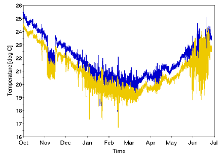
Figure 5: (Color online) Blue and Yellow ring PCT core temperatures from October 2011 to June 2012, covering the period of the 2012 RHIC run.

Since the PCT calibration used is the one performed just before the 2012 running period when the temperature was highest, and the uranium operation took place from 19 April to 15 May 2012, we use the full 5K excursion resulting in a current error due to temperature of 5 $\mu$A/K $\times$ 5 K $=25$ $\mu$A. This translates into an intensity error of 0.19% (Tab. 5).

B.2 Bunch pattern influence

The variation of the PCT output signal as a function of the bunch pattern, or duty factor, was measured by connecting a variable duty factor DC current supply to the calibration windings (Fig. 6). This measurement shows that the fill pattern contributes less than 0.10% to the systematic intensity error (Tab. 5).

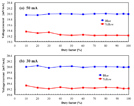
Figure 6: (Color online) Measurement of the variation of the PCT output signal as a function of duty factor.

B.3 Calibration instrument errors

Table 7 shows examples for particular ranges for the accuracy in parts per million (ppm) of full scale for the DVM and the Current source that are used for the PCT calibrations.

We see that the only possibly relevant contribution to the error comes from the current source. It is 0.15% of full scale if we add the drift over one year to the effect of a 5 K temperature uncertainty. This number can be refined to take into account the use of other ranges and of currents that are not full-scale. Calibration errors yield an intensity error of 0.15% (Tab. 5).

Table 7: Accuracy and temperature coefficients of current calibration instruments Keith1 ; Keith2 .

instrument	range	24 h	90 d	1 y	temperature
					coefficient
		[ppm]	[ppm]	[ppm]	[ppm/K]
Keithley 2000	10 V	15	20	30	2
Keithley 220	100 mA			100,000	10,000

B.4 Zero and slope drift

The PCT calibration is typically performed at the beginning of the running period and the question is by how much the calibration parameters can vary during the run. We have already considered the temperature effect above. Here we list other sources of errors that can affect the calibration taken from the specifications found in the PCT user manual:

• Linearity error $\pm 0.01$% $\pm$ zero error

• Zero drift (1 hour) $<1$ $\mu$A

• Zero drift (1 year) $<5$ $\mu$A at constant temperature

• Absolute accuracy $>\pm 0.1$%

We have compared some of these values with slope values for two instances where calibration parameters before and after a calibration were logged and one where calibrations were logged two days apart.

We see that all the slope differences between calibrations are largest for the MADC measurements which vary by an average of 0.14% when the measurements are months apart and 0.036% when they are 2 days apart. The DVM measurements are much better than could be expected from the current source specifications. Independent of the digitizer used the slope values always repeat within 0.2%.

B.5 Noise contributions

In the past, some discrepancies were observed when comparing expected DVM readings with actual readings obtained with a series of current source settings. These discrepancies were attributed to noise. Such measurements were repeated. Figure 7 shows the differences between expected and observed values and the quality of linear least square fit indicates that the discrepancies are mainly due to a calibration issue which is compensated for in the calibration procedure.

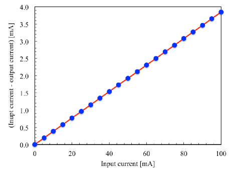
Figure 7: (Color online) Difference between expected and observed DVM readings. The rms deviation from a straight line is 2.4 $\mu$A, not visible in this plot.

The error sources and values are summarized in Tab. 5. For those errors that were obtained in units of current, such as the temperature correction, the values were converted to percentages by using an average beam current of 28 mA, typical for the uranium beams mid-store in the experiments (Tab. 2 shows the values at the beginning of the store and at the time of the maximum luminosity). Output noise contributes only 0.01% to the systematic intensity error (Tab. 5).

Appendix C Luminosity measurement and systematic luminosity error

The luminosity is measured via the detection of neutron-pair coincidences in the Zero Degree Calorimeter (ZDC) ZDC0 ; ZDC2 . The effective cross section for neutron-pair coincidence detection was measured to be $\sigma_{nn}=15.79$ barn for PHENIX, and $\sigma_{nn}=15.84$ barn for STAR. These values are in good agreement with the calculated cross sections given in Tab. 1. Indeed, by accounting for the fact that about 97% of the EMD events are accompanied by the emission of at least one neutron at each side, the value of 15.34 b is obtained as $(0.97\times 0.97\times 7.59+8.2)$ b, providing that forward neutrons are always emitted in nuclear collisions.

A general outline of the error analysis of luminosity measurements is given in Ref. Whit , and the detailed analysis of the U+U luminosity error in Ref. Dree . The following effects were considered in the determination of the luminosity error: (i) the need for a double Gaussian fit function for the luminosity as a function of relative beam offset, (ii) the total intensity measurement, (iii) the bunched intensity measurement, (iv) the fill pattern, (v) the relative position measurement error, (vi) the crossing angle. A summary of the error sources and contributions is provided in Tab. 6.

References

- (1) H. Gould, Lawrence Berkeley Laboratory Report No. LBL-18593 (1984).
- (2) A.J. Baltz, M.-J. Rhoades-Brown, and J. Wesener, Phys. Rev. E 54, 4233 (1996).
- (3) S.R. Klein, Nucl. Instrum. Methods Phys. Res., Sect. A 459, 51 (2001).
- (4) J.M. Jowett, J.-B. Jeanneret, and K. Schindl, Proceedings of the Particle Accelerator Conference 2003, Portland, Oregon, pp. 1682-1684 (2003).
- (5) R. Bruce, J.M. Jowett, S. Gilardoni, A. Drees, W. Fischer, S. Tepikian, and S.R. Klein, Phys. Rev. Lett. 99, 144801 (2007).
- (6) K.H. Ackermann et al. (STAR collaboration), Phys. Rev. Lett. 86 (2001), pp. 402.
- (7) Y. Luo, J. Alessi, M. Bai, E. Beebe, J. Beebe-Wang, I. Blackler, M. Blaskiewicz, J.M. Brennan, K.A. Brown, D. Bruno, J. Butler, R. Connolly, T. D’Ottavio, K.A. Drees, A.V. Fedotov, W. Fischer, C.J. Gardner, D.M. Gassner, X. Gu, Y. Hao, M. Harvey, T. Hayes, L.T. Hoff, H. Huang, P. Ingrassia, J. Jamilkowski, N.A. Kling, M. Lafky, J.S. Laster, C. Liu, D. Maffei, Y. Makdisi, M. Mapes, G.J. Marr, A. Marusic, F. Meot, K. Mernick, R. Michnoff, M. Minty, C. Montag, J. Morris, C. Naylor, S. Nemesure, A.I. Pikin, P. Pile, V. Ptitsyn, D. Raparia, G. Robert-Demolaize, T. Roser, P.W. Sampson, J. Sandberg, V. Schoefer, C. Schultheiss, F. Severino, T. Shrey, K. Smith, S. Tepikian, P. Thieberger, D. Trbojevic, J. Tuozzolo, B. Van Kuik, G. Wang, M. Wilinski, A. Zaltsman, K. Zeno, S.Y. Zhang, and W. Zhang, proceedings of the International Particle Accelerator Conference 2013, Shanghai, China, pp. 1538-1540 (2013).
- (8) Y. Luo, M. Blaskiewicz, W. Fischer, X. Gu, and S. Tepikian, proceeding of the International Particle Accelerator Conference 2012, New Orleans, Louisiana, pp. 175-177 (2012).
- (9) M. Blaskiewicz and J.M. Brennan, Phys. Rev. ST + Accel. Beams 10, 061001 (2007).
- (10) M. Blaskiewicz, J.M. Brennan, and F. Severino, Phys. Rev. Lett. 100, 174802 (2008).
- (11) M. Blaskiewicz, J.M. Brennan, and K. Mernick, Phys. Rev. Lett. 105, 094801 (2010).
- (12) G. Racah, Nuovo Cimento 14,93 (1937).
- (13) L. D. Landau and E. M. Lifshitz, Phys. Z. Sowjetunion 6, 244 (1934).
- (14) H. Meier, Z. Halabuka, K. Hencken, D. Trautman, and G. Baur, Phys. Rev. A, Vol. 63, 032713 (2001).
- (15) A. J. Baltz, Phys. Rev. Lett. 78, 1231 (1997).
- (16) A.J. Baltz, C. Chasman, and S.N. White, Nucl. Instrum. and Methods A 417, pp. 1-8 (1998).
- (17) A.J. Baltz, G. Baur, D. d’Enterria, L. Frankfurt, F. Gelis, V. Guzey, K. Hencken, Yu. Kharlov, M. Klasen, S.R. Klein, V. Nikulin, J. Nystrand, I.A. Pshenichnov, S. Sadovsky, E. Scapparone, J. Seger, M. Strikman, M. Tverskoy, R. Vogt, S.N. White, Phys. Reports 458, 1 (2008).
- (18) I.A. Pshenichnov, Phys. Part. Nuclei 42, 215 (2011).
- (19) C. Oppedisano, J. Phys. G 38, 124174 (2011).
- (20) B. Abelev et al., ALICE collaboration, B. Abelev et al., ALICE collaboration, Phys. Rev. Lett. 109, 252302 (2012).
- (21) I.A. Pshenichnov, J.P. Bondorf, I.N. Mishustin, A. Ventura, and S. Masetti, Phys. Rev. C, Vol. 64, 024903 (2001).
- (22) M. L. Miller, K. Reygers, S. J. Sanders, and P. Steinberg, Ann. Rev. Nucl. Part. Sci. 57, 205 (2007)
- (23) C. Scheidenberger, I. A. Pshenichnov, K. Summerer, A. Ventura, J. P. Bondorf, A. S. Botvina, I. N. Mishustin, and D. Boutin et al., Phys. Rev. C 70, 014902 (2004).
- (24) G. Antchev, P. Aspell, I. Atanassov, V. Avati, J. Baechler, V. Berardi, M. Berretti, and E. Bossini et al., Europhys. Lett. 96, 21002 (2011)
- (25) M. Harrison, T. Ludlam, and S. Ozaki, Nucl. Instrum. and Methods A 499, pp. 235-244 (2003).
- (26) W. Fischer, proceeding International Particle Conference 2010, Kyoto, Japan, pp. 1227-1231 (2010).
- (27) J.G. Alessi, E.N. Beebe, S. Binello, C.J. Gardner, O. Gould, L.T. Hoff, N.A. Kling, R.F. Lambiase, V. LoDestro, R. Lockey, M. Mapes, A. McNerney, J. Morris, M. Okamura, A. Pendzick, D. Phillips, A.I. Pikin, D. Raparia, J. Ritter, T.C. Shrey, L. Smart, L. Snydstrup, C. Theisen, M. Wilinski, A. Zaltsman, K. Zeno, U. Ratzinger, and A. Schempp, proceedings Particle Accelerator Conference 2011, New York, USA, pp. 1966-1968 (2011).
- (28) A. Piwinski, “Touschek effect and intrabeam scattering”, in “Handbook of accelerator physics and engineering” edited by A.W. Chao and M. Tigner, World Scientific (1999).
- (29) M.A. Furman and M.S. Zisman, “Luminosity”, in “Handbook of accelerator physics and engineering”, (A.W. Chao and M. Tigner eds.), World Scientific (1999).
- (30) M.A. Furman, “Hourglass effect for asymmetric colliders”, proceedings of the Particle Accelerator Conference 1991, San Francisco, USA, pp. 422-424 (1991).
- (31) C. Adler, A. Denisov, E. Garcia, M. Murray, H. Strobele, and S. White, Nucl. Instrum. and Methods A 470, pp. 488-499 (2001).
-
(32)
Wenzel HF Ultra Low Noise OCXO,
www.wenzel.com - (33) A. Piwinski, CERN 85-19, pp. 432 (1985).
- (34) N.V. Mokhov and V.I. Balbekov, “Beam and luminosity lifetime”, in “Handbook of accelerator physics and engineering”, World Scientific, (1998).
- (35) M. Syphers, “Emittance dilution effects [1]”, in “Handbook of accelerator physics and engineering”, World Scientific, (1998).
- (36) W. Fischer, M. Bai, and P. Harvey, BNL C-A/AP/235 (206).
- (37) M. Seidel, PhD thesis Hamburg University, DESY HERA 93-04 (1993).
- (38) M. Seidel, “The proton collimation system of HERA”, Ph.D. Thesis, Hamburg U., DESY 94-103 (1994).
- (39) K.-H. Mess and M. Seidel, “Collimators as diagnostics tools in the proton machine of HERA”, Nucl. Instrum. Methods A 351, 279 (1994).
- (40) W. Fischer, M. Giovannozzi and F. Schmidt, Phys. Rev. E, Vol. 55, Number 3, p. 3507 (1997).
- (41) BERGOZ Instrumentation, 01170 Crozet, France, http://www.bergoz.com
-
(42)
K. Evans,
http://www.invasens.co.uk/FluxgateExplained.PDF (2006). - (43) K.B. Unser, IEEE Trans. Nucl. Sci., NS-16, pp. 934-938 (1969).
-
(44)
Keithley 220 Current Source,
http://www.keithley.com/products/searchresults?
q=220&sa.x=29&sa.y=12 -
(45)
Keithley 2000 DMM,
www.keithley.com/data?asset=359 - (46) J.C. Denard, A. Saha, and G. Laveissiere, proceedings of the Particle Accelerator Conference 2001, Chicago, Illinois, pp. 2326-2328 (2001).
- (47) M. Blaskiewicz, private communication (2012).
- (48) J. Bergoz, private communication (2012).
- (49) S. White, Ph.D. thesis, Université Paris-Sud 11, LAL-154, CERN-THESIS-2010-139 (2010).
- (50) A. Drees, BNL C-A/AP/495, BNL-103466-2013-IR, arXiv:1312.6618 [physics.acc-ph] (2013).