Separating a Voronoi Diagram via Local Search

Abstract

Given a set $\mathsf{P}$ of $n$ points in ${\rm I\!R}^{d}$, we show how to insert a set $\mathsf{X}$ of $O\!\left({n^{1-1/d}}\right)$ additional points, such that $\mathsf{P}$ can be broken into two sets $\mathsf{P}_{1}$ and $\mathsf{P}_{2}$, of roughly equal size, such that in the Voronoi diagram $\mathcal{V}\!\left({\mathsf{P}\cup\mathsf{X}}\right)$, the cells of $\mathsf{P}_{1}$ do not touch the cells of $\mathsf{P}_{2}$; that is, $\mathsf{X}$ separates $\mathsf{P}_{1}$ from $\mathsf{P}_{2}$ in the Voronoi diagram (or in the dual Delaunay triangulation). Given such a partition $(\mathsf{P}_{1},\mathsf{P}_{2})$ of $\mathsf{P}$, we present approximation algorithms to compute the minimum size separator realizing this partition.

Finally, we present a simple local search algorithm that is a PTAS for geometric hitting set of fat objects (which can also be used to approximate the optimal Voronoi partition).

1 Introduction

Divide and conquer.

Many algorithms work by partitioning the input into a small number of pieces, of roughly equal size, with little interaction between the different pieces, and then recursing on these pieces. One natural way to compute such partitions for graphs is via the usage of separators.

Separators.

A (vertex) separator of a graph $\mathsf{G}=(\mathsf{V},\mathsf{E})$, informally, is a “small” set $\mathcal{Z}\subseteq\mathsf{V}$ whose removal breaks the graph into two or more connected subgraphs, each of which is of size at most $n/c$, where $c$ is some constant larger than one. As a concrete example, any tree with $n$ vertices has a single vertex, which can be computed in linear time, such that its removal breaks the tree into subtrees, each with at most $n/2$ vertices.

Separators in planar graphs.

In 1977, Lipton and Tarjan [LT77, LT79] proved that any planar graph with $n$ vertices contains a separator of size $O\!\left({\sqrt{n}}\right)$, and it can be computed in linear time. Specifically, there exists a separator of size $O(\sqrt{n})$ that partitions the graph into two disjoint subgraphs each containing at most $2n/3$ vertices.

There has been a substantial amount of work on planar separators in the last four decades, and they are widely used in data-structures and algorithms for planar graphs, including (i) shortest paths [FR06], (ii) distance oracles [SVY09], (iii) max flow [EK13], and (iv) approximation algorithms for TSP [Kle08]. This list is a far cry from being exhaustive, and is a somewhat arbitrary selection of some recent results on the topic.

Planar separators via geometry.

Any planar graph can be realized as a set of interior disjoint disks, where a pair of disks touch each other, if and only if the corresponding vertices have an edge between them. This is known as the circle packing theorem [PA95], sometimes referred to in the literature as Koebe-Andreev-Thurston theorem. Its original proof goes back to Koebe’s work in 1936 [Koe36].

Surprisingly, the existence of a planar separator is an easy consequence of the circle packing theorem. This was proved by Miller et al. [MTTV97], and their proof was recently simplified by Har-Peled [Har11b]. Among other things, Miller et al. showed that given a set of $n$ balls in ${\rm I\!R}^{d}$, such that no point is covered more than $k$ times, the intersection graph of the balls has a separator of size $O\!\left({k^{1/d}n^{1-1/d}}\right)$. This in turn implies that the $k$-nearest neighbor graph of a set of points in ${\rm I\!R}^{d}$, has a small separator [MTTV97, Har11b]. Various extensions of this technique were described by Smith and Wormald [SW98].

Other separators.

Small separators are known to exist for many other families of graphs. These include graphs (i) with bounded tree width [BPTW10], (ii) with bounded genus [GHT84], (iii) that are minor free [AST90], and (iv) that are grids.

(A) (B)

Figure 1.1: (A) A Voronoi partition. (B) A separator realizing it.

Voronoi separators.

In this paper, we are interested in geometric separation in a Voronoi diagram. Voronoi diagrams are fundamental geometric structure, see [AKL13]. Specifically, given a set $\mathsf{P}$ of points in ${\rm I\!R}^{d}$, we are interested in inserting a small set of new points $\mathsf{X}$, such that there is a balanced partition of $\mathsf{P}$ into two sets $\mathsf{P}_{1},\mathsf{P}_{2}$, such that no cell of $\mathsf{P}_{1}$ touches a cell of $\mathsf{P}_{2}$ in the Voronoi diagram $\mathcal{V}\!\left({\mathsf{P}\cup\mathsf{X}}\right)$. Note, that such a set $\mathsf{X}$ also separates $\mathsf{P}_{1}$ and $\mathsf{P}_{2}$ in the Delaunay triangulation of $\mathsf{P}\cup\mathsf{X}$.

Why Voronoi separators are interesting?

Some meshing algorithms rely on computing a Delaunay triangulation of geometric models to get good triangulations that describe solid bodies. Such meshes in turn are fed into numerical solvers to simulate various physical processes. To get good triangulations, one performs a Delaunay refinement that involves inserting new points into the triangulations, to guarantee that the resulting elements are well behaved. Since the underlying geometric models can be quite complicated and these refinement processes can be computationally intensive, it is natural to try and break up the data in a balanced way, and Voronoi separators provide one way to do so.

More generally, small Voronoi separators provide a way to break up a point set in such a way that there is limited interaction between two pieces of the data.

Geometric hitting set.

Given a set of objects in ${\rm I\!R}^{d}$, the problem of finding a small number of points that stab all the objects is an instance of geometric hitting set. There is quite a bit of research on this problem. In particular, the problem is NP-Hard for almost any natural instance, but a polynomial time $(1+{\varepsilon})$-approximation algorithm is known for the case of balls in ${\rm I\!R}^{d}$ [Cha03], where one is allowed to place the stabbing points anywhere. The discrete variant of this problem, where there is a set of allowable locations to place the stabbing points, seems to be significantly harder and only weaker results are known [HL12].

One of the more interesting versions of the geometric hitting set problem, is the art gallery problem, where one is given a simple polygon in the plane, and one has to select a set of points (inside or on the boundary of the polygon) that “see” the whole polygon. While much research has gone into variants of this problem [O’R87], nothing is known as far as an approximation algorithm (for the general problem). The difficulty arises from the underlying set system being infinite, see [EH06] for some efforts in better understanding this problem.

Geometric local search.

Relatively little is known regarding local search methods for geometric approximation problems. Arya et al. [AGK⁺01] gave a local search method for approximating $k$-median clustering by a constant factor, and this was recently simplified by Gupta and Tangwongsan [GT08].

Closer to our settings, Mustafa and Ray [MR09] gave a local search algorithm for the discrete hitting set problem over pseudo disks and $r$-admissible regions in the plane, which yields a PTAS. Chan and Har-Peled [CH12] gave a local search PTAS for the independent set problem over fat objects, and for pseudodisks in the plane. Both works use separators in proving the quality of approximation.

1.1 Our Results

In this paper we give algorithms for the following:

1. Computing a small Voronoi separator. Given a set $\mathsf{P}$ of $n$ points in ${\rm I\!R}^{d}$, we show how to compute, in expected linear time, a balanced Voronoi separator of size $O\!\left({n^{1-1/d}}\right)$. This is described in Section 3. The existence of such a separator was not known before, and our proof is relatively simple and elegant.

   Such a separator can be used to break a large data-set into a small number of chunks, such that each chunk can be handled independently – potentially in parallel on different computers.

2. Exact algorithm for computing the smallest Voronoi separator realizing a given partition. In Section 4, given a partition $(\mathsf{P}_{1},\mathsf{P}_{2})$ of a point set $\mathsf{P}$ in ${\rm I\!R}^{d}$, we describe an algorithm that computes the minimum size Voronoi separator realizing this separation. The running time of the algorithm is $n^{O\left({\mathsf{b}}\right)}$, where $\mathsf{b}$ is the cardinality of the optimal separating sets (the $O$ notation is hiding a constant that depends on $d$).

3. Constant approximation algorithm for the smallest Voronoi separator realizing a given partition. In Section 5.1, we describe how to compute a constant factor approximation to the size of the minimal Voronoi separator for a given partition of a set in ${\rm I\!R}^{d}$. This is the natural extension of the greedy algorithm for geometric hitting set of balls, except that in this case, the set of balls is infinite and is encoded implicitly, which somewhat complicates things.

4. A PTAS for the smallest Voronoi separator realizing a given partition. In Section 5.2, we present a polynomial time approximation scheme to compute a Voronoi separator, realizing a given partition, whose size is a $(1+{\varepsilon})$-approximation to the size of the minimal Voronoi separator for a given partition of a set in ${\rm I\!R}^{d}$. The running time is $n^{O(1/{\varepsilon}^{d})}$.

   Interestingly, the new algorithm provides a PTAS for the geometric hitting set problem (for balls), that unlike previous approaches that worked top-down [Cha03, EJS05], works more in a bottom-up approach. Note, that since our set of balls that needs to be pierced is infinite, and is defined implicitly, it is not obvious a priori how to use the previous algorithms in this case.

   Sketch of algorithm. The new algorithm works by first computing a “dirty” constant approximation hitting set using a greedy approach (this is relatively standard). Somewhat oversimplifying, the algorithm next clusters this large hitting set into tight clusters of size $k=O(1/{\varepsilon}^{d})$ each. It then replaces each such cluster of the weak hitting set, by the optimal hitting set that can pierce the same set of balls, computed by using the exact algorithm – which is “fast” since the number of piercing points is at most $O(1/{\varepsilon}^{d})$. In the end of this process the resulting set of points is the desired hitting set. Namely, the new approximation algorithm reduces the given geometric hitting set instance, into $O(m/k)$ smaller instances where $m$ is the size of the overall optimal hitting set and each of the smaller instances has an optimal hitting set of size $O(k)$.

   For the analysis of this algorithm, we need a strengthened version of the separator theorem. See Theorem 5.2${}_{\text{p\ref{theorem:ball:separator}}}$ for details.

5. Local search PTAS for continuous geometric hitting set problems. An interesting consequence of the new bottom-up PTAS, is that it leads to a simple local search algorithm for geometric hitting set problems for fat objects. Specifically, in Section 6, we show that the algorithm starts with any hitting set (of the given objects) and continues to make local improvements via exchanges of size at most $O\!\left({1/{\varepsilon}^{d}}\right)$, until no such improvement is possible, yielding a PTAS. The analysis of the local search algorithm is subtle requiring to cluster simultaneously the locally optimal solution, and the optimal solution, and matching these clusters to each other.

Significance of Results.

Our separator result provides a new way to perform geometric divide and conquer for Voronoi diagrams (or Delaunay triangulations). The PTAS for the Voronoi partition problem makes progress on a geometric hitting set problem where the ranges to be hit are defined implicitly, and their number is infinite, thus pushing further the envelope of what geometric hitting set problems can be solved efficiently. Our local search algorithm is to our knowledge the first local search algorithm for geometric hitting set – it is simple, easy to implement, and might perform well in practice (this remains to be verified experimentally, naturally). More importantly, it shows that local search algorithms are potentially more widely applicable in geometric settings.

How our results relate to known results?

Our separator result is similar in spirit (but not in details!) to the work of Miller et al. [MTTV97] on a separator for a $k$-ply set of balls – the main difference being that Voronoi cells behave very differently than balls do. Arguably, our proof is significantly simpler and more elegant. Our bottom-up PTAS approach seems to be new, and should be applicable to other problems. Having said that, it seems like the top-down approaches [Cha03, EJS05] potentially can be modified to work in this case, but the low level details seem to be significantly more complicated, and the difficulty in making them work was the main motivation for developing the new approach. The analysis of our local search algorithm seems to be new – in particular, the idea of incrementally clustering in sync optimal and local solutions. Of course, the basic idea of using separators in analyzing local search algorithms appear in the work of Mustafa and Ray [MR09] and Chan and Har-Peled [CH12].

2 Preliminaries

For a point set $\mathsf{P}\subseteq{\rm I\!R}^{d}$, the Voronoi diagram of $\mathsf{P}$, denoted by $\mathcal{V}\!\left({\mathsf{P}}\right)$ is the partition of space into convex cells, where the Voronoi cell of $\mathsf{p}\in\mathsf{P}$ is

$$\mathcal{C}_{\mathsf{P}}\!\left({\mathsf{p}}\right)=\left\{{\mathsf{q}\in{\rm I\!R}^{d}\,\left|\,{\left\|{\mathsf{q}}-{\mathsf{p}}\right\|\leq\mathsf{d}\!\left({\mathsf{q},\mathsf{P}}\right)}\rule[-5.69046pt]{0.0pt}{11.38092pt}\right.}\right\},$$

where $\mathsf{d}\!\left({\mathsf{q},\mathsf{P}}\right)=\min_{\mathsf{s}\in\mathsf{P}}\left\|{\mathsf{q}}-{\mathsf{s}}\right\|$ is the distance of $\mathsf{q}$ to the set $\mathsf{P}$. Voronoi diagrams are a staple topic in Computational Geometry, see [BCKO08], and we include the definitions here for the sake of completeness. In the plane, the Voronoi diagram has linear descriptive complexity. For a point set $\mathsf{P}$, and points $\mathsf{p},\mathsf{q}\in\mathsf{P}$, the geometric loci of all points in ${\rm I\!R}^{d}$ that have both $\mathsf{p}$ and $\mathsf{q}$ as nearest neighbor, is the bisector of $\mathsf{p}$ and $\mathsf{q}$ – it is denoted by $\beta_{\mathsf{p},\mathsf{q}}=\left\{{\mathsf{s}\in{\rm I\!R}^{d}\,\left|\,{\left\|{\mathsf{s}}-{\mathsf{p}}\right\|=\left\|{\mathsf{s}}-{\mathsf{q}}\right\|=\mathsf{d}\!\left({\mathsf{s},\mathsf{P}}\right)}\rule[-5.69046pt]{0.0pt}{11.38092pt}\right.}\right\}$. A point $\mathsf{s}\in\beta_{\mathsf{p},\mathsf{q}}$ is the center of a ball whose interior does not contain any point of $\mathsf{P}$ and that has $\mathsf{p}$ and $\mathsf{q}$ on its boundary. The set of all such balls induced by $\beta_{\mathsf{p},\mathsf{q}}$ is the pencil of $\mathsf{p}$ and $\mathsf{q}$, denoted by $\mathrm{pencil}\!\left({\mathsf{p},\mathsf{q}}\right)$.

Definition 2.1.

Let $\mathsf{P}$ be a set of points in ${\rm I\!R}^{d}$, and $\mathsf{P}_{1}$ and $\mathsf{P}_{2}$ be two disjoint subsets of $\mathsf{P}$. The sets $\mathsf{P}_{1}$ and $\mathsf{P}_{2}$ are Voronoi separated in $\mathsf{P}$ if for all $\mathsf{p}_{1}\in\mathsf{P}_{1}$ and $\mathsf{p}_{2}\in\mathsf{P}_{2}$, we have that their Voronoi cells are disjoint; that is, $\mathcal{C}_{\mathsf{P}}\!\left({\mathsf{p}_{1}}\right)\cap\mathcal{C}_{\mathsf{P}}\!\left({\mathsf{p}_{2}}\right)=\emptyset$.

Definition 2.2.

For a set $\mathsf{P}$, a partition of $\mathsf{P}$ is a pair of sets $\left({\mathsf{P}_{1},\mathsf{P}_{2}}\right)$, such that $\mathsf{P}_{1}\subseteq\mathsf{P}$, and $\mathsf{P}_{2}=\mathsf{P}\setminus\mathsf{P}_{1}$. A set $\mathcal{Z}$ is a Voronoi separator for a partition $\left({\mathsf{P}_{1},\mathsf{P}_{2}}\right)$ of $\mathsf{P}\subseteq{\rm I\!R}^{d}$, if $\mathsf{P}_{1}$ and $\mathsf{P}_{2}$ are Voronoi separated in $\mathsf{P}\cup\mathcal{Z}$; that is, the Voronoi cells of $\mathsf{P}_{1}$ in $\mathcal{V}\!\left({\mathsf{P}\cup\mathcal{Z}}\right)$ do not intersect the Voronoi cells of $\mathsf{P}_{2}$. We will refer to the points of the separator $\mathcal{Z}$ as guards.

See Figure 1.1 for an example of the above definitions.

Definition 2.3.

For a ball $b$, its covering number is the minimum number of (closed) balls of half the radius that are needed to cover it. The doubling constant of a metric space is the maximum cover number over all possible balls. Let $c^{d}_{\mathrm{dbl}}$ be the doubling constant for ${\rm I\!R}^{d}$.

The constant $c^{d}_{\mathrm{dbl}}$ is exponential in $d$, and $c^{d}_{\mathrm{dbl}}\leq\left\lceil{2\sqrt{d}}\right\rceil^{d}$ – indeed, cover a ball (say, of unit radius) by a grid with sidelength $1/\sqrt{d}$, and observe that each grid cell has diameter $1$, and as such can be covered by a ball of radius $1/2$.

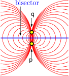
(A)	(B)

Figure 2.1: (A) The unbounded bisector induced by $\mathsf{p}$ and $\mathsf{q}$. (B) The pencil of $\mathsf{p}$ and $\mathsf{q}$.

Definition 2.4.

For a closed set $\mathsf{X}\subseteq{\rm I\!R}^{d}$, and a point $\mathsf{p}\in{\rm I\!R}^{d}$, the projection of $\mathsf{p}$ into $\mathsf{X}$ is the closest point on $\mathsf{X}$ to $\mathsf{p}$. We denote the projected point by $\mathsf{nn}\!\left({\mathsf{p},\mathsf{X}}\right)$.

3 Computing a small Voronoi separator

3.1 Preliminaries, and how to block a sphere

Given a set $\mathsf{P}$ of $n$ points in ${\rm I\!R}^{d}$, we show how to compute a balanced Voronoi separator for $\mathsf{P}$ of size $O\!\left({n^{1-1/d}}\right)$.

Definition 3.1.

A set $\mathsf{Y}\subseteq\mathsf{X}\subseteq{\rm I\!R}^{d}$ is $\ell$-dense in $\mathsf{X}$, if for any point $\mathsf{p}\in\mathsf{X}$, there exists a point $\mathsf{s}\in\mathsf{Y}$, such that $\left\|{\mathsf{p}}-{\mathsf{s}}\right\|\leq\ell$.

Lemma 3.2.

Consider an arbitrary sphere $\mathbb{S}$, and a point $\mathsf{p}\in{\rm I\!R}^{d}\setminus\mathbb{S}$. Then one can compute, in constant time, a set of points $\mathsf{Q}\subseteq\mathbb{S}$, such that the Voronoi cell $\mathcal{C}_{\mathsf{Q}\cup\left\{{\mathsf{p}}\right\}}\!\left({\mathsf{p}}\right)$ does not intersect $\mathbb{S}$, and $\left|{\mathsf{Q}}\right|=O(1)$. We denote the set $\mathsf{Q}$ by $\mathrm{blocker{}Set}\!\left({\mathsf{p},\mathbb{S}}\right)$.

Proof.

If $\mathsf{p}$ is outside the sphere $\mathbb{S}$, then $\mathsf{Q}=\left\{{\mathsf{nn}\!\left({\mathsf{p},\mathbb{S}}\right)}\right\}$ provides the desired separation.

If $\mathsf{p}$ is inside $\mathbb{S}$, then consider the unit sphere centered at $\mathsf{p}$, cover it with the minimum number of spherical caps having diameter $\leq\pi/3$, and let $\mathcal{C}$ be the resulting set of caps. Every such cap of directions defines a natural cone centered at $\mathsf{p}$. Formally, for such a cap $C$, consider the set $\mathrm{cone}\!\left({\mathsf{p},C}\right)=\left\{{\mathsf{p}+t\mathsf{s}\,\left|\,{\mathsf{s}\in C,t\geq 0}\rule[-5.69046pt]{0.0pt}{11.38092pt}\right.}\right\}$. Compute the closest point of $\mathbb{S}$ inside this cone, and add the point to $\mathsf{Q}$. Repeat this process for all the caps of $\mathcal{C}$.

We claim that $\mathsf{Q}$ is the desired blocker. To this end, consider any cap $C\in\mathcal{C}$, and observe that $\mathrm{cone}\!\left({\mathsf{p},C}\right)$ contains $\mathsf{s}\in\mathsf{Q}$, and this is the closest point on $\mathbb{S}\cap\mathrm{cone}\!\left({\mathsf{p},C}\right)$ to $\mathsf{p}$. In particular, since the cone angle is $\leq\pi/3$, it is straightforward to verify that the bisector of $\mathsf{p}$ and $\mathsf{s}$ separates $\mathbb{S}\cap\mathrm{cone}\!\left({\mathsf{p},C}\right)$ from $\mathsf{p}$, implying that $\mathcal{C}_{\mathsf{Q}\cup\left\{{\mathsf{p}}\right\}}\!\left({\mathsf{p}}\right)$ can not intersect the portion of $\mathbb{S}$ inside $\mathrm{cone}\!\left({\mathsf{p},C}\right)$, see figure above for an example.

3.2 The Algorithm

The input is a set $\mathsf{P}$ of $n$ points in ${\rm I\!R}^{d}$. The algorithms works as follows:

1. Let $c_{d}=c^{d}_{\mathrm{dbl}}+1$, see Definition 2.3. Let $\mathrm{ball}\!\left({\psi,{r}}\right)$ be the smallest (closed) ball that contains $n/c_{d}$ points of $\mathsf{P}$ where $\psi\in{\rm I\!R}^{d}$.

2. Pick a number ${r}^{\prime}$ uniformly at random from the range $\left[{{r},2{r}}\right]$.

3. Let $b^{\prime}=\mathrm{ball}\!\left({\psi,{r}^{\prime}}\right)$.

4. Let $\mathsf{P}_{1}=\mathsf{P}\cap b^{\prime}$ and $\mathsf{P}_{2}=\mathsf{P}\setminus b^{\prime}$.

5. Let $\ell={r}^{\prime}/n^{1/d}$. Compute an $\ell$-dense set $\mathcal{Z}$, of size $O\!\left({\!\left({{r}^{\prime}/\ell}\right)^{d-1}}\right)=O\!\left({n^{1-1/d}}\right)$, on the sphere $\mathbb{S}=\partial b^{\prime}$ using the algorithm of Lemma 3.3 described below.

6. If a point $\mathsf{p}\in\mathsf{P}$ is in distance smaller than $\ell$ from $\mathbb{S}$, we insert $\mathrm{blocker{}Set}\!\left({\mathsf{p},\mathbb{S}}\right)$ into the separating set $\mathcal{Z}$, see Lemma 3.2.

Figure 3.1: A slightly inaccurate depiction of how the algorithm works.

We claim that the resulting set $\mathcal{Z}$ is the desired separator.

Efficient implementation.

One can find a $2$-approximation (in the radius) to the smallest ball containing $n/c_{d}$ points in linear time, see [Har11a]. This would slightly deteriorate the constants used above, but we ignore this minor technicality for the sake of simplicity of exposition. If the resulting separator is too large (i.e., larger than $\Omega\!\left({n^{1-1/d}}\right)$ see below for details), we rerun the algorithm.

3.2.1 Computing a dense set

The following is well known, and we include it only for the sake of completeness.

Lemma 3.3.

Given a sphere $\mathbb{S}$ of radius ${r}^{\prime}$ in ${\rm I\!R}^{d}$, and given a number $\ell>0$, one can compute a $\ell$-dense set $\mathsf{X}$ on $\mathbb{S}$ of size $O\!\left({\!\left({{r}^{\prime}/\ell}\right)^{d-1}}\right)$. This set can be computed in $O\!\left({\left|{\mathsf{X}}\right|}\right)$ time.

Proof.

Consider the grid $\mathsf{G}$ of sidelength $\ell/\sqrt{d}$, and let $\mathsf{X}$ be the set of intersection points of the lines of $\mathsf{G}$ with $\mathbb{S}$. Observe that every $(d-1)$-face of the bounding cube of $\mathbb{S}$ intersects $O\!\left({\!\left({{r}^{\prime}/\ell}\right)^{d-1}}\right)$ lines of the grid, and since there $2d$ such faces, the claim on the size of $\mathsf{X}$ follows.

As for the density property, observe that for any point $\mathsf{p}\in\mathbb{S}$, let $C$ be the grid cell of $\mathsf{G}$ that contains it. Observe, that $\mathrm{ball}\!\left({\mathsf{p},\ell}\right)$ contains $C$ completely, one of the vertices of $C$ must be inside the sphere, and at least one of them must be outside the sphere. Since the edges of the boundary of $C$ are connected, it follows that one of the points of $\mathsf{X}$ is on the boundary of $C$, which in turn implies that there is a point of $\mathsf{X}$ contained in $\mathrm{ball}\!\left({\mathsf{p},\ell}\right)$, implying the desired property.

3.3 Correctness

Lemma 3.4.

We have $\left|{\mathsf{P}_{1}}\right|\geq n/c_{d}$ and $\left|{\mathsf{P}_{2}}\right|\geq n/c_{d}$.

Proof.

By Definition 2.3, the ball $b^{\prime}=\mathrm{ball}\!\left({\psi,{r}^{\prime}}\right)$ can be covered by $c^{d}_{\mathrm{dbl}}$ balls of radius ${r}$, each one of them contains at most $n/c_{d}$ points, as $\mathrm{ball}\!\left({\psi,{r}}\right)$ is the smallest ball containing $n/c_{d}$ points of $\mathsf{P}$.

As such $b^{\prime}$ contains at most $c^{d}_{\mathrm{dbl}}n/c_{d}$ points of $\mathsf{P}$. In particular, as $c_{d}=c^{d}_{\mathrm{dbl}}+1$, we have that $b^{\prime}$ has at least $n/c_{d}$ points of $\mathsf{P}$, inside it, and at least $n(1-c^{d}_{\mathrm{dbl}}/c_{d})=n/c_{d}$ points outside it.

Lemma 3.5.

The sets $\mathsf{P}_{1}$ and $\mathsf{P}_{2}$ are Voronoi separated in $\mathcal{V}\!\left({\mathsf{P}\cup\mathcal{Z}}\right)$.

Proof.

We claim that all the points on $\mathbb{S}$ are dominated by $\mathcal{Z}$. Formally, for any $\mathsf{s}\in\mathbb{S}$, we have that $\mathsf{d}\!\left({\mathsf{s},\mathcal{Z}}\right)\leq\mathsf{d}\!\left({\mathsf{p},\mathsf{P}}\right)$, which clearly implies the claim.

So, let $\mathsf{q}$ be the nearest neighbor to $\mathsf{s}$ in $\mathsf{P}$. If $\left\|{\mathsf{s}}-{\mathsf{q}}\right\|\geq\ell$ then since $\mathcal{Z}$ is $\ell$-dense in $\mathbb{S}$, it follows that there exists $\mathsf{t}\in\mathcal{Z}$ such that $\mathsf{d}\!\left({\mathsf{s},\mathcal{Z}}\right)\leq\left\|{\mathsf{s}}-{\mathsf{t}}\right\|\leq\ell\leq\left\|{\mathsf{s}}-{\mathsf{q}}\right\|=\mathsf{d}\!\left({\mathsf{s},\mathsf{P}}\right)$, as desired.

If $\left\|{\mathsf{s}}-{\mathsf{q}}\right\|<\ell$ then the addition of $\mathrm{blocker{}Set}\!\left({\mathsf{q},\mathbb{S}}\right)$ to $\mathcal{Z}$, during the construction, guarantees that the nearest point in $\mathcal{Z}$ to $\mathsf{s}$, is closer to $\mathsf{s}$ than $\mathsf{q}$ is, see Lemma 3.2.

Lemma 3.6.

Let $Y=\left|{\mathcal{Z}}\right|$. We have that $\mathop{\mathbf{E}}\!\left[{Y}\right]\leq c_{\mathrm{sep}}n^{1-1/d}$, where $c_{\mathrm{sep}}$ is some constant.

Proof.

Let $Z$ be the number of points of $\mathsf{P}$, whose projections were added to $\mathcal{Z}$. We claim that $\mathop{\mathbf{E}}\!\left[{Z}\right]=O\!\left({n^{1-1/d}}\right)$. To this end, for a point $\mathsf{p}\in\mathsf{P}$, let $X_{\mathsf{p}}$ be the indicator variable that is one if and only if $\mathsf{p}$ is in distance at most $\ell$ from $\mathbb{S}$. The algorithm picked the radius ${r}^{\prime}$ uniformly at random in the interval $[{r},2{r}]$. Furthermore, $X_{\mathsf{p}}=1$ if and only if $\left\|{\mathsf{p}}-{\psi}\right\|-\ell\leq{r}^{\prime}\leq\left\|{\mathsf{p}}-{\psi}\right\|+\ell$. This happens only if ${r}^{\prime}$ falls into an interval $I_{\mathsf{p}}$ that is of length at most $2\ell$ centered at $\left\|{\mathsf{p}}-{\psi}\right\|$. As such, we have

$$\mathop{\mathbf{Pr}}\!\left[{\rule[-5.69046pt]{0.0pt}{11.38092pt}X_{\mathsf{p}}=1}\right]=\frac{\mathrm{len}\!\left({\rule[0.0pt]{0.0pt}{11.09654pt}I_{\mathsf{p}}\cap[r,2r]}\right)}{\mathrm{len}\!\left({\rule[0.0pt]{0.0pt}{11.09654pt}[r,2r]}\right)}\leq\frac{2\ell}{{r}}=\frac{2\!\left({{r}^{\prime}/n^{1/d}}\right)}{{r}}\leq\frac{4}{n^{1/d}}.$$

Now, by linearity of expectation, we have that $\mathop{\mathbf{E}}\!\left[{Z}\right]=\sum_{\mathsf{p}\in\mathsf{P}}\mathop{\mathbf{E}}\!\left[{cX_{\mathsf{p}}}\right]\leq O(n^{1-1/d})$, where $c$ is the constant of Lemma 3.2. This implies the claim, as $Y=Z+O\!\left({n^{1-1/d}}\right)$.

3.4 The result

Theorem 3.7.

Let $\mathsf{P}$ be a set of $n$ points in ${\rm I\!R}^{d}$. One can compute, in expected linear time, a sphere $\mathbb{S}$, and a set $\mathcal{Z}\subseteq\mathbb{S}$, such that

1. $\left|{\mathcal{Z}}\right|=O\!\left({n^{1-1/d}}\right)$,

2. $\mathbb{S}$ contains $\geq cn$ points of $\mathsf{P}$ inside it,

3. there are $\geq cn$ points of $\mathsf{P}$ outside $\mathbb{S}$, and

4. $\mathcal{Z}$ is a Voronoi separator of the points of $\mathsf{P}$ inside $\mathbb{S}$ from the points of $\mathsf{P}$ outside $\mathbb{S}$.

Here $c>0$ is a constant that depends only on the dimension $d$.

Proof.

Clearly, each round of the algorithm takes $O(n)$ time. By Markov’s inequality the resulting separator set $\mathcal{Z}$ is of size at most $2c_{\mathrm{sep}}n^{1-1/d}$, with probability at least $1/2$, see Lemma 3.6. As such, if the separator is larger than this threshold, then we rerun the algorithm. Clearly, in expectation, after a constant number of iterations the algorithm would succeed, and terminates. (It is not hard to derandomize this algorithm and get a linear running time.)

4 Exact algorithm for computing the optimal separation for a given partition

Given a set $\mathsf{P}$ of $n$ points in ${\rm I\!R}^{d}$, and a partition $\left({\mathsf{P}_{1},\mathsf{P}_{2}}\right)$ of $\mathsf{P}$, we are interested in computing the smallest Voronoi separating set realizing this partition.

4.1 Preliminaries and problem statement

Definition 4.1.

For a set $\mathsf{P}\in{\rm I\!R}^{d}$ and a pair of disjoint subsets $(\mathsf{P}_{1},\mathsf{P}_{2})$, the set of bad pairs is $\mathcal{BP}\!\left({\mathsf{P},\mathsf{P}_{1},\mathsf{P}_{2}}\right)=\left\{{(\mathsf{p}_{1},\mathsf{p}_{2})\in\mathsf{P}_{1}\times\mathsf{P}_{2}\,\left|\,{\,\mathcal{C}_{\mathsf{P}}\!\left({\mathsf{p}_{1}}\right)\cap\mathcal{C}_{\mathsf{P}}\!\left({\mathsf{p}_{2}}\right)\neq\emptyset}\rule[-5.69046pt]{0.0pt}{11.38092pt}\right.}\right\}.$

For a Voronoi diagram $\mathcal{V}\!\left({\mathsf{P}}\right)$, we can assume that all its faces (of various dimensions) are all triangulated (say, using bottom-vertex triangulation). This does not change the complexity of the Voronoi diagram. For $k=0,1,\ldots,d$, such a $k$ dimensional Voronoi simplex is a $k$-feature. Such a $k$-feature $\mathsf{f}$, is induced by $d-k+1$ sites, denoted by $\mathrm{sites}\!\left({\mathsf{f}}\right)$; that is, any point $\mathsf{p}\in\mathsf{f}$ is in equal distance to all the points of $\mathrm{sites}\!\left({\mathsf{f}}\right)$ and these are the nearest neighbor of $\mathsf{p}$ in $\mathsf{P}$. Thus, a vertex $v$ of the Voronoi diagram is a $0$-feature, and $\left|{\mathrm{sites}\!\left({v}\right)}\right|=d+1$ (assuming general position, which we do). The span of a feature $\mathsf{f}$, is the set of points in ${\rm I\!R}^{d}$ that are equidistant to every site in $\mathrm{sites}\!\left({\mathsf{f}}\right)$; it is denoted by $\mathrm{span}\!\left({\mathsf{f}}\right)$ and is the $k$ flat that contains $\mathsf{f}$. A $k$-halfflat is the intersection of a halfspace with a $k$-flat.

Consider any $k$-feature $\mathsf{f}$. The complement set $\mathrm{span}\!\left({\mathsf{f}}\right)\setminus\mathsf{f}$ can be covered by $k+1$ $k$-halfflats of $\mathrm{span}\!\left({\mathsf{f}}\right)$. Specifically, each of these halfflats is an open $k$-halfflat of $\mathrm{span}\!\left({\mathsf{f}}\right)$, whose boundary contains a $(k-1)$-dimensional face of the boundary of $\mathsf{f}$. This set of halfflats of $\mathsf{f}$, is the shell of $\mathsf{f}$, and is denoted by $\mathrm{shell}\!\left({\mathsf{f}}\right)$, see Figure 4.1.

Once the Voronoi diagram is computed, it is easy to extract the “bad features”. Specifically, the set of bad features is

$$\mathcal{F}_{\mathrm{bad}}\!\left({\mathsf{P},\mathsf{P}_{1},\mathsf{P}_{2}}\right)=\left\{{\mathsf{f}\in\mathrm{features}\!\left({\mathcal{V}\!\left({\mathsf{P}}\right)}\right)\,\left|\,{\mathrm{sites}\!\left({\mathsf{f}}\right)\cap\mathsf{P}_{1}\neq\emptyset\text{\; and\; }\mathrm{sites}\!\left({\mathsf{f}}\right)\cap\mathsf{P}_{2}\neq\emptyset}\rule[-5.69046pt]{0.0pt}{11.38092pt}\right.}\right\}.$$

Clearly, given a Voronoi diagram the set of bad features can be computed in linear time in the size of the diagram.

Given a $k$-feature $\mathsf{f}$, it is the convex-hull of $k+1$ points; that is, $\mathsf{f}=\mathcal{CH}\!\left({\mathsf{X}}\right)$, where $\mathsf{X}=\left\{{\mathsf{q}_{1},\ldots,\mathsf{q}_{k+1}}\right\}$. We are interested in finding the closest point in a feature to an arbitrary point $\mathsf{p}$. This is a constant size problem for a fixed $d$, and can be solved in constant time. We denote this closest point by $\mathsf{nn}\!\left({\mathsf{p},\mathsf{f}}\right)=\arg\min_{\mathsf{q}\in\mathsf{f}}\mathsf{d}\!\left({\mathsf{p},\mathsf{q}}\right)$. For the feature $\mathsf{f}$, and any point $\mathsf{p}$, we denote by $\mathrm{pencil}_{\mathsf{f}}\!\left({\mathsf{p}}\right)$ the ball $\mathrm{ball}\!\left({\mathsf{p},\mathsf{d}\!\left({\mathsf{p},\mathrm{sites}\!\left({\mathsf{f}}\right)}\right)}\right)$ (if it is uniquely defined). Furthermore, for an arbitrary set $S$ of points, $\mathrm{pencil}_{\mathsf{f}}\!\left({S}\right)$ denote $\left\{{\mathrm{ball}\!\left({\mathsf{p},\mathsf{d}\!\left({\mathsf{p},\mathrm{sites}\!\left({\mathsf{f}}\right)}\right)}\right)\,\left|\,{\mathsf{p}\in S}\rule[-5.69046pt]{0.0pt}{11.38092pt}\right.}\right\}$. In particular, for any point $\mathsf{p}\in\mathsf{f}$, consider $\mathrm{ball}\!\left({\mathsf{p},\mathsf{d}\!\left({\mathsf{p},\mathsf{P}}\right)}\right)$ – it contains the points of $\mathrm{sites}\!\left({\mathsf{f}}\right)$ on its boundary. The set of all such balls is the pencil of $\mathsf{f}$, denoted by

$$\mathrm{pencil}\!\left({\mathsf{f}}\right)=\left\{{\mathrm{ball}\!\left({\mathsf{p},\mathsf{d}\!\left({\mathsf{p},\mathrm{sites}\!\left({\mathsf{f}}\right)}\right)}\right)\,\left|\,{\mathsf{p}\in\mathsf{f}}\rule[-5.69046pt]{0.0pt}{11.38092pt}\right.}\right\}.$$ (4.1)

The trail of $\mathsf{f}$ is the union of all these balls; that is, $\mathrm{trail}\!\left({\mathsf{f}}\right)=\bigcup_{\mathsf{p}\in\mathsf{f}}\mathrm{ball}\!\left({\mathsf{p},\mathsf{d}\!\left({\mathsf{p},\mathsf{P}}\right)}\right)$. Finally, let $\mathrm{mb}\!\left({\mathsf{f}}\right)$ denote the smallest ball in the pencil of a feature $\mathsf{f}$. Clearly, the center of $\mathrm{mb}\!\left({\mathsf{f}}\right)$ is the point $\mathsf{nn}\!\left({\mathsf{p},\mathsf{f}}\right)$, where $\mathsf{p}$ is some arbitrary point of $\mathrm{sites}\!\left({\mathsf{f}}\right)$. As such, $\mathrm{mb}\!\left({\mathsf{f}}\right)$ can be computed in constant time.

Lemma 4.2.

Let $\mathsf{p}$ be any point and let $\mathsf{f}$ be any $k$-feature. The point $\mathsf{p}$ induces a halfflat of $\mathrm{span}\!\left({\mathsf{f}}\right)$ denoted by $\mathcal{H}\!\left({\mathsf{p},\mathsf{f}}\right)$, such that $\mathrm{pencil}\!\left({\mathcal{H}\!\left({\mathsf{p},\mathsf{f}}\right)}\right)$ is the set of all balls in $\mathrm{pencil}\!\left({\mathrm{span}\!\left({\mathsf{f}}\right)}\right)$ that contain $\mathsf{p}$.

Proof.

Consider any arbitrary site $\mathsf{s}\in\mathrm{sites}\!\left({\mathsf{f}}\right)$. The set of points whose ball in the pencil contains $\mathsf{p}$, is clearly the set of points in $\mathrm{span}\!\left({\mathsf{f}}\right)$ that are closer to $\mathsf{p}$ than to $\mathsf{s}$. This set of points, is a halfspace of ${\rm I\!R}^{d}$ that is not parallel to the $k$-flat $\mathrm{span}\!\left({\mathsf{f}}\right)$. Thus, $\mathcal{H}\!\left({\mathsf{p},\mathsf{f}}\right)=\left\{{\mathsf{q}\,\left|\,{\left\|{\mathsf{q}}-{\mathsf{p}}\right\|\leq\left\|{\mathsf{q}}-{\mathsf{s}}\right\|}\rule[-5.69046pt]{0.0pt}{11.38092pt}\right.}\right\}\cap\mathrm{span}\!\left({\mathsf{f}}\right)$ is the desired halfflat of $\mathrm{span}\!\left({\mathsf{f}}\right)$ induced by $\mathsf{p}$, whose boundary is given by the set of points equidistant to $\mathrm{sites}\!\left({\mathsf{f}}\right)\cup\left\{{\mathsf{p}}\right\}$.

We are now ready to restate our problem in a more familiar language.

Lemma 4.3 (Restatement of problem).

Given a set $\mathsf{P}$ of $n$ points in ${\rm I\!R}^{d}$, and a pair of disjoint subsets $\left({\mathsf{P}_{1},\mathsf{P}_{2}}\right)$, finding a minimum size Voronoi separator realizing separation of $\left({\mathsf{P}_{1},\mathsf{P}_{2}}\right)$, is equivalent to finding a minimum size hitting set of points $\mathcal{Z}$, such that $\mathcal{Z}$ stabs (the interior) of all the balls in the set

$$\mathcal{B}=\mathcal{B}\!\left({\mathsf{P},\mathsf{P}_{1},\mathsf{P}_{2}}\right)=\bigcup_{\mathsf{f}\in\mathcal{F}_{\mathrm{bad}}\!\left({\mathsf{P},\mathsf{P}_{1},\mathsf{P}_{2}}\right)}\mathrm{pencil}\!\left({\mathsf{f}}\right).$$ (4.2)

Proof.

Indeed, a Voronoi separating set $\mathcal{Z}$, must stab all the balls of $\mathcal{B}$, otherwise, there would be Voronoi feature of $\mathcal{V}\!\left({\mathsf{P}\cup\mathcal{Z}}\right)$ that has a generating site in both, $\mathsf{P}_{1}$ and $\mathsf{P}_{2}$.

As for the other direction, consider a set $\mathsf{X}$ that stabs all the balls of $\mathcal{B}$, and observe that if $\mathsf{P}_{1}$ and $\mathsf{P}_{2}$ are not Voronoi separated in $\mathcal{V}\!\left({\mathsf{P}\cup\mathsf{X}}\right)$, then there exists a ball $b$, that has no point of $\mathsf{P}\cup\mathsf{X}$ in its interior, and points from both $\mathsf{P}_{1}$ and $\mathsf{P}_{2}$ on its boundary. But then, this ball must be in the pencil of the Voronoi feature induced by $\mathsf{P}\cap b$. A contradiction to $\mathsf{X}$ stabbing all the balls of $\mathcal{B}$.

4.2 Exact algorithm in ${\rm I\!R}^{d}$

Given a set $\mathsf{P}$ of $n$ points in ${\rm I\!R}^{d}$, a pair of disjoint subsets $(\mathsf{P}_{1},\mathsf{P}_{2})$ of $\mathsf{P}$ and an upper bound $\mathsf{b}$ on the number of guards, we show how one can compute the minimum size Voronoi separator realizing their separation in $n^{O(\mathsf{b})}$ time. Our approach is to construct a small number of polynomial inequalities that are necessary and sufficient conditions for separation, and then use cylindrical algebraic decomposition to find a feasible solution.

Observation 4.4.

For a set of guards $\mathcal{Z}$, a feature $\mathsf{f}$ is completely removed from $\mathcal{V}\!\left({\mathsf{P}\cup\mathcal{Z}}\right)$, if and only if the induced halfflats of the guards, on $\mathrm{span}\!\left({\mathsf{f}}\right)$, cover $\mathsf{f}$. This follows directly from Lemma 4.3 and Lemma 4.2.

Observation 4.5.

Given a set $\mathcal{H}$ of at least $k+1$ halfflats in a $k$-flat, if $\mathcal{H}$ covers the $k$-flat, then there exists a subset of $(k+1)$-halfflats of $\mathcal{H}$, that covers the $k$-flat. This is a direct consequence of Helly’s theorem.

Low dimensional example.

To get a better understanding of the problem at hand, the reader may imagine the subproblem of removing a bad $2$-feature $\mathsf{f}$ (i.e. $\mathsf{f}$ is a triangle) from the Voronoi diagram. We know that a set $\mathcal{Z}$ of $n$ guards removes $\mathsf{f}$ from the Voronoi diagram, if and only if the $n$ $2$-halfflats induced by $\mathcal{Z}$ cover the triangle $\mathsf{f}$. If we add the feature-induced halfflats induced by $\mathsf{f}$ to the above set of halfflats, then the problem of covering the triangle $\mathsf{f}$, reduces to the problem of covering the entire plane with this new set $S$ of $n+3$ halfflats. Then from Observation 4.5, we have that $\mathsf{f}$ is removed from the Voronoi diagram if and only if there are three halfplanes of $S$, that covers the entire plane (there are $O(n^{3})$ such triplets). Lemma 4.9 below show how to convert the condition that any three $2$-halfflats cover the plane, into a polynomial inequality of degree four in the coordinates of the guards.

4.2.1 Constructing the Conditions

Lemma 4.6.

Let $\mathsf{f}$ be a $k$-feature, and $\mathcal{H}$ be a set of $k$-halfflats on $\mathrm{span}\!\left({\mathsf{f}}\right)$. Then, $\mathcal{H}$ covers $\mathsf{f}$ $\iff$ there exists a subset $\mathcal{G}\subseteq\mathcal{H}^{\prime}=\mathcal{H}\cup\mathrm{shell}\!\left({\mathsf{f}}\right)$ of size $k+1$ that covers $\mathrm{span}\!\left({\mathsf{f}}\right)$.

Proof.

If $\mathcal{H}$ covers $\mathsf{f}$, then $\mathcal{H}^{\prime}=\mathcal{H}\cup\mathrm{shell}\!\left({\mathsf{f}}\right)$ covers $\mathrm{span}\!\left({\mathsf{f}}\right)$, as $\mathrm{shell}\!\left({\mathsf{f}}\right)$ covers $\mathrm{span}\!\left({\mathsf{f}}\right)\setminus\mathsf{f}$. Then, by Helly’s theorem (see Observation 4.5), we have that some subset of $\mathcal{H}^{\prime}$ of size $k+1$ covers $\mathrm{span}\!\left({\mathsf{f}}\right)$.

For the other direction, we have that some subset of $\mathcal{H}^{\prime}$ covers $\mathrm{span}\!\left({\mathsf{f}}\right)$ (of size $k+1$). Since $\mathrm{shell}\!\left({\mathsf{f}}\right)$ does not cover any point in $\mathsf{f}$, we have that $\mathcal{H}=\mathcal{H}^{\prime}\setminus\mathrm{shell}\!\left({\mathsf{f}}\right)$ must cover $\mathsf{f}$ completely.

Observation 4.7.

Consider a set $\mathcal{H}$ of $k+1$ $k$-halfflats all contained in some $k$-flat $\mathsf{F}$. We are interested in checking that $\mathcal{H}$ covers $\mathsf{F}$. Fortunately, this can be done by computing the $k+1$ vertices induced by $\mathcal{H}$ on $\mathsf{F}$, and verifying that each one of them is covered by the other halfflat of $\mathcal{H}$. Formally, $\mathcal{H}$ covers $\mathsf{F}$ $\iff$ for every halfflat $h\in\mathcal{H}$, we have that ${\cap_{i\in\mathcal{H}\setminus\{h\}}\partial i}\,\in\,h$.

For a set $\mathsf{P}$ of $d+1$ points in ${\rm I\!R}^{d}$ in general position, let $\mathrm{ball}_{\mathrm{in}}\!\left({\mathsf{P}}\right)$ be the unique ball having all the points of $\mathsf{P}$ on its boundary.

Lemma 4.8.

Consider a $k$-feature $\mathsf{f}$, let $\mathcal{H}$ be a set of halfflats on $\mathrm{span}\!\left({\mathsf{f}}\right)$, and let $\mathcal{Z}$ be the set of guards inducing the halfflats of $\mathcal{H}$. Assume that $\left|{\mathrm{sites}\!\left({\mathsf{f}}\right)}\right|+\left|{\mathcal{Z}}\right|=d+2$. Let $h\in\mathcal{H}$ be a $k$-halfflat induced by a guard $\mathsf{g}$, and let $\mathsf{p}=\bigcap_{i\in\mathcal{H}\setminus\left\{{h}\right\}}\partial i$. Then $\mathsf{p}\in h$ $\iff$ $\mathsf{g}\in\mathrm{ball}_{\mathrm{in}}\!\left({\rule[-5.69046pt]{0.0pt}{11.38092pt}\mathrm{sites}\!\left({\mathsf{f}}\right)\cup\left({\rule[0.0pt]{0.0pt}{10.95415pt}\mathcal{Z}\setminus\left\{{\mathsf{g}}\right\}}\right)}\right)$.

Proof.

The boundary of the induced halfflat of a guard $\mathsf{g}$, is the set of points equidistant to the points of $\mathrm{sites}\!\left({\mathsf{f}}\right)\cup\mathsf{g}$, see Lemma 4.2; equivalently, this is the set containing every point $\mathsf{p}$, such that $\mathrm{pencil}_{\mathsf{f}}\!\left({\mathsf{p}}\right)$ contains $\mathsf{g}$ on its boundary. Furthermore, for any $\mathsf{q}$ inside this induced halfflat, $\mathsf{g}\in\mathrm{pencil}_{\mathsf{f}}\!\left({\mathsf{q}}\right)$. Thus $\mathsf{g}\in\mathrm{pencil}_{\mathsf{f}}\!\left({\mathsf{p}}\right)$ $\iff$ the point $\mathsf{p}\in h$. Also, $\mathsf{p}$ is the point in equal distance to all the points of $\mathrm{sites}\!\left({\mathsf{f}}\right)\cup\mathcal{Z}\setminus\left\{{\mathsf{g}}\right\}$.

A set $\mathcal{Z}$ of $m$ guards in ${\rm I\!R}^{d}$ can be interpreted as a vector in ${\rm I\!R}^{dm}$ encoding the locations of the guards. One can then reduce the requirement that $\mathcal{Z}$ provides the desired separation into a logical formula over the coordinates of this vector.

Lemma 4.9.

Let $\mathsf{f}$ be a bad $k$-feature of $\mathcal{F}_{\mathrm{bad}}\!\left({\mathsf{P},\mathsf{P}_{1},\mathsf{P}_{2}}\right)$, and let $m$ be a parameter. One can compute a boolean sentence $\mathcal{A}_{\mathsf{f}}\!\left({\mathcal{Z}}\right)$ consisting of $m^{O\left({k}\right)}$ polynomial inequalities (of degree $\leq d+2$), over $dm$ variables, such that $\mathcal{A}_{\mathsf{f}}\!\left({\mathcal{Z}}\right)$ is true $\iff$ the set of $m$ guards $\mathcal{Z}$ (induced by the solution of this formula) destroys $\mathsf{f}$ completely when inserted. Formally, for every $\mathsf{f}^{\prime}\in\mathcal{F}_{\mathrm{bad}}\!\left({\mathsf{P}\cup\mathcal{Z},\mathsf{P}_{1},\mathsf{P}_{2}}\right)$, we have $\mathsf{f}\cap\mathsf{f}^{\prime}=\emptyset$.

Proof.

Let $\mathcal{H}=\left\{{\mathcal{H}\!\left({\mathsf{p},\mathsf{f}}\right)\,\left|\,{\mathsf{p}\in\mathcal{Z}}\rule[-5.69046pt]{0.0pt}{11.38092pt}\right.}\right\}$ be the set of halfflats on $\mathrm{span}\!\left({\mathsf{f}}\right)$ induced by the guards in $\mathcal{Z}$. By Observation 4.4, if $\mathcal{H}$ covers $\mathsf{f}$, then $\mathcal{Z}$ removes $\mathsf{f}$ from the Voronoi diagram (see also Lemma 4.3). To this end, let $\mathcal{H}^{\prime}=\mathcal{H}\cup\mathrm{shell}\!\left({\mathsf{f}}\right)$. Further, let $\mathcal{Z}_{\mathsf{f}}$ be a set of $k+1$ points that exactly induce the halfflats of $\mathrm{shell}\!\left({\mathsf{f}}\right)$ and let $\mathcal{Z}^{\prime}=\mathcal{Z}\cup\mathcal{Z}_{\mathsf{f}}$. From Lemma 4.6, we know that $\mathcal{H}$ covers $\mathsf{f}$ $\iff$ some size $k+1$ subset of $\mathcal{H}^{\prime}$ covers the $k$-flat $\mathrm{span}\!\left({\mathsf{f}}\right)$. Then by Observation 4.7, $\mathcal{H}$ covers $\mathsf{f}$ $\iff$ there exists some size $k+1$ subset $\mathcal{H}_{1}$ of $\mathcal{H}^{\prime}$, such that for every $h\in\mathcal{H}_{1}$, we have $\bigcap_{i\in\mathcal{H}_{1}\setminus h}\partial i\in h$.

Since $\mathcal{Z}^{\prime}$ exactly induces the halfflats of $\mathcal{H}^{\prime}$, Lemma 4.8 implies that $\mathsf{f}$ is completely removed from $\mathcal{V}\!\left({\mathsf{P}\cup\mathcal{Z}}\right)$ $\iff$ there exists some size $k+1$ subset $\mathcal{Z}_{1}$ of $\mathcal{Z}^{\prime}$, such that for every $\mathsf{g}\in\mathcal{Z}_{1}$, $\mathsf{g}$ lies inside the ball containing the points of $\mathrm{sites}\!\left({\mathsf{f}}\right)\cup\!\left({\mathcal{Z}_{1}\setminus\mathsf{g}}\right)$ on its boundary. More formally, we define,

$$\mathcal{A}_{\mathsf{f}}\!\left({\mathcal{Z}}\right)\qquad\equiv\qquad\bigvee_{\mathcal{Z}_{1}\subseteq\mathcal{Z}^{\prime},\left|{\mathcal{Z}_{1}}\right|=k+1}\!\left({\bigwedge_{\mathsf{g}\in\mathcal{Z}_{1}}\!\!\left[{\mathcal{ID}\!\left({\rule[-5.69046pt]{0.0pt}{11.38092pt}\mathrm{sites}\!\left({\mathsf{f}}\right)\cup\!\left({\mathcal{Z}_{1}\setminus\mathsf{g}}\right),\mathsf{g}}\right)\leq 0}\rule[-5.69046pt]{0.0pt}{11.38092pt}\right]}\right),$$

where $\mathcal{ID}\!\left({S,\mathsf{p}}\right)$ represents the standard in-circle determinant whose sign determines the inclusion of $\mathsf{p}$ in the ball fixed by the points of $S$. This determinant affords us a polynomial of degree at most $d+2$ involving only the variables of $\mathcal{Z}$, as the points of $\mathcal{Z}_{\mathsf{f}}$ are merely constants. Clearly, $\mathcal{A}_{\mathsf{f}}\!\left({\mathcal{Z}}\right)$ contains at most $\left|{\mathcal{Z}}\right|^{O\left({k}\right)}$ polynomial inequalities, and the claim follows.

4.2.2 The Result

Theorem 4.10.

Let $\mathsf{P}$ be a set of $n$ points in ${\rm I\!R}^{d}$. Let $(\mathsf{P}_{1},\mathsf{P}_{2})$ be some disjoint partition of $\mathsf{P}$ and $\mathsf{b}$ be a parameter, such that there exists a Voronoi separator for $(\mathsf{P}_{1},\mathsf{P}_{2})$ of at most $\mathsf{b}$ points. The minimal size Voronoi separator can be computed in $n^{O\left({\mathsf{b}}\right)}$ time, if such a separator exists of size at most $\mathsf{b}$ (note, that the constant in the $O$ notations depends on $d$).

Proof.

Let $\mathrm{g}$ be a parameter to be fixed shortly. Let $\mathcal{Z}$ be a set of $\mathrm{g}$ guards in ${\rm I\!R}^{d}$. By Lemma 4.9, the condition $\mathcal{A}\!\left({\mathcal{Z}}\right)$ that every bad feature is removed from the Voronoi diagram of $\mathsf{P}\cup\mathcal{Z}$, can be written as

$$\mathcal{A}\!\left({\mathcal{Z}}\right)=\bigwedge_{\mathsf{f}\in\mathcal{F}_{\mathrm{bad}}\left({\mathsf{P},\mathsf{P}_{1},\mathsf{P}_{2}}\right)}\mathcal{A}_{\mathsf{f}}\!\left({\mathcal{Z}}\right).$$

Namely, $\mathcal{Z}$ is a Voronoi separator for $(\mathsf{P}_{1},\mathsf{P}_{2})$. The formula $\mathcal{A}\!\left({\mathcal{Z}}\right)$ contains $n^{O\left({d}\right)}$ degree-$d+2$ polynomial inequalities comprising of at most $d\mathrm{g}$ variables. By [BPR06, Theorem 13.12], one can compute, in $n^{O\left({\mathrm{g}}\right)}$ time, a solution as well as the sign of each polynomial in $\mathcal{P}$, for every possible sign decomposition that $\mathcal{P}$ can attain. Now for each attainable sign decomposition, we simply check if $\mathcal{A}\!\left({\mathcal{Z}}\right)$ is true. This can be done in $n^{O\left({d}\right)}$ time. The algorithm computes a Voronoi separator for $(\mathsf{P}_{1},\mathsf{P}_{2})$ in $\mathsf{P}$ of size $\mathrm{g}$, in $n^{O\left({\mathrm{g}}\right)}$ time, if such a separator exists.

Now, the algorithms tries $\mathrm{g}=1,\ldots,\mathsf{b}$ and stops as soon as a feasible solution is found.

Remark.

Interestingly, both here and in the rest of the paper, one can specify which pair of points need to be separated from each other (instead of a partition of the input set), and the algorithm works verbatim for this case (of course, in the worst case, one might need to specify $O(n^{2})$ pairs, if one explicitly lists the forbidden pairs).

5 Approximation algorithms

5.1 Constant factor approximation

Given a set $\mathsf{P}$ of $n$ points in ${\rm I\!R}^{d}$, and a partition $(\mathsf{P}_{1},\mathsf{P}_{2})$ of $\mathsf{P}$, we show how one can compute in $n^{O(d)}$ time, a Voronoi separator $\mathcal{Z}$ for $(\mathsf{P}_{1},\mathsf{P}_{2})$, whose size is a constant factor approximation to the size of the minimal Voronoi separator realizing such a partition.

5.1.1 The algorithm GreedySeparator

Since the problem is equivalent to a hitting set problem on balls, see Lemma 4.3, we can apply the “standard” greedy strategy. Specifically, given $\mathsf{P}\subseteq{\rm I\!R}^{d}$, and a pair of disjoint subsets $\left({\mathsf{P}_{1},\mathsf{P}_{2}}\right)$, start with an empty set $\mathsf{X}$ of stabbing points.

Now, at each iteration, compute the Voronoi diagram $\mathcal{V}\!\left({\mathsf{P}\cup\mathsf{X}}\right)$, and compute the set of bad features $\mathcal{F}_{\mathrm{bad}}\!\left({\mathsf{P}\cup\mathsf{X},\mathsf{P}_{1},\mathsf{P}_{2}}\right)$. Compute the minimum ball in $\mathrm{pencil}\!\left({\mathsf{f}}\right)$ (see Eq. (4.1)) for each of the bad features $\mathsf{f}\in\mathcal{F}_{\mathrm{bad}}\!\left({\mathsf{P}\cup\mathsf{X},\mathsf{P}_{1},\mathsf{P}_{2}}\right)$. Let $b=\mathrm{ball}\!\left({\mathsf{p},r}\right)$ be the smallest ball encountered. Let $\mathsf{P}_{b}$ be a constant size set of points, such that any ball that intersects $b$ (and is at least as large), must intersect $\mathsf{P}_{b}$. Such a set can be easily constructed by sprinkling a $r$-dense set in the enlarged ball $\mathrm{ball}\!\left({\mathsf{p},2r}\right)$. Note that $\mathsf{P}_{b}$ must also stab $b$. The resulting set $\mathsf{P}_{b}$ has constant size (for example, by using grid points of the appropriate size). Set $\mathsf{X}\leftarrow\mathsf{X}\cup\mathsf{P}_{b}$, and repeat.

5.1.2 The Result

Theorem 5.1.

Let $\mathsf{P}$ be a set of $n$ points in ${\rm I\!R}^{d}$, and $\left({\mathsf{P}_{1},\mathsf{P}_{2}}\right)$ be a given pair of disjoint subsets of $\mathsf{P}$. One can compute a Voronoi separator $\mathcal{Z}$ that realizes this partition. The algorithm runs in $O(n^{2}\log n)$ time for $d=2$, and in $O\!\left({n^{\left\lceil{d/2}\right\rceil+1}}\right)$ time, for $d>2$. The algorithm provides a constant factor approximation to the smallest Voronoi separator realizing this partition.

Proof.

Observe the optimal solution is finite, as one can place $d+1$ points around each point of $\mathsf{P}_{1}$, close enough, so that they Voronoi separate this point from the rest of $\mathsf{P}$. As such, the optimal solution is of size at most $(d+1)\min\!\left({\left|{\mathsf{P}_{1}}\right|,\left|{\mathsf{P}_{2}}\right|}\right)$.

As for the quality of approximation, this is a standard exchange argument. Indeed, consider the optimal solution, and observe that, at each iteration, the minimum ball found $b$ must contain at least one point of the optimal solution, and the greedy algorithm replaces it in the approximation by the set $\mathsf{P}_{b}$, such that any ball that is stabbed by a point of the optimal solution that is contained in $b$, and is at least as big as $b$ is also stabbed by some points of $\mathsf{P}_{b}$. In particular, if $c$ is the maximum size set $\mathsf{P}_{b}$ constructed by the algorithm (which is a constant), then the quality of approximation of the algorithm is $c$.

The above implies that the algorithms terminates with at most $O(n)$ points added. Since computing the Voronoi diagram takes $O(n\log n)$ time in the plane, this implies that the running of the algorithm in the plane is $O(n^{2}\log n)$. In higher dimensions, computing the Voronoi diagram takes $O\!\left({n^{\left\lceil{d/2}\right\rceil}}\right)$, and overall, the algorithm takes $O\!\left({n^{\left\lceil{d/2}\right\rceil+1}}\right)$ time.

5.2 Polynomial time approximation scheme

Given a set $\mathsf{P}$ of $n$ points in ${\rm I\!R}^{d}$, a parameter ${\varepsilon}>0$, and a pair of disjoint subsets $(\mathsf{P}_{1},\mathsf{P}_{2})$ of $\mathsf{P}$, we show here how to $(1+{\varepsilon})$-approximate, in $n^{O(1/{\varepsilon}^{d})}$ time, a Voronoi separator $\mathcal{Z}$ for $(\mathsf{P}_{1},\mathsf{P}_{2})$.

As implied by Lemma 4.3, this problem boils down to a hitting set problem. That is, the desired partition give rise to a set of balls $\mathcal{B}$, such that our task is to approximate the minimum size hitting set for $\mathcal{B}$. The challenge here is that $\mathcal{B}$ is an infinite set, see Eq. (4.2)${}_{\text{p\ref{equation:hitting:set}}}$.

We need an improved separator theorem, as follows.

Theorem 5.2.

Let $\mathsf{X}$ be a set of points in ${\rm I\!R}^{d}$, and $k>0$ be an integer sufficiently smaller than $\left|{\mathsf{X}}\right|$. One can compute, in $O\!\left({\left|{\mathsf{X}}\right|}\right)$ expected time, a set $\mathcal{Z}$ of $O\!\left({k^{1-1/d}}\right)$ points and a sphere $\mathbb{S}$ containing $\Theta(k)$ points of $\mathsf{X}$ inside it, such that for any set $\mathcal{B}$ of balls stabbed by $\mathsf{X}$, we have that every ball of $\mathcal{B}$ that intersects $\mathbb{S}$ is stabbed by a point of $\mathcal{Z}$.

Due to space limitations, we had delegated the proof of Theorem 5.2 to Appendix A – it is a careful extension of the proof of Theorem 3.7.

5.2.1 Preliminaries

For a set $\mathcal{B}$ of balls in ${\rm I\!R}^{d}$, let $\nu\!\left({\mathcal{B}}\right)$ be the size of its minimal hitting set. Here, our aim is to approximate the value of $\nu\!\left({\mathcal{B}\!\left({\mathsf{P},\mathsf{P}_{1},\mathsf{P}_{2}}\right)}\right)$.

Observation 5.3.

Let $\mathcal{B}$ and $\mathcal{B}^{\prime}$ be sets of balls such that $\mathcal{B}^{\prime}\subseteq\mathcal{B}$. Then $\nu\!\left({\mathcal{B}^{\prime}}\right)\leq\nu\!\left({\mathcal{B}}\right)$.

Observation 5.4.

Let $\mathcal{B}$ and $\mathcal{B}^{\prime}$ be sets of balls such that no ball in $\mathcal{B}$ intersects a ball in $\mathcal{B}^{\prime}$. Then $\nu\!\left({\mathcal{B}\cup\mathcal{B}^{\prime}}\right)=\nu\!\left({\mathcal{B}}\right)+\nu\!\left({\mathcal{B}^{\prime}}\right)$.

5.2.2 The Algorithm ApproximateSeparator

The input is a set $\mathsf{P}$ of $n$ points in ${\rm I\!R}^{d}$, and a desired partition $\left({\mathsf{P}_{1},\mathsf{P}_{2}}\right)$.

1. Using the algorithm GreedySeparator, compute a Voronoi separator $\mathsf{X}$, for $(\mathsf{P}_{1},\mathsf{P}_{2})$ in $\mathsf{P}$, and let $k=O\!\left({1/{\varepsilon}^{d}}\right)$.

2. $i\leftarrow 1$

3. $\mathsf{X}_{1}\leftarrow\mathsf{X}$, $\mathcal{Z}_{1}=\emptyset$

4. While $\mathsf{X}_{i}\neq\emptyset$:

   1. Compute a sphere $\mathbb{S}_{i}$ and a set $\mathcal{Z}^{\mathbb{S}}_{i}$ using Theorem 5.2 for $\mathsf{X}_{i}$ with the parameter $\min\!\left({k,\left|{\mathsf{X}_{i}}\right|}\right)$.

   2. Let $b_{i}$ be the corresponding closed ball of $\mathbb{S}_{i}$.

   3. $\mathsf{Q}_{i}\leftarrow(\mathsf{P}\cap b_{i})\cup\mathcal{Z}_{i}\cup\mathcal{Z}^{\mathbb{S}}_{i}$,  $\mathsf{P}_{i,1}=b_{i}\cap\mathsf{P}_{1}$,  $\mathsf{P}_{i,2}=b_{i}\cap\mathsf{P}_{2}$,  $\Xi_{i}=b_{i}\cap\mathsf{X}_{i}$.

   4. $\mathcal{Z}_{i}^{\prime}\leftarrow$ Compute (exactly) the smallest hitting set for $\mathcal{B}\!\left({\mathsf{Q}_{i},\mathsf{P}_{i,1},\mathsf{P}_{i,2}}\right)$ using Theorem 4.10.

   5. $\mathsf{X}_{i+1}\leftarrow\mathsf{X}_{i}\setminus b_{i}$

   6. $\mathcal{Z}_{i+1}\leftarrow\mathcal{Z}_{i}\cup\mathcal{Z}^{\mathbb{S}}_{i}\cup\mathcal{Z}_{i}^{\prime}$

   7. $i\leftarrow i+1$

5. Output $\mathcal{Z}_{i}$

5.2.3 Correctness

Let $t$ be the number of iterations in the algorithm above. Let $\mathcal{B}=\mathcal{B}\!\left({\mathsf{P},\mathsf{P}_{1},\mathsf{P}_{2}}\right)$ be the set of all balls that need to be hit (see Eq. (4.2)${}_{\text{p\ref{equation:hitting:set}}}$). For $i=1,\ldots,t$, let $\mathcal{B}_{i}=\mathcal{B}\!\left({\mathsf{Q}_{i},\mathsf{P}_{i,1},\mathsf{P}_{i,2}}\right)$.

Lemma 5.5.

The set $\mathcal{Z}_{t}$ is a hitting set for $\mathcal{B}$.

Proof.

Observe that $\Xi_{1},\ldots,\Xi_{t}$ form a partition of $\mathsf{X}$, and consider any ball $b^{\prime}\in\mathcal{B}$. The ball $b^{\prime}$ is stabbed by at least one point of $\mathsf{X}$, and let $j$ be the minimal index such that $\Xi_{j}$ stabs $b^{\prime}$.

If $b^{\prime}$ intersects the sphere $\mathbb{S}_{j}$ then, $\mathcal{Z}^{\mathbb{S}}_{j}\subseteq\mathcal{Z}_{t}$ stabs $b^{\prime}$, by Theorem 5.2. Otherwise, $b^{\prime}$ must be inside $\mathbb{S}_{j}$, as otherwise it cannot be stabbed by the points of $\Xi_{j}\subseteq b_{j}$. But then, $b^{\prime}$ being a “bad” ball, must have a point of $\mathsf{P}_{j,1}$ and a point of $\mathsf{P}_{j,2}$ on its boundary, implying $b^{\prime}\in\mathcal{B}_{j}=\mathcal{B}\!\left({\mathsf{Q}_{j},\mathsf{P}_{j,1},\mathsf{P}_{j,2}}\right)$, and it is thus stabbed by $\mathcal{Z}_{j}^{\prime}\subseteq\mathcal{Z}_{t}$, as testified by Theorem 4.10.

Lemma 5.6.

$\nu\!\left({\bigcup_{i=1}^{t}\mathcal{B}_{i}}\right)=\sum_{i=1}^{t}\nu\!\left({\mathcal{B}_{i}}\right).$

Proof.

Consider any integers $i,j$ such that $1\leq i<j\leq t$. Consider any ball $b\in\mathcal{B}_{i}$. By construction, $\mathcal{Z}_{i}^{\prime}$ stabs $b$. Now $\mathcal{Z}_{i}^{\prime}\subseteq\mathcal{Z}_{j}\subseteq\mathsf{Q}_{j}$, implying that $b$ is stabbed by $\mathsf{Q}_{j}$. Thus, $b$ cannot be in the set $\mathcal{B}_{i}$, and further, $\mathcal{B}_{i}\cap\mathcal{B}_{j}=\emptyset$.

A stronger property holds – there is no point that stabs balls that are in both $\mathcal{B}_{i}$ and $\mathcal{B}_{j}$. Indeed, all the balls of $\mathcal{B}_{i}$ (resp. $\mathcal{B}_{j}$) are contained inside $\mathbb{S}_{i}$ (resp. $\mathbb{S}_{j}$) by Theorem 5.2. As such, such a point $\mathsf{p}$ that stabs balls in both sets, must be in $b_{i}\cap b_{j}$. But $\mathcal{Z}_{i+1}$ stabs all the balls of $\mathcal{B}$ that intersect $b_{i}$. In particular, as $\mathcal{Z}_{i+1}\subseteq\mathsf{Q}_{j}$, it follows that no ball of $\mathcal{B}_{j}$ can intersect $b_{i}$.

Now Observation 5.4 implies the claim.

Lemma 5.7.

Let $m$ be the size of the optimal hitting set. We have $\left|{\mathcal{Z}_{t}}\right|\leq m\!\left({1+O\!\left({1/k^{1/d}}\right)}\right)$.

Proof.

We have $t\leq\left\lceil{\left|{\mathsf{X}}\right|/k}\right\rceil+1=O(m/k)$, as $\mathsf{X}$ is a constant approximation to the optimal hitting set. Then, by Lemma 5.6 and Observation 5.3, we have

$$\left|{\mathcal{Z}_{t}}\right| \leq\sum_{i=1}^{t}\!\left({\left|{\mathcal{Z}_{i}^{\prime}}\right|+\left|{\mathcal{Z}^{\mathbb{S}}_{i}}\right|}\right)\leq\sum_{i=1}^{t}\left|{\mathcal{Z}_{i}^{\prime}}\right|+t\cdot O\!\left({k^{1-1/d}}\right)\leq\sum_{i=1}^{t}\nu\!\left({\mathcal{B}_{i}}\right)+O\!\left({\frac{m}{k^{1/d}}}\right)$$

$$=\nu\!\left({\bigcup_{i=1}^{t}\mathcal{B}_{i}}\right)+O\!\left({\frac{m}{k^{1/d}}}\right)\leq\nu\!\left({\mathcal{B}}\right)+O\!\left({\frac{m}{k^{1/d}}}\right)=m\!\left({1+O\!\left({\frac{1}{k^{1/d}}}\right)}\right).$$

5.2.4 The result

Theorem 5.8.

Given a set $\mathsf{P}$ of $n$ points in ${\rm I\!R}^{d}$, a parameter ${\varepsilon}>0$, and a corresponding partition $(\mathsf{P}_{1},\mathsf{P}_{2})$, one can compute a Voronoi separator for $(\mathsf{P}_{1},\mathsf{P}_{2})$ in $n^{O\left({1/{\varepsilon}^{d}}\right)}$ time, such that its size is a $(1+{\varepsilon})$-approximation to the minimal Voronoi separator realizing the partition $(\mathsf{P}_{1},\mathsf{P}_{2})$.

Proof.

By Lemma 5.5 and Lemma 5.7, setting $k=c/{\varepsilon}^{d}$, where $c$ is a sufficiently large constant implies the desired approximation.

As for the running time, observe that the bottleneck in the running time, is in the invocation of the exact algorithm of Theorem 4.10 in the $i$th iteration, for $i=1,\ldots,t$. However, in the $i$th iteration, a trivial stabbing set is $\Xi_{i}$, which has size $O(k)$. That is, the running time of algorithm of Theorem 4.10 in the $i$th iteration is $n^{O(k)}$, implying the result.

6 PTAS for geometric hitting set via local search

Here, we present a simple local search $(1+{\varepsilon})$-approximation algorithm (PTAS) for hitting set problems of balls (or fat objects) in ${\rm I\!R}^{d}$. The set of balls is either specified explicitly, or as in the case of the Voronoi partition, implicitly.

6.1 The Algorithm LocalHitBalls

6.1.1 Preliminaries

Let $\mathcal{B}$ be a set of balls (possibly infinite) in ${\rm I\!R}^{d}$ that is represented (potentially implicitly) by an input of size $n$, and let $\nu\!\left({\mathcal{B}}\right)$ be the size of its minimal hitting set. We assume that $\mathcal{B}$ satisfies the following properties:

1. Initial solution: One can compute a hitting set $\mathsf{X}_{0}$ of $\mathcal{B}$ in $n^{O\left({1}\right)}$ time, such that the size of $\mathsf{X}_{0}$ is a constant factor approximation to the optimal.

2. Local exchange: Let $\mathsf{X}$ and $\mathsf{Y}$ be point sets, such that

   1. $\mathsf{X}$ is a hitting set of $\mathcal{B}$ (i.e., it is the current solution),

   2. $\left|{\mathsf{X}}\right|\leq n^{O\left({1}\right)}$ (i.e., it is not too large),

   3. $\mathsf{Y}\subseteq\mathsf{X}$ (i.e., $Y$ is the subset to be replaced),

   4. $\left|{\mathsf{Y}}\right|\leq\ell$, where $\ell$ is any integer.

   Then one can compute in $n^{O\left({\ell}\right)}$ time, the smallest set $\mathsf{Y}^{\prime}$, such that $\!\left({\mathsf{X}\setminus\mathsf{Y}}\right)\cup\mathsf{Y}^{\prime}$ is a hitting set of $\mathcal{B}$.

6.1.2 Algorithm

The input is a set $\mathcal{B}$ of balls in ${\rm I\!R}^{d}$ satisfying the properties above. The algorithm works as follows:

1. Compute an initial hitting set $\mathsf{X}_{0}$ of $\mathcal{B}$ (see (P1)), and set $\mathsf{X}\leftarrow\mathsf{X}_{0}$.

2. While there is a beneficial exchange of size $\leq\ell=O\!\left({1/{\varepsilon}^{d}}\right)$ in $\mathsf{X}$, carry it out using (P2).

   Specifically, verify for every subset $\mathsf{Y}\subseteq\mathsf{X}$ of size at most $\ell$, if it can be replaced by a strictly smaller set $\mathsf{Y}^{\prime}$ such that $\!\left({\mathsf{X}\setminus\mathsf{Y}}\right)\cup\mathsf{Y}^{\prime}$ remains a hitting set of $\mathcal{B}$. If so, set $\mathsf{X}\leftarrow\!\left({\mathsf{X}\setminus\mathsf{Y}}\right)\cup\mathsf{Y}^{\prime}$, and repeat.

3. If no such set exists, then return $\mathsf{X}$ as the hitting set.

Details.

For the geometric hitting set problem where $\mathcal{B}$ is a set of $n$ balls in ${\rm I\!R}^{d}$, (P1) follows by a simple greedy algorithm hitting the smallest ball (in the spirit of Theorem 5.1${}_{\text{p\ref{theorem:const:sep}}}$) – see also [Cha03]. As for (P2), one can check for a smaller hitting set of size at most $\ell$ by computing the arrangement $\mathcal{A}\!\left({\mathcal{B}}\right)$, and directly enumerating all possible hitting sets of size at most $\ell$.

The more interesting case is when the set $\mathcal{B}$ is defined implicitly by an instance of the minimal Voronoi separation problem (i.e., we have a set $\mathsf{P}$ of $n$ points in ${\rm I\!R}^{d}$, and a desired Voronoi partition $\!\left({\mathsf{P}_{1},\mathsf{P}_{2}}\right)$ of $\mathsf{P}$). Then (P1) follows from Theorem 5.1. Furthermore, (P2) follows from the algorithm of Theorem 4.10${}_{\text{p\ref{theorem:exact}}}$ through computing the minimal hitting set $\mathsf{Y}^{\prime}$ of $\mathcal{B}\!\left({\mathsf{P}\cup\left({\mathsf{X}\setminus\mathsf{Y}}\right),\mathsf{P}_{1},\mathsf{P}_{2}}\right)$, in $n^{O\left({\ell}\right)}$ time, where $\left|{\mathsf{Y}^{\prime}}\right|\leq\ell$.

ClusterLocalOpt($\mathcal{B}$, $\mathcal{L}$, $\mathcal{O}$): // $\mathcal{B}$: given set of balls need hitting. // $\mathcal{L}\subseteq{\rm I\!R}^{d}$: locally optimal hitting set of $\mathcal{B}$ computed by LocalHitBalls. // $\mathcal{O}\subseteq{\rm I\!R}^{d}$: optimal hitting set. $k:=O\!\left({1/{\varepsilon}^{d}}\right)$,  $\mathsf{L}_{1}:=\mathcal{L}$,  $\mathsf{O}_{1}:=\mathcal{O}$,  $\mathcal{Z}_{1}:=\emptyset$,  $\mathcal{B}_{1}:=\mathcal{B}$,  and $i:=1$. while $\mathsf{L}_{i}\cup\mathcal{Z}_{i}\neq\emptyset$ do Apply Theorem 5.2${}_{\text{p\ref{theorem:ball:separator}}}$ to $\mathsf{L}_{i}\cup\mathcal{Z}_{i}$ with the parameter $\min\!\left({k,\left|{\mathsf{L}_{i}\cup\mathcal{Z}_{i}}\right|}\right)$. $b_{i}$, $T_{i}$: ball and the separator set returned, respectively. $f_{i}:=b_{i}\setminus{\bigcup_{j=1}^{i-1}b_{j}}$ be the region of space newly covered by $b_{i}$. $\mathcal{L}_{i}:=\mathcal{L}\cap f_{i}$ and $\mathcal{O}_{i}=\mathcal{O}\cap f_{i}$. $\mathcal{Z}_{i+1}:=\left({\mathcal{Z}_{i}\setminus b_{i}}\right)\cup T_{i}$. $\mathsf{L}_{i+1}:=\mathsf{L}_{i}\setminus\mathcal{L}_{i}$. $i:=i+1$ $I:=i$.

Figure 6.1: Clustering the local optimal solution.

6.2 Quality of approximation

The bound on the quality of approximation follows by a clustering argument similar to the PTAS algorithm. The clustering is described in Figure 6.1. This breaks up the local optimal solution $\mathcal{L}$ and the optimal solution $\mathcal{O}$ into small sets, and we will use a local exchange argument to bound their corresponding sizes. The following lemma testifies that this clustering algorithm provides a “smooth” way to move from $\mathcal{L}$ to $\mathcal{O}$, through relatively small steps.

Lemma 6.1.

Any ball of $\mathcal{B}$ is stabbed by $\mathsf{X}_{i+1}=\mathsf{L}_{i+1}\cup\mathcal{Z}_{i+1}\cup{\bigcup_{j=1}^{i}\mathcal{O}_{j}}$, for all $i$, where $\mathsf{L}_{i+1}={\bigcup_{j=i+1}^{I}\mathcal{L}_{i}}$.

Proof.

The claim holds clearly for $i=0$, as $\mathsf{L}_{1}=\mathcal{L}$, where $\mathcal{L}$ is the locally optimal solution. Now, for the sake of contradiction, consider the minimum $i$ for which the claim fails, and let $b\in\mathcal{B}$ be the ball that is not being stabbed. We have that $b$ is stabbed by $\mathsf{X}_{i}=\left({\bigcup_{j=i}^{I}\mathcal{L}_{i}}\right)\cup\mathcal{Z}_{i}\cup\left({\bigcup_{j=1}^{i-1}\mathcal{O}_{j}}\right)$ but not by $\mathsf{X}_{i+1}$.

It can not be that $b$ is stabbed by a point of $\bigcup_{j=1}^{i-1}\mathcal{O}_{j}$, as such a point is also present in $\mathsf{X}_{i+1}$. As such, $b$ must be stabbed by one of the points of $\mathsf{L}_{i}\cup\mathcal{Z}_{i}$, and then this stabbing point must be inside $b_{i}$ – indeed, the points removed from $\mathsf{L}_{i}$ and $\mathcal{Z}_{i}$ as we compute $\mathsf{L}_{i+1}$ and $\mathcal{Z}_{i+1}$, respectively, are the ones inside $b_{i}$.

Now, if $b$ intersects $\partial b_{i}$, then $T_{i}\subseteq\mathcal{Z}_{i+1}$ stabs $b$ by Theorem 5.2${}_{\text{p\ref{theorem:ball:separator}}}$, a contradiction.

So it must be that $b\subseteq b_{i}$. But then consider the region $F_{i}=\cup_{j=1}^{i}f_{j}=\cup_{j=1}^{i}b_{j}$. It must be that $b\subseteq F_{i}$. This in turn implies that the point of $\mathcal{O}$ stabbing $b$ is in $\mathcal{O}\cap F_{i}=\cup_{j=1}^{i}\mathcal{O}_{i}\subseteq\mathsf{X}_{i+1}$. A contradiction.

Lemma 6.2.

Consider any ball that $b\in\mathcal{B}$. Let $i$ be the minimum index such that $\mathcal{O}_{i}$ stabs $b$. Then $b$ is stabbed by $\mathcal{L}_{i}\cup T_{i}\cup\left({\mathcal{Z}_{i}\cap b_{i}}\right)$. That is $o_{i}\leq\lambda_{i}+t_{i}+z_{i}$, where $o_{i}=\left|{\mathcal{O}_{i}}\right|$, $t_{i}=\left|{T_{i}}\right|$, and $z_{i}=\left|{\mathcal{Z}_{i}\cap b_{i}}\right|$. Additionally, $o_{i}=O(k)$, for all $i$.

Proof.

If $b$ intersects $\partial b_{i}$, then it is stabbed by $T_{i}$ by Theorem 5.2${}_{\text{p\ref{theorem:ball:separator}}}$. Otherwise, $b\subseteq F_{i}=\cup_{j=1}^{i}f_{j}=\cup_{j=1}^{i}b_{j}$. In particular, this implies that no later point of $\mathcal{O}_{i+1}\cup\ldots\cup\mathcal{O}_{t}$ can stab $b$. That is, only $\mathcal{O}_{i}$ stabs $b$. By Lemma 6.1 both $\mathsf{X}_{i}$ and $\mathsf{X}_{i+1}$ stab $b$, where $\mathsf{X}_{i}=\left({\mathcal{L}\setminus F_{i-1}}\right)\cup\mathcal{Z}_{i}\cup\bigcup_{j=1}^{i-1}\mathcal{O}_{j}$. Namely, $b$ is stabbed by a point of $\left({\mathcal{L}\setminus F_{i-1}}\right)\cup\mathcal{Z}_{i}$ that is contained inside $b_{i}$. Such a point is either in $\mathcal{Z}_{i}\cap b_{i}$, or in $\left({\mathcal{L}\setminus F_{i-1}}\right)\cap b_{i}=\mathcal{L}_{i}$, as claimed.

The second part follows by observing that otherwise $\mathcal{O}_{i}$ can be replaced by $\mathcal{L}_{i}\cup T_{i}\cup\left({\mathcal{Z}_{i}\cap b_{i}}\right)$ in the optimal solution.

The third claim follows by observing that by the algorithm design $\lambda_{i}+z_{i}=O(k)$, and $t_{i}=O\left({k^{1-1/d}}\right)$. As such, $o_{i}\leq\lambda_{i}+t_{i}+z_{i}=O(k)$.

Lemma 6.3.

Consider any ball $b\in\mathcal{B}$ that is stabbed by $\mathcal{L}_{i}$ but it is not stabbed by $\mathcal{L}\setminus\mathcal{L}_{i}$, then $b$ is stabbed by $\mathcal{O}_{i}\cup T_{i}\cup\left({\mathcal{Z}_{i}\cap b_{i}}\right)$. Additionally, using the notations of Lemma 6.2, we have $\lambda_{i}\leq o_{i}+t_{i}+z_{i}$.

Proof.

If $b$ intersects $\partial b_{i}$, then it is stabbed by $T_{i}$ by Theorem 5.2${}_{\text{p\ref{theorem:ball:separator}}}$. So we assume for now on that $b$ is not stabbed by $T_{i}$. But then, $b\subseteq b_{i}\subseteq F_{i}=\cup_{j=1}^{i}f_{j}=\cup_{j=1}^{i}b_{j}$.

Now, by Lemma 6.1 both $\mathsf{X}_{i}$ and $\mathsf{X}_{i+1}$ stab $b$, where $\mathsf{X}_{i+1}=\bigcup_{j=i+1}^{I}\mathcal{L}_{j}\cup\mathcal{Z}_{i+1}\cup\bigcup_{j=1}^{i}\mathcal{O}_{j}$. Namely, $b$ is stabbed by a point of $\mathcal{Z}_{i+1}\cup\bigcup_{j=1}^{i}\mathcal{O}_{j}$ that is contained inside $b_{i}$. Such a point is either in $\mathcal{Z}_{i}\cap b_{i}$ and then we are done, or alternatively, it can be in $b_{i}\cap\bigcup_{j=1}^{i}\mathcal{O}_{j}$.

Now, if $b\subseteq f_{i}$ then $\mathcal{O}_{i}$ must stab $b$, and we are done. Otherwise, let $k<i$ be the maximum index such that $b_{i}$ intersects $\partial b_{k}$. Observe that as $b$ intersects $f_{i}$, it can not be that it intersects the balls $b_{k+1},\ldots,b_{i-1}$. In particular, Theorem 5.2${}_{\text{p\ref{theorem:ball:separator}}}$ implies that there is a point of $T_{k}$ that stabs $b$, as $b$ is being stabbed by $\mathsf{L}_{k}\cup\mathcal{Z}_{k}$. This point of $T_{k}$ is added to $\mathcal{Z}_{k+1}$, and it is not being removed till $\mathcal{Z}_{i+1}$. Namely, this point is in $\mathcal{Z}_{i}$, and it is of course also in $b_{i}$, thus implying the claim.

As for the second part, by Lemma 6.2, $o_{i}+t_{i}+z_{i}\leq\alpha=O(k)$. As such, setting $\ell=\Omega(1/{\varepsilon}^{d})$ to be sufficiently large, we have that $\ell>2\alpha$, and the local search algorithm would consider the local exchange of $\mathcal{L}_{i}$ with $\mathcal{O}_{i}\cup T_{i}\cup\left({\mathcal{Z}_{i}\cap b_{i}}\right)$. As this is an exchange not taken, it must be that it is not beneficial, implying the inequality.

Now we are left with some easy calculations.

Lemma 6.4.

We have that (i) $\sum_{i=1}^{I}t_{i}\leq({\varepsilon}/4)\left|{\mathcal{O}}\right|$, and (ii) $\sum_{i=1}^{I}z_{i}\leq({\varepsilon}/4)\left|{\mathcal{O}}\right|$.

Proof.

Observe that $k=O(1/{\varepsilon}^{d})$ and $t_{i}=\left|{T_{i}}\right|=O(k^{1-1/d})=O\!\left({1/{\varepsilon}^{d-1}}\right)\leq c{\varepsilon}k$, where $c$ can be made arbitrarily small by making $k$ sufficient large. In particular, in every iteration, the algorithm removes $\geq k$ points from $\mathsf{L}_{i}\cup\mathcal{Z}_{i}$, and replaces them by $t_{i}$ points. Starting with a solution of size $\left|{\mathcal{L}}\right|\leq\left|{\mathsf{X}_{0}}\right|\leq c^{\prime}\left|{\mathcal{O}}\right|$, where $c^{\prime}$ is some constant, this can happen at most $I\leq c^{\prime}\left|{\mathcal{O}}\right|/(k-c{\varepsilon}k)=O({\varepsilon}^{d}\left|{\mathcal{O}}\right|)$. As such, we have $\sum_{i=1}^{I}t_{i}=O\!\left({{\varepsilon}^{d}\left|{\mathcal{O}}\right|c{\varepsilon}k}\right)=O\!\left({c{\varepsilon}\left|{\mathcal{O}}\right|}\right)$, as $k=O(1/{\varepsilon}^{d})$. The claim now follows by setting $k$ to be sufficiently large.

The second claim follows by observing that $t_{i}$ counts the numbers of points added to $\mathcal{Z}_{i+1}$, while $z_{i}$ counts the number of points removed from it. As $\mathcal{Z}_{I}$ is empty, it must be that $\sum_{i}t_{i}=\sum_{i}z_{i}$.

Lemma 6.5.

We have that $\left|{\mathcal{L}}\right|\leq(1+{\varepsilon})\left|{\mathcal{O}}\right|$.

Proof.

We have by Lemma 6.3 and Lemma 6.4 that

$$\left|{\mathcal{L}}\right|=\sum_{i=1}^{I}\lambda_{i}\leq\sum_{i=1}^{I}\!\left({o_{i}+t_{i}+z_{i}}\right)=\left|{\mathcal{O}}\right|+\sum_{i=1}^{I}t_{i}+\sum_{i=1}^{I}z_{i}\leq(1+{\varepsilon}/2)\left|{\mathcal{O}}\right|.$$

6.2.1 The Result

Theorem 6.6.

Let $\mathcal{B}$ be a set of balls in ${\rm I\!R}^{d}$ satisfying properties (P1)${}_{\text{p\ref{p:item:p:1}}}$ and (P2)${}_{\text{p\ref{p:item:p:2}}}$. Then LocalHitBalls computes, in $n^{O(1/{\varepsilon}^{d})}$ time, a hitting set of $\mathcal{B}$, whose size is a $\left({1+{\varepsilon}}\right)$-approximation to the minimum size hitting set of $\mathcal{B}$.

Proof.

Lemma 6.5 implies the bound on the quality of approximation.

As for the runtime, observe that the size of local solution reduces by at least one after each local improvement, and from (P1)${}_{\text{p\ref{p:item:p:1}}}$, the initial local solution has size $n^{O\left({1}\right)}$. Thus there can be at most $n^{O\left({1}\right)}$ local improvements. Furthermore, every local solution has at most $n^{O\left({k}\right)}$ subsets of size $\ell$ that are checked for local improvement. By (P2)${}_{\text{p\ref{p:item:p:2}}}$, such a local improvement can be checked in $n^{O\left({\ell}\right)}$ time. Thus LocalHitBalls runs in $n^{O\left({1/{\varepsilon}^{d}}\right)}$ time.

7 Conclusions

In this paper, we introduced the problem of Voronoi separating a set of sites into two balanced portions, by introducing separating guards into the Voronoi diagram. We provided a simple, fast and elegant algorithm for computing it. We then addressed the problem of how to compute a Voronoi separating set given a specific partition. This boils down to a geometric hitting/piercing set problem, which is quite challenging as the set of balls that needs piercing is infinite. We showed how to solve this problem exactly using algebraic techniques, and then we showed how to $(1+{\varepsilon})$-approximate it, by providing a new algorithm for geometric hitting set problem, that works by reducing the problem into small instances, that can be solved exactly. We believe this new algorithm to be quite interesting, and it should be usable for other problems. Furthermore, the new PTAS can be viewed as extending the type of geometric hitting set problems that can be approximated efficiently. We also introduced a new technique for proving local search methods on general geometric hitting set problems, based on our strong separator result.

There are many interesting open problems for further research. In particular, the new PTAS might be more practical for the piercing balls problem than previous algorithms, and it might be worthwhile to further investigate this direction. Additionally, the proof technique for the local search algorithm might be applicable to other separator based geometric problems whether finite or infinite in nature.

Appendix A Separating the guards

Here, we show that given a set of guards $\mathsf{X}$ how one can (efficiently) separates $\mathsf{X}$ into two subsets, one of them of size $\Theta(k)$, by adding $\Theta(k^{1-1/d})$ guards, such that the underlying ball hitting instance gets separated into two separate subproblems. To this end, we prove an extension of Theorem 3.7${}_{\text{p\ref{theorem:separator:main}}}$.

A.1 Preliminaries

Lemma A.1.

Given a sphere $\mathbb{S}$ in ${\rm I\!R}^{d}$ with center $c$ and radius $r$, and given a parameter $\lambda,0<\lambda\leq r$, one can compute in a set $\mathsf{X}$ of size $O\!\left({\!\left({r/\lambda}\right)^{d-1}}\right)$, such that every ball of radius $\geq\lambda$ that intersects $\mathbb{S}$ is stabbed by a point of $\mathsf{X}$. The time to compute $\mathsf{X}$ is $O\!\left({\!\left({r/\lambda}\right)^{d-1}}\right)$ time.

Proof.

Consider the ring $\mathcal{R}=\mathrm{ball}\!\left({c,r+2\lambda}\right)\setminus\mathrm{ball}\!\left({c,r-2\lambda}\right)$, and pick a $\lambda$-dense set in $\mathcal{R}$. To this end, consider the grid of sidelength $\lambda/\sqrt{d}$, and take the vertices of the grid that are inside $\mathcal{R}$. To verify the claim on the size, observe that every such grid vertex, must be adjacent to a grid cell that is fully contained in the expanded ring $\mathrm{ball}\!\left({c,r+3\lambda}\right)\setminus\mathrm{ball}\!\left({c,r-3\lambda}\right)$. The volume of such a grid cell is $\Omega(\lambda^{d})$, and the volume of this ring is $O\!\left({r^{d-1}\lambda}\right)$, implying the claim. As for the running time claim, observe that the set of vertices of interest are grid connected, and a simple BFS would compute all of them.

It is now easy to verify that such a dense set intersects any ball of radius $\geq\lambda$ that intersects $\mathbb{S}$.

Let $\mathcal{B}$ be a set of balls in ${\rm I\!R}^{d}$ that are stabbed by a set $\mathsf{X}$ of points in ${\rm I\!R}^{d}$. Let $k>0$ be a parameter. We show how to compute a set $\mathcal{Z}$ of $O\!\left({k^{1-1/d}}\right)$ points and a sphere $\mathbb{S}$ such that;

1. The set $\mathsf{X}$ is broken into two sets: (i) $\mathsf{X}_{1}$ – the points of $\mathsf{X}$ inside $\mathbb{S}$, and (ii) $\mathsf{X}_{2}$ – the points outside.

2. $\left|{\mathsf{X}_{1}}\right|=\Theta(k)$.

3. Every ball of $\mathcal{B}$ that intersects $\mathbb{S}$, is stabbed by a point of $\mathcal{Z}$.

A.2 The Algorithm

The input is a set of points $\mathsf{X}$ in ${\rm I\!R}^{d}$, and a parameter $k$.

1. Using the algorithm of [HM05], compute in linear time a $2$-approximation to the smallest (closed) ball $\mathrm{ball}\!\left({\psi,{r}}\right)$ that contains $k$ points of $\mathsf{X}$, where $\psi\in{\rm I\!R}^{d}$..

2. Let $\ell={r}/k^{1/d}$.

3. Pick a number ${r}^{\prime}$ uniformly at random from the range $\left[{{r},2{r}-\ell}\right]$.

4. Let $\mathsf{X}^{\prime}$ represent the points of $\mathsf{X}$ in $\mathrm{ball}\!\left({\psi,2{r}}\right)$.

5. Let $b^{\prime}=\mathrm{ball}\!\left({\psi,{r}^{\prime}}\right)$.

6. Compute the set $\mathcal{Z}$ as in Lemma A.1, of size $O\!\left({\!\left({{r}^{\prime}/\ell}\right)^{d-1}}\right)=O\!\left({k^{1-1/d}}\right)$, for the sphere $\mathbb{S}=\partial b^{\prime}$ and parameter $l/2$.

7. If a point $\mathsf{p}\in\mathsf{X}$ is in distance smaller than $\ell$ from $\mathbb{S}$, we insert it into $\mathcal{Z}$.

We claim that in expectation, $\mathbb{S}$ is the desired sphere, and $\mathcal{Z}$ is the corresponding desired set of points.

A.2.1 Correctness

Lemma A.2.

We have $\left|{b^{\prime}\cap\mathsf{X}}\right|=\Theta(k)$ and $\left|{\mathsf{X}^{\prime}}\right|=\Theta(k)$.

Proof.

Since $b^{\prime}$ contains $\mathrm{ball}\!\left({\psi,{r}}\right)$, $\left|{\mathsf{X}^{\prime}}\right|\geq\left|{b^{\prime}\cap\mathsf{X}}\right|\geq k$ by construction. Now by Definition 2.3, the ball $b^{\prime}$ can be covered by $\left({c^{d}_{\mathrm{dbl}}}\right)^{2}$ balls of radius ${r}/2$. Each one of them contains at most $k$ points, as $\mathrm{ball}\!\left({\psi,{r}}\right)$ is (up to a factor of two) the smallest ball containing $k$ points of $\mathsf{X}$. Thus, $\left|{b^{\prime}\cap\mathsf{X}}\right|\leq\left|{\mathsf{X}^{\prime}}\right|\leq\left({c^{d}_{\mathrm{dbl}}}\right)^{2}k$.

Lemma A.3.

Let $\mathcal{B}$ be a set of balls stabbed by $\mathsf{X}$. Every ball in $\mathcal{B}$ that intersects $\mathbb{S}$, is stabbed by a point of $\mathcal{Z}$.

Proof.

By construction, every ball of $\mathcal{B}$ that intersects $\mathbb{S}$, whose size is at least $\ell/2$, is stabbed by a point of $\mathcal{Z}$. For the case of smaller balls, consider that every ball in $\mathcal{B}$ is stabbed by some point of $\mathsf{X}$. Now any ball of size less than $\ell/2$ intersecting $\mathbb{S}$, must be centered within a distance of $\ell/2$ from $\mathbb{S}$. Consequently, the point of $\mathsf{X}$ that stabs it, must be within a distance of $\ell$ from $\mathbb{S}$. But by construction, $\mathcal{Z}$ also contains this point.

Lemma A.4.

Let $Y=\left|{\mathcal{Z}}\right|$. We have that $\mathop{\mathbf{E}}\!\left[{Y}\right]=O\!\left({k^{1-1/d}}\right)$.

Proof.

Let $Z$ be the number of points of $\mathsf{X}$, that were added to $\mathcal{Z}$. We claim that $\mathop{\mathbf{E}}\!\left[{Z}\right]=O\!\left({k^{1-1/d}}\right)$. To this end, for a point $\mathsf{p}\in\mathsf{X}^{\prime}$, let $X_{\mathsf{p}}$ be the indicator variable that is one if and only if $\mathsf{p}$ is in distance at most $\ell$ from $\mathbb{S}$. The algorithm picked the radius ${r}^{\prime}$ uniformly at random in the interval $[{r},2{r}-\ell]$. Furthermore, $X_{\mathsf{p}}=1$ if and only if $\left\|{\mathsf{p}}-{\psi}\right\|-\ell\leq{r}^{\prime}\leq\left\|{\mathsf{p}}-{\psi}\right\|+\ell$. This happens only if ${r}^{\prime}$ falls into an interval $I_{\mathsf{p}}$ that is of length at most $2\ell$ centered at $\left\|{\mathsf{p}}-{\psi}\right\|$. As such, we have

$$\mathop{\mathbf{Pr}}\!\left[{\rule[-5.69046pt]{0.0pt}{11.38092pt}X_{\mathsf{p}}=1}\right]=\frac{\mathrm{len}\!\left({\rule[0.0pt]{0.0pt}{11.09654pt}I_{\mathsf{p}}\cap[r,2r-\ell]}\right)}{\mathrm{len}\!\left({\rule[0.0pt]{0.0pt}{11.09654pt}[r,2r-\ell]}\right)}\leq\frac{2\ell}{r-\ell}\leq\frac{3\ell}{{r}}=\frac{3\!\left({{r}/k^{1/d}}\right)}{{r}}\leq\frac{3}{k^{1/d}}.$$

Now, by linearity of expectation, we have that $\mathop{\mathbf{E}}\!\left[{Z}\right]=\sum_{\mathsf{p}\in\mathsf{X}^{\prime}}\mathop{\mathbf{E}}\!\left[{X_{\mathsf{p}}}\right]\leq 3\left|{\mathsf{X}^{\prime}}\right|/{k^{1/d}}\leq 3\left({c^{d}_{\mathrm{dbl}}}\right)^{2}k^{1-1/d}$. This implies the claim, as $Y=Z+O\!\left({n^{1-1/d}}\right)$.

A.3 The result

Theorem A.5 (Restatement of Theorem 5.2.).

Let $\mathsf{X}$ be a set of points in ${\rm I\!R}^{d}$, and $k>0$ be an integer sufficiently smaller than $\left|{\mathsf{X}}\right|$. One can compute, in $O\!\left({\left|{\mathsf{X}}\right|}\right)$ expected time, a set $\mathcal{Z}$ of $O\!\left({k^{1-1/d}}\right)$ points and a sphere $\mathbb{S}$ containing $\Theta(k)$ points of $\mathsf{X}$ inside it, such that for any set $\mathcal{B}$ of balls stabbed by $\mathsf{X}$, we have that every ball of $\mathcal{B}$ that intersects $\mathbb{S}$ is stabbed by a point of $\mathcal{Z}$.

References

- [AGK+01] V. Arya, N. Garg, R. Khandekar, K. Munagala, and V. Pandit. Local search heuristic for -median and facility location problems. In Proc. 33rd Annu. ACM Sympos. Theory Comput. (STOC), pages 21–29, 2001.
- [AKL13] F. Aurenhammer, R. Klein, and D.-T. Lee. Voronoi Diagrams and Delaunay Triangulations. World Scientific, 2013.
- [AST90] N. Alon, P. D. Seymour, and R. Thomas. A separator theorem for graphs with an excluded minor and its applications. In STOC, pages 293–299, 1990.
- [BCKO08] M. de Berg, O. Cheong, M. van Kreveld, and M. H. Overmars. Computational Geometry: Algorithms and Applications. Springer-Verlag, 3rd edition, 2008.
- [BPR06] S. Basu, R. Pollack, and M. F. Roy. Algorithms in Real Algebraic Geometry. Algorithms and Computation in Mathematics. Springer, 2006.
- [BPTW10] J. Böttcher, K. P. Pruessmann, A. Taraz, and A. Würfl. Bandwidth, expansion, treewidth, separators and universality for bounded-degree graphs. Eur. J. Comb., 31(5):1217–1227, July 2010.
- [CH12] T. M. Chan and S. Har-Peled. Approximation algorithms for maximum independent set of pseudo-disks. Discrete Comput. Geom., 48:373–392, 2012.
- [Cha03] T. M. Chan. Polynomial-time approximation schemes for packing and piercing fat objects. J. Algorithms, 46(2):178–189, 2003.
- [EH06] A. Efrat and S. Har-Peled. Guarding galleries and terrains. Inform. Process. Lett., 100(6):238–245, 2006.
- [EJS05] T. Erlebach, K. Jansen, and E. Seidel. Polynomial-time approximation schemes for geometric intersection graphs. SIAM J. Comput., 34(6):1302–1323, 2005.
- [EK13] D. Eisenstat and P. N. Klein. Linear-time algorithms for max flow and multiple-source shortest paths in unit-weight planar graphs. In Proc. 45th Annu. ACM Sympos. Theory Comput. (STOC), pages 735–744, 2013.
- [FR06] J. Fakcharoenphol and S. Rao. Planar graphs, negative weight edges, shortest paths, and near linear time. J. Comput. Sys. Sci., 72(5):868–889, 2006.
- [GHT84] J. R. Gilbert, J. P. Hutchinson, and R. E. Tarjan. A separator theorem for graphs of bounded genus. J. Algorithms, 5(3):391–407, 1984.
- [GT08] A. Gupta and K. Tangwongsan. Simpler analyses of local search algorithms for facility location. CoRR, abs/0809.2554, 2008.
- [Har11a] S. Har-Peled. Geometric Approximation Algorithms, volume 173 of Mathematical Surveys and Monographs. Amer. Math. Soc., 2011.
- [Har11b] S. Har-Peled. A simple proof of the existence of a planar separator. CoRR, abs/1105.0103, 2011.
- [HL12] S. Har-Peled and M. Lee. Weighted geometric set cover problems revisited. J. Comput. Geom., 3(1):65–85, 2012.
- [HM05] S. Har-Peled and S. Mazumdar. Fast algorithms for computing the smallest -enclosing disc. Algorithmica, 41(3):147–157, 2005.
- [Kle08] P. N. Klein. A linear-time approximation scheme for tsp in undirected planar graphs with edge-weights. SIAM J. Comput., 37(6):1926–1952, 2008.
- [Koe36] P. Koebe. Kontaktprobleme der konformen Abbildung. Ber. Verh. Sächs. Akademie der Wissenschaften Leipzig, Math.-Phys. Klasse, 88:141–164, 1936.
- [LT77] R. J. Lipton and R. E. Tarjan. A separator theorem for planar graphs. In Proc. GI Conf. Theoret. Comput. Sci., 1977.
- [LT79] R. J. Lipton and R. E. Tarjan. A separator theorem for planar graphs. SIAM J. Appl. Math., 36:177–189, 1979.
- [MR09] N. H. Mustafa and S. Ray. PTAS for geometric hitting set problems via local search. In Proc. 25th Annu. ACM Sympos. Comput. Geom. (SoCG), pages 17–22, 2009.
- [MTTV97] G. L. Miller, S. H. Teng, W. P. Thurston, and S. A. Vavasis. Separators for sphere-packings and nearest neighbor graphs. J. Assoc. Comput. Mach., 44(1):1–29, 1997.
- [O’R87] J. O’Rourke. Art Gallery Theorems and Algorithms. The International Series of Monographs on Computer Science. Oxford University Press, 1987.
- [PA95] J. Pach and P. K. Agarwal. Combinatorial Geometry. John Wiley & Sons, 1995.
- [SVY09] C. Sommer, E. Verbin, and W. Yu. Distance oracles for sparse graphs. In Proc. 50th Annu. IEEE Sympos. Found. Comput. Sci. (FOCS), pages 703–712, Georgia, USA, 2009.
- [SW98] W. D. Smith and N. C. Wormald. Geometric separator theorems and applications. In Proc. 39th Annu. IEEE Sympos. Found. Comput. Sci. (FOCS), pages 232–243, 1998.