Abstract

We have studied the quasi-free dissociation of quarkonia through a complex potential which is obtained by correcting both the perturbative and nonperturbative terms of the $Q\bar{Q}$ potential at T=0 through the dielectric function in real-time formalism. The presence of confining nonperturbative term even above the transition temperature makes the real-part of the potential more stronger and thus makes the quarkonia more bound and also enhances the (magnitude) imaginary-part which, in turn contributes more to the thermal width, compared to the medium-contribution of the perturbative term alone. These cumulative observations result the quarkonia to dissociate at higher temperatures. Finally we extend our calculation to a medium, exhibiting local momentum anisotropy, by calculating the leading anisotropic corrections to the propagators in Keldysh representation. The presence of anisotropy makes the real-part of the potential stronger but the imaginary-part is weakened slightly. However, since the medium corrections to the imaginary-part is a small perturbation to the vacuum part, overall the anisotropy makes the dissociation temperatures higher, compared to isotropic medium.

PACS:   12.39.-x,11.10.St,12.38.Mh,12.39.Pn

Keywords: Quantum Chromodynamics, Debye mass, Momentum anisotropy, String tension, Dielectric permittivity, Quark-gluon plasma, Heavy quark potential, Decay width.

1 Introduction

The study of the heavy quarkonium states at finite temperature got impetus after the proposal by Matsui and Satz [1] where the dissociation of quarkonium due to the color screening in the deconfined medium signals the formation of quark gluon plasma (QGP) [2]. The assumption behind the proposal is that the medium effects can be envisaged through a temperature-dependent heavy quark potentials and have been studied over the decades either phenomenologically or through lattice based free-energy calculations [3, 4]. In recent years there have been important theoretical developments in heavy quarkonium physics where a sequence of effective field theories (EFT) [5, 6, 7, 8, 9] are derived by exploiting the hierarchy of different scales of heavy quark bound state: $m_{Q}\gg m_{Q}v\gg m_{Q}v^{2}$, due to its large quark mass ($m_{Q}$). For example, the heavy quark system can be described by non-relativistic quantum chromodynamics (NRQCD) obtained from QCD by integrating out the mass. To describe the bound state of two quarks, one can further integrate out the typical momentum exchange ($m_{Q}v$) between the bound quarks [5, 6] and leads to potential non-relativistic QCD (pNRQCD) which describes a bound state by a two point function satisfying the Schrödinger equation through the potentials as the matching coefficients of the Lagrangian. The EFT can also be generalized to finite temperature to justify the use of potential models at finite temperature [10] but the thermal scales ($T$, $gT$ etc.) make the analysis complicated. For example, when the binding energy is larger than the temperature, there is no medium modifications of the heavy quark potential [10] but the properties of quarkonia states will be affected through the interactions with ultra-soft gluons. As a result the binding energy gets reduced and a finite thermal width is developed due to the medium induced singlet-octet transitions arising from the dipole interactions [10]. This temperature regime is relevant for the $\Upsilon$(1S) suppression at the LHC. In the opposite limit (binding energy $<T<gT$), the potential acquires an imaginary component [10]. However beyond the leading-order, the above distinctions are no more possible.

In non EFT, the heavy quark potential is defined from the late-time behavior of the Wilson loop [11, 12] and can be directly calculated either in Euclidean-time lattice simulations or in perturbation theory [13]. However the definition of the heavy-quark potential related to the finite-temperature real-time Wilson loop, as employed in the lattice QCD extraction is also based on an application of EFT [14, 15], where the derivation proceeds on the level of NRQCD and happens to be complex [16, 10]. The imaginary part of the potential can be interpreted as the Landau damping [17] which describes the decaying of the $Q\bar{Q}$ correlation with its initial state due to scatterings in the plasma.

The separation of thermal scales in EFT ($T\gg gT\gg g^{2}T$) (in weak-coupling regime), in practice is not evident and one needs lattice techniques to test the approach. To understand the color screening in the strong-coupling regime, lattice calculations of the spatial correlation functions of static quarks are needed. In principle it is possible to study the problem of quarkonium dissolution without any use of potential models. Recently a lot of progress has been made in this direction in which the in-medium properties of different quarkonium states are encoded in spectral functions in terms of the Euclidean meson correlation functions constructed on the lattice  [18, 19, 20, 21, 22, 23, 24, 25, 26]. However, the reconstruction of the spectral functions from the lattice meson correlators turns out to be very difficult, and despite several attempts its outcome still remains inconclusive. One remarkable feature of the studies of the lattice meson correlators is their feeble temperature dependence despite the expected color screening. This seems to be puzzling!

Not only is the determination of the effective potential still an open question but also there are other related issues such as relativistic effects, thermal width of the states and contribution from quantum corrections that need to be taken care of. The physical picture of quarkonium dissociation in a medium has undergone a theoretical refinements over the last couple of years[27, 28, 29, 30, 31, 32]. Experimentally, the properties of thermally produced heavy quarkonium can be observed through the energy spectrum of their decay products (dilepton pair) [33, 34]. The dissociation of quarkonium resonances correspond to the disappearance of their peaks in the dilepton production rate. However, merely estimating the energy levels from the potential models does not allow one to reconstruct the spectral function, which can determine the production rate [35]. Physically a resonance dissolves into a medium through the broadening of its peak gradually, due to its interaction with the partons in the medium. Earlier it was thought that a quarkonium state is dissociated when the Debye screening becomes so strong that it inhibits the formation of bound states but nowadays a quarkonium is dissociated at a lower temperature [16, 35] even though its binding energy is nonvanishing, rather is overtaken by the Landau-damping induced thermal width [36], obtained from the imaginary part of the potential. Its consequences on heavy quarkonium spectral functions [35, 37], perturbative thermal widths [36, 38] quarkonia at finite velocity [39], in a T-matrix approach [40, 41, 42, 43, 44], and in stochastic real-time dynamics [45] have been studied. Recently the dynamical evolution of the plasma was combined with the real and imaginary parts of the binding energies to estimate the suppression of quarkonium [46] in RHIC and LHC energies.

As discussed above, in-medium corrections to the potential are always accompanied with both real and imaginary components. In the weak coupling regime, the Landau damping caused by the imaginary component is the principal mechanism for the dissociation of heavy quark bound states. Hence any realistic calculation of the spectral functions needs to incorporate both of the real and imaginary part. However the separation of the scales, which are related to the screening of static electric fields ($gT$) and magnetic fields ($g^{2}T$) etc., are not satisfied at the strong-coupling limit and thus needs to handle nonperturbatively through the lattice studies. Although the lattice studies have shown that a sizable imaginary component is visible in the potential [47, 48] but may not be reliable because the necessary quality of the data has not yet been achieved. One thus needs inadvertent support from the potential models at finite temperature as an important tool to complement the lattice studies.

Usually potential model studies are limited to the medium-modification of the perturbative part of the potential only. It is found that the bulk properties of the QCD plasma phase, e.g. the screening property, equation of state [49, 50] etc. deviate from the perturbative predictions, even beyond the deconfinement temperature. In the sequel, the phase transition in QCD for physical quark masses is found to be a crossover [51, 52]. It is thus reasonable to assume that the string-tension does not vanish abruptly at the deconfinement point [53, 54, 55], so one should study its effects on heavy quark potential even above $T_{c}$. This issue, usually overlooked in the literature where only a screened Coulomb potential was assumed above $T_{c}$ and the linear/string term was neglected, was certainly worth investigation. Sometimes one-dimensional Fourier transform of the Cornell potential was employed with the assumption of color flux tube [56] in one-dimension but at finite temperature, it may not be the case since the flux tube structure may expand in more dimensions [57]. Therefore, it would be better to consider the three-dimensional form of the medium modified Cornell potential. Recently a heavy quark potential was obtained by correcting both perturbative and nonperturbative terms in the Cornell potential, not its Coulomb part alone, with a dielectric function encoding the effects of the deconfined medium [58]. The inclusion of nonvanishing string term, apart from the Coulomb term made the potential more attractive which can be seen by an additional long range Coulomb term, in addition to the conventional Yukawa term. In the short distance limit, the potential reduces to the vacuum one, i.e., the $Q\bar{Q}$ pair does not see the medium whereas in the large distance limit, potential reduces to a long-range Coulomb potential with a dynamically screened-color charge. Thereafter with this potential, the binding energies and dissociation temperatures of the ground and the lowest-lying states of charmonium and bottomonium spectra have been determined [58, 59].

The discussions on the medium modifications of quarkonium properties referred above are restricted to isotropic medium only, it was until recently where the effect of anisotropy is considered in the heavy-ion collisions [60]. At the very early time of collision, asymptotic weak-coupling enhances the longitudinal expansion substantially than the radial expansion, thus the system becomes colder in the longitudinal direction than in the transverse direction and causes an anisotropy in the momentum space. The anisotropy thus generated affects the evolution of the system as well as the properties of quarkonium states. In recent years, the effects of anisotropy on both real and imaginary part of the heavy-quark potential and subsequently on the dissociation of quarkonia states have been investigated in an anisotropic medium [61, 62, 63, 64, 65] extensively. Recently we extended our aforesaid calculation [58] for an isotropic medium to a medium which exhibits a local anisotropy in the momentum space by correcting the full Cornell potential through the hard-loop resumed gluon propagator [66]. The presence of anisotropy introduces an angular dependence, in addition to inter-particle separation, to the potential which is manifested in weakening the screening of the potential. As a result the resonances become more bound than in isotropic medium. Since the weak anisotropy represents a perturbation to the (isotropic) spherical potential, we obtained the first-order correction due to the small anisotropic contribution to the energy eigenvalues of spherically-symmetric potential and explored how the properties of quarkonium states change in the anisotropic medium. For example, the dissociation temperatures are found minimum for the isotropic case and increase with the increase of anisotropy.

In the present work we aim to calculate the imaginary part, in addition to the real part of the potential both in isotropic and anisotropic medium by correcting the full Cornell potential, not its Coulomb part alone. Therefore, we first revisit the leading anisotropic corrections to the real and imaginary part of the retarded, advanced and symmetric propagators through their self energies, and then plug in their static limit to evaluate the real and imaginary part of the static potential, respectively. This imaginary part provides a contribution to the width ($\Gamma$) of quarkonium bound states [16, 17, 36] which in turn determines their dissociation temperatures by the criterion: dissociation point of a particular resonance is defined as the temperature where the twice of the (real part of) binding energy equals to $\Gamma$ [23, 35, 67, 68] or from the intersection of the real and imaginary part of the binding energies. The structure of our paper is as follows. Section 2 is devoted to the formalism of the potential in both isotropic and anisotropic medium. So we have started with a review of the retarded, advanced and symmetric propagators and self energies in Keldysh representation and their evaluation in HTL resummed theory in both isotropic and anisotropic medium in Section 2.1. With these ingredients, we calculate the real and imaginary part of the (static) potential and subsequently studied the dissociation of charmonium and bottomonium states by calculating their real and imaginary binding energies and (thermal) widths for isotropic and anisotropic medium in subsection(s) 2.2 and 2.3, respectively. Moreover we have shown our results and try to explain them in terms of various effects: the contribution of the non-perturbative (string) term, the anisotropy, the screening scale etc. Finally, we conclude our main results in Section 3.

2 Potential in a hot QCD medium

As discussed earlier, any meaningful discussion of quarkonium properties in thermal medium should include both real and imaginary parts for the temperature-dependent potential. The hierarchy of scales assumed in weak coupling EFT calculations may not be satisfied and the adequate quality of the data is not available in the present lattice calculations, so one uses the potential model to circumvent the problem.

Because of the heavy quark mass ($m_{Q}$), the requirement: $m_{Q}\gg\Lambda_{QCD}$ and $T\ll m_{Q}$ is satisfied for the description of the interactions between a pair of heavy quarks and antiquarks at finite temperature, in terms of quantum mechanical potential. So we can obtain the medium-modification to the vacuum potential by correcting its both short and long-distance part with a dielectric function $\epsilon(p)$ encoding the effect of deconfinement [58]

$$V(r,T) = \int\frac{d^{3}\mathbf{p}}{{(2\pi)}^{3/2}}(e^{i\mathbf{p}\cdot\mathbf{r}}-1)~{}\frac{V(p)}{\epsilon(p)}~{},$$ (1)

where we have subtracted an $r$-independent term (to renormalize the heavy quark free energy) which is the perturbative free energy of quarkonium at infinite separation [69]. The functions, $V(p)$ and $\epsilon(p)$ are the Fourier transform (FT) of the Cornell potential and the dielectric permittivity, respectively. To obtain the FT of the potential, we regulate both terms with the same screening scale. However in the framework of Debye-Hückel theory, Digal et al. [70] employed different screening functions, $f_{c}$ and $f_{s}$ for the Coulomb and string terms, respectively, to obtain the free energy.

At present, we regulate both terms by multiplying with an exponential damping factor and is switched off after the FT is evaluated. This has been implemented by assuming $r$- as distribution ($r\rightarrow$ $r\exp(-\gamma r))$. The FT of the linear part $\sigma r\exp{(-\gamma r)}$ is

$$-\frac{i}{p\sqrt{2\pi}}\left(\frac{2}{(\gamma-ip)^{3}}-\frac{2}{(\gamma+ip)^{3}}\right).$$ (2)

After putting $\gamma=0$, we obtain the FT of the linear term $\sigma r$ as,

$$\tilde{(\sigma r)}=-\frac{4\sigma}{p^{4}\sqrt{2\pi}}.$$ (3)

The FT of the Coulomb piece is straightforward, thus the FT of the full Cornell potential becomes

$${V}(p)=-\sqrt{(2/\pi)}\frac{\alpha}{p^{2}}-\frac{4\sigma}{\sqrt{2\pi}p^{4}}.$$ (4)

The dielectric permittivity will be calculated once the self energies and propagators are obtained in HTL resummation theory.

2.1 HTL self-energies and propagators

The naive perturbative expansion, when applied to gauge fields, suffers from various singularities and even the damping rate becomes gauge dependent [73]. Diagrams which are of higher order in the coupling constant ($g$) contribute to leading order. These problems can be partly avoided by using the hard thermal loop (HTL) resummation technique [74] to obtain the consistent results, which are complete to leading-order. At the same time the infrared behavior is improved by the presence of effective masses in the HTL propagators. The HTL technique has been shown to be equivalent to the transport approach [75, 76] and is more advantageous because it can be naturally extended to fermionic self-energies and to higher-order diagrams beyond the semiclassical approximation.

We shall now calculate the finite temperature self energies and propagator in real-time formalism [77] where the propagators acquire a $2\times 2$ matrix structure:

$$D^{0}=\left(\begin{array}[]{cc}D_{11}^{0}&D_{12}^{0}\\ D_{21}^{0}&D_{22}^{0}\\ \end{array}\right)~{},$$ (7)

where each component has zero and finite temperature part which contains the distribution functions. In equilibrium, the distribution functions correspond to either (isotropic) Bose ($f_{B}$) or Fermi distribution ($f_{F}$) function. Away from the equilibrium, the distribution function needs to be replaced by the corresponding non-equilibrium one extracted from viscous hydrodynamics. The nonequilibrium situation arises due to preferential expansion and non zero viscosity and as a consequence, a local anisotropy in momentum space sets in. However, we consider a system close to equilibrium where the distribution function can be obtained from an isotropic one by removing particles with a large momentum-component along the direction of anisotropy [60, 78], ${\bf{n}}$, i.e.,

$$f_{\rm{aniso}}(\mathbf{p})=f_{\rm{iso}}\left(\sqrt{\mathbf{p}^{2}+\xi(\mathbf{p}.\mathbf{n})^{2}}\right)\\ \approx f_{\rm{iso}}(p)\left[1-\xi\frac{({\bf{p.n}})^{2}}{2pT}(1\pm f_{\rm{iso}}(p))\right]~{}.$$ (8)

The anisotropic parameter $\xi$ is related to the shear viscosity-to-entropy density ($\eta/s$) through the one-dimensional Navier Stokes formula by

$$\xi=\frac{10}{T\tau}~{}\frac{\eta}{s},~{}$$ (9)

where $1/\tau$ denotes the expansion rate of the fluid element. The degree of anisotropy is generically defined by,

$$\xi=\frac{\langle\mathbf{k}_{T}^{2}\rangle}{2\langle k_{L}^{2}\rangle}-1~{},~{}$$ (10)

where ${k}_{L}=\mathbf{k}.\mathbf{n}$ and ${\bf k}_{T}=\mathbf{k}-\mathbf{n}(\mathbf{k}.\mathbf{n})$ are the components of momentum parallel and perpendicular to the direction of anisotropy, $\mathbf{n}$, respectively. The positive and negative values of $\xi$ correspond to the squeezing and stretching of the distribution function in the direction of anisotropy, respectively. However, in relativistic nucleus-nucleus collisions, $\xi$ is found to be positive. A useful representation of the propagators in real-time formalism is the Keldysh representation where the linear combinations of four components of the matrix, of which only three are independent, give the relation for the retarded (R), advanced (A) and symmetric (F) propagators, respectively :

$$D_{R}^{0}=D_{11}^{0}-D_{12}^{0}~{},~{}D_{A}^{0}=D_{11}^{0}-D_{21}^{0}~{},~{}D_{F}^{0}=D_{11}^{0}+D_{22}^{0}~{}.$$ (11)

Only the symmetric component involves the distribution functions and is of particular advantage for the HTL diagrams where the terms containing distribution functions dominate. The similar relations for the self energies are :

$$\Pi_{R}=\Pi_{11}+\Pi_{12}~{},~{}\Pi_{A}=\Pi_{11}+\Pi_{21}~{},~{}\Pi_{F}=\Pi_{11}+\Pi_{22}~{}.$$ (12)

Resumming the propagators through the Dyson-Schwinger equation, the retarded (advanced) and symmetric propagators can be written as

$${D}_{R,A} = D_{R,A}^{0}+D_{R,A}^{0}\Pi_{R,A}{D}_{R,A}~{},$$ (13)

$${D}_{F} = D_{F}^{0}+D_{R}^{0}\Pi_{R}{D}_{F}+D_{F}^{0}\Pi_{A}{D}_{A}+D_{R}^{0}\Pi_{F}{D}_{A}~{}.$$ (14)

Substituting the symmetric propagator $D_{F}^{0}(P)$ in terms of the retarded and advanced propagator, the resummed symmetric propagator can be expressed as

$$D_{F}(P)= (1+2f_{B})\,\mbox{sgn}(p_{0})\,\left[D_{R}(P)-{D}_{A}(P)\right]$$ (15)

$$+D_{R}(P)\,\left[\Pi_{F}(P)-(1+2f_{B})\,\mbox{sgn}(p_{0})\,[\Pi_{R}(P)-\Pi_{A}(P)]\right]\,D_{A}(P)~{}.$$

To calculate the static potential in isotropic medium, only the temporal component (L) of the propagator is needed so the retarded (advanced) propagator in the simplest Coulomb gauge can be written as

$$D^{L}_{R,A(iso)}=D^{L(0)}_{R,A}+D^{L(0)}_{R,A}\Pi^{L}_{R,A(iso)}{D}^{L}_{R,A(iso)}~{}.$$ (16)

So far the resummation is done in isotropic medium, however we now extend it in a medium which exhibits a weak anisotropy ($\xi\ll 1$). Therefore we first expand the propagators and self energies around isotropic limit and retain only the linear term:

$$D=D_{\rm{iso}}+\xi D_{\rm{aniso}},\,\,\,\,\,\,\,\Pi=\Pi_{\rm{iso}}+\xi\Pi_{\rm{aniso}}~{}.$$ (17)

Thus in the presence of small anisotropy, the temporal component of the retarded (advanced) propagator becomes

$$D^{L}_{R,A(aniso)}=D^{L(0)}_{R,A}\,\Pi_{R,A(aniso)}^{L}{D}^{L}_{R,A(iso)}+D_{R,A}^{L(0)}\,\Pi_{R,A(iso)}^{L}{D}^{L}_{R,A(aniso)}$$ (18)

whereas with the notations for the difference of propagators and self-energies : $\Delta D^{L}_{RA(aniso)}=[{D}^{L}_{R(aniso)}(P)-{D}^{L}_{A(aniso)}(P)]$, $\Delta D^{L}_{RA(iso)}=[{D}^{L}_{R(iso)}(P)-{D}^{L}_{A(iso)}(P)]$, $\Delta\Pi^{L}_{RA(aniso)}=[\Pi^{L}_{R(aniso)}(P)-\Pi^{L}_{A(aniso)}(P)]$, and $\Delta\Pi^{L}_{RA(iso)}=[\Pi^{L}_{R(iso)}(P)-\Pi^{L}_{A(iso)}(P)]$, the symmetric propagator can be obtained [69],

$${D}^{L}_{F(aniso)}(P) = (1+2f_{B(iso)})\,\mbox{sgn}(p_{0})\,\Delta^{L}_{RA(aniso)}+2f_{B(aniso)}\,\mbox{sgn}(p_{0})\,\Delta^{L}_{RA(iso)}+{D}^{L}_{R(iso)}(P)\,\left[\Pi_{F(aniso)}^{L}(P)\right.$$ (19)

$$\left.-(1+2f_{B(iso)})\,\mbox{sgn}(p_{0})\,\Delta\Pi^{L}_{RA(aniso)}\ -2f_{B(aniso)}\,\mbox{sgn}(p_{0})\,\Delta\Pi^{L}_{RA(iso)}\right]\,{D}^{L}_{A(iso)}(P)~{}.$$

To solve the propagators, we will now calculate the gluon self energy from the quark and gluon loops. The contribution of the quark loop [69] to the self energy with external and internal momenta as $P(p_{0},{\mathbf{p}})$ and $K(k_{0},{\mathbf{k}})$, respectively (with $Q=K-P$):

$$\Pi^{\mu\nu}(P)=-\frac{i}{2}N_{f}g^{2}\int\frac{d^{4}K}{(2\pi)^{4}}tr[\gamma^{\mu}S(Q)\gamma^{\nu}S(K)]$$ (20)

gives the retarded self energy

$$\Pi_{R}^{\mu\nu}(P)=-\frac{i}{2}N_{f}g^{2}\int\frac{d^{4}K}{(2\pi)^{4}}\left(tr[\gamma^{\mu}S_{11}(Q)\gamma^{\nu}S_{11}(K)]-tr[\gamma^{\mu}S_{21}(Q)\gamma^{\nu}S_{12}(K)]\right).$$ (21)

Redefining the fermionic propagators: $S_{\rm{R,A,F}}(K)\equiv\displaystyle{\not}K\tilde{\Delta}_{R,A,F}(K)$, the longitudinal-part of the self energy becomes, in the limit of massless quarks

$$\Pi_{R}^{L}(P)=-iN_{f}g^{2}\int\frac{d^{4}K}{(2\pi)^{4}}(q_{0}k_{0}+{\bf q.k})\left[\tilde{\Delta}_{F}(Q)\tilde{\Delta}_{R}(K)+\tilde{\Delta}_{A}(Q)\tilde{\Delta}_{F}(K)\right.$$

$$\left.+\tilde{\Delta}_{A}(Q)\tilde{\Delta}_{A}(K)+\tilde{\Delta}_{R}(Q)\tilde{\Delta}_{R}(K)\right].$$ (22)

In the weak-coupling limit, the internal momentum ($T$) is much larger than the external momentum ($gT$), so the retarded self energy in the HTL-approximation simplifies into [69]

$$\Pi_{R}^{L}(P)=\frac{4\pi N_{f}g^{2}}{(2\pi)^{4}}\int kdk\int d\Omega f_{F}({\bf k})\frac{1-{(\hat{\bf k}\cdot\hat{\bf p})}^{2}}{\bf{(\hat{k}.\hat{p}}+\frac{p_{0}+i\epsilon}{p})^{2}}~{}.$$ (23)

After convoluting the distribution function, $f_{F}$ for quarks in an (weakly) anisotropic medium from (8) the retarded quark self energy becomes

$$\Pi_{R}^{L}(P)=\frac{g^{2}}{2\pi^{2}}N_{f}\sum\limits_{i=0,1}\int_{0}^{\infty}k\,\Phi_{(i)}(k)dk\int_{-1}^{1}\Psi_{(i)}(s)ds~{},$$ (24)

with

$$\Phi_{(0)}(k) = n_{F}(k)\,,$$

$$\Phi_{(1)}(k) = -\xi n_{F}^{2}(k)\,\frac{k~{}e^{k/T}}{2T}\,,$$

$$\Psi_{(0)}(s) = \frac{1-s^{2}}{(s+\frac{p_{0}+i\epsilon}{p})^{2}}\,,$$

$$\Psi_{(1)}(s) = \cos^{2}\theta_{p}\,\frac{s^{2}(1-s^{2})}{(s+\frac{p_{0}+i\epsilon}{p})^{2}}+\frac{\sin^{2}\theta_{p}}{2}\frac{(1-s^{2})^{2}}{(s+\frac{p_{0}+i\epsilon}{p})^{2}}~{}.$$ (25)

Here, the angle ($\theta_{p}$) is between ${\bf{n}}$ and ${\bf{p}}$ and $s\equiv{\hat{\bf k}}\cdot{\hat{\bf p}}$. After decomposing into isotropic ($\xi$=0) and anisotropic ($\xi\neq 0$) pieces, the isotropic and anisotropic terms become

$$\Pi_{R(iso)}^{L}(P) = N_{f}\frac{g^{2}T^{2}}{6}\left(\frac{p_{0}}{2p}\ln\frac{p_{0}+p+i\epsilon}{p_{0}-p+i\epsilon}-1\right)~{}$$ (26)

$$\Pi_{R(aniso)}^{L}(P) = N_{f}\frac{g^{2}T^{2}}{6}\left(\frac{1}{6}+\frac{\cos 2\theta_{p}}{2}\right)+\Pi_{R(iso)}^{L}(P)\left(\cos 2\theta_{p}-\frac{p_{0}^{2}}{2p^{2}}\left(1+3\cos 2\theta_{p}\right)\right),$$ (27)

respectively. In HTL-limit, the structure of gluon-loop contribution is the same as the quark-loop, apart from the degeneracy factor and distribution function, so the quark and gluon loops together give the isotropic part of retarded (advanced) self-energy

$$\Pi^{L}_{R,A(iso)}(P)=m_{D}^{2}\left(\frac{p_{0}}{2p}\ln\frac{p_{0}+p\pm i\epsilon}{p_{0}-p\pm i\epsilon}-1\right)~{},$$ (28)

with the prescriptions $+i\epsilon$ ($-i\epsilon$), for the retarded (advanced) self-energies, respectively whereas the anisotropic part for the retarded (advanced) self energies are

$$\Pi^{L}_{R,A(aniso)}(P)=\frac{m_{D}^{2}}{6}\left(1+\frac{3}{2}\cos 2\theta_{p}\right)+\Pi_{R(iso)}^{L}(P)\left(\cos(2\theta_{p})-\frac{{p_{0}}^{2}}{2p^{2}}(1+3\cos 2\theta_{p})\right),$$ (29)

where $m_{D}^{2}$ (= $\frac{g^{2}T^{2}}{6}(N_{f}+2N_{c}$)) is the square of Debye mass.

Similarly the isotropic and anisotropic terms for the temporal component of the symmetric part are given by

$$\Pi^{L}_{F(iso)}(P)=-2\pi im_{D}^{2}\frac{T}{p}\Theta(p^{2}-{p_{0}}^{2})~{},$$

$$\Pi^{L}_{F(aniso)}(P)=\frac{3}{2}\pi im_{D}^{2}\frac{T}{p}\left(\sin^{2}\theta_{p}+\frac{p_{0}^{2}}{{p}^{2}}(3\cos^{2}\theta_{p}-1)\right)~{}\Theta(p^{2}-{p_{0}}^{2}).$$ (30)

Thus the gluon self-energy is found to have both real and imaginary part which are responsible for the Debye screening and the Landau damping, respectively where the former is usually obtained from the retarded and advanced self energy and the later is obtained from the symmetric self energy alone.

So, to evaluate the real part of the static potential, the real part of the temporal component of retarded (or advanced) propagator (in static limit) is needed

$$ReD^{00}_{R,A}(0,p)=-\frac{1}{(p^{2}+m_{D}^{2})}+\xi\frac{m_{D}^{2}}{6(p^{2}+m_{D}^{2})^{2}}\left(3\cos 2\theta_{p}-1\right),$$ (31)

while for the imaginary part of the potential, the imaginary part of the temporal component of symmetric propagator is given by

$$ImD^{00}_{F}(0,p)=\frac{-2\pi Tm_{D}^{2}}{p(p^{2}+m_{D}^{2})^{2}}+\xi\left(\frac{3\pi Tm_{D}^{2}}{2p(p^{2}+m_{D}^{2})^{2}}\sin^{2}{\theta_{p}}-\frac{4\pi Tm_{D}^{4}}{p(p^{2}+m_{D}^{2})^{3}}\left(\sin^{2}\theta_{p}-\frac{1}{3}\right)\right).$$ (32)

With these real and imaginary part of the self energies and propagators, we will obtain the (complex) potential in subsection(s) 2.2 and 2.3 for isotropic and anisotropic medium, respectively.

2.2 Potential in isotropic medium

2.2.1 Real Part of the Potential

The real part of the static potential can thus be obtained from eq.(1) by substituting the dielectric permittivity $\epsilon(p)$ in terms of the physical “11”- component of the gluon propagator. The relation between the dielectric permittivity and the static limit of the “00”-component of gluon propagator in Coulomb gauge is obtained from the linear response theory:

$$\epsilon^{{}^{-1}}(p)=-\lim_{\omega\to 0}{p^{2}}D_{11}^{00}(\omega,p)~{},$$ (33)

where the propagator $D_{11}^{00}$ can be separated into real and imaginary parts as

$$D^{00}_{11}(\omega,p)=ReD^{00}_{11}(\omega,p)+ImD^{00}_{11}(\omega,p).$$ (34)

The real and imaginary parts can be further recast in terms retarded/advanced and symmetric parts, respectively

$$ReD^{00}_{11}(\omega,p)=\frac{1}{2}\left(D^{00}_{R}+D^{00}_{A}\right)~{}~{}{\rm{and}}~{}~{}ImD^{00}_{11}(\omega,p)=\frac{1}{2}D^{00}_{F}.$$ (35)

Thus using the real part of retarded (advanced) propagator in isotropic medium

$$ReD^{00}_{R,A}(0,p)=-\frac{1}{(p^{2}+m_{D}^{2})}~{},$$ (36)

the real-part of the dielectric permittivity (also given in [79, 80, 81]) becomes

$$\epsilon(p)=\left(1+\frac{m_{D}^{2}}{p^{2}}\right)~{}.$$ (37)

Note that this one-loop result in the linear response theory is a perturbative one, where the linear approximation in QCD holds as long as the mean-field four potential ($A_{\mu}^{a}$) is much smaller that the temperature [82]. Actually for the soft scales, the mean-field four potential is at the order of $\sqrt{gT}$ and the linear approximation holds in the weak-coupling limit.

However, if one assumes nonperturbative effects such as the string tension survive even much above the deconfinement point then the dependence of the dielectric function on the Debye mass may get modified. So there is a caveat about the validity of the linear dependence of the dielectric function ($\epsilon$) on the square of the Debye mass $m^{2}_{D}$. For the sake of simplicity, we put the remnants of the nonperturbative effects beyond the deconfinement temperature by a multiplication factor $1.4$ to the leading-order Debye mass, to take into account the next-to-leading corrections [83] (the factor is also obtained by fitting with the lattice results for the color-singlet free energy [84]).

$$ReV_{(iso)}(r,T) = \int\frac{d^{3}\mathbf{p}}{{(2\pi)}^{3/2}}(e^{i\mathbf{p}\cdot\mathbf{r}}-1)~{}\left(-\sqrt{(2/\pi)}\frac{\alpha}{p^{2}}-\frac{4\sigma}{\sqrt{2\pi}p^{4}}\right)\left(\frac{p^{2}}{(p^{2}+m_{D}^{2})}\right)$$ (38)

$$\equiv ReV_{1(iso)}(r,T)+ReV_{2(iso)}(r,T),$$

where $ReV_{1(iso)}(r,T)$ and $ReV_{2(iso)}(r,T)$ correspond to the medium modifications to the Coulomb and string term, respectively. After performing the momentum integration, the Coulomb term becomes

$$ReV_{1(iso)}(r,T)=-\alpha m_{D}\left(\frac{e^{-\hat{r}}}{\hat{r}}+1\right)$$ (39)

and the string term simplifies into

$$ReV_{2(iso)}(r,T)=\frac{2\sigma}{m_{D}}\left(\frac{(e^{-\hat{r}}-1)}{\hat{r}}+1\right).$$ (40)

The real part of the potential in isotropic medium becomes (with $\hat{r}=rm_{D}$)

$$ReV_{(iso)}(\hat{r},T)=\left(\frac{2\sigma}{m_{D}}-\alpha m_{D}\right)\frac{e^{-\hat{r}}}{\hat{r}}-\frac{2\sigma}{m_{D}\hat{r}}+\frac{2\sigma}{m_{D}}-\alpha m_{D}~{},$$ (41)

which is found to have an additional long range Coulomb term, in addition to the conventional Yukawa term.

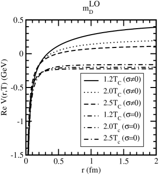
Figure 1: The real-part of the static potential with ($\sigma=0$) and without ($\sigma\neq 0$) non-perturbative term in the potential. The left (right) panel of the figure denote the results obtained with the leading-order and lattice-fitted Debye masses, respectively.

In the small-distance limit ($\hat{r}\ll 1$), the above potential reduces to the Cornell potential, i.e. the $Q\bar{Q}$-pair does not see the medium. On the other hand, in the long-distance limit ($\hat{r}\gg 1$), the potential is simplified into, with high temperature approximation (ie. $\sigma/m_{D}(T)$ can be neglected):

$${ReV_{(iso)}(r,T)}\approx-\frac{2\sigma}{m^{2}_{{}_{D}}r}-\alpha m_{{}_{D}},$$ (42)

which, apart from a constant term, is Coulomb-like potential by identifying $2\sigma/m_{{}_{D}}^{2}$ with the square of the strong coupling ($g^{2}$). However if we compare the asymptotic limit ($r\rightarrow\infty$) of our result (39) with the Digal et. al

$$F^{\rm{Digal}}(\infty,T) = \frac{\Gamma(1/4)}{2^{3/2}\Gamma(3/4)}\frac{\sigma}{m_{{D}}(T)}-\alpha m_{{D}}(T)$$

$$F^{\rm{Our}}(\infty,T) = \frac{2\sigma}{m_{{D}}(T)}-\alpha m_{{D}}(T),$$

the difference will be seen only in the string term only and may be due to the treatment of the problem classically or quantum mechanically. If we compare them quantitatively (with the Debye mass $m_{D}$= $1.4~{}m_{D}^{\rm{LO}}$), the difference becomes tiny.

To see the effect of the linear term on the potential, in addition to the Coulomb term, we have plotted the (real-part) potential (in Fig.1) with ($\sigma\neq 0$) and without string term ($\sigma=0$). We found that the inclusion of the linear term makes the potential attractive, compared to potential with the Coulomb term only. Furthermore, to see the effects of the screening scale, we have also computed the potential with the Debye mass in next-to-leading order (1.4$m_{D}^{\rm{LO}}$) which is seen less stronger than the leading-order result. To see the effects of medium on the potential at T=0, we have evaluated the potential at different temperatures viz. at $1.2T_{c}$, $2.0T_{c}$ and $2.5T_{c}$, where the potential is found to decrease with the temperature at large distances and becomes short-range. Thus the deconfinement is reflected clearly in the large-distance behavior of heavy quark potential at finite temperature, where the screening is operative. Thus the in-medium behavior of heavy quark bound states is used to probe the state of matter in QCD thermodynamics.

2.2.2 Imaginary Part of the Potential: Thermal Width, $\Gamma_{\rm{iso}}$

The imaginary part of the potential originates from the static limit of symmetric self energy. Cutting rules at finite temperature allows one to obtain the imaginary part by cutting open one of the hard thermal loop of the HTL propagator which represents physically the inelastic scattering of the off-shell gluon off a thermal gluon [10, 17, 36, 67], i.e. $g+(Q\bar{Q})\rightarrow g+Q+{\bar{Q}}$. The imaginary part of the potential plays an important role in weakening the bound state peak or transforming it to mere threshold enhancement. It leads to a finite width ($\Gamma$) for the resonance peak in the spectral function, which, in turn, determines the dissociation temperature. Dissociation is expected to occur while the (twice) binding energy decreases with the temperature and becomes equal to $\sim\Gamma$ [23, 35].

To obtain the imaginary part of the potential in isotropic medium, we write the temporal component of the symmetric propagator from (32) for $\xi=0$, in the static limit,

$$ImD^{00}_{F(iso)}(0,p)=\frac{-2\pi Tm_{D}^{2}}{p(p^{2}+m_{D}^{2})^{2}}.$$ (43)

However the same (43) could also be obtained for partons with space-like momenta ($p_{0}^{2}<p^{2}$) from the retarded (advanced) self energy (26), using the relation [17, 63]:

$$\ln\frac{p_{0}+p\pm i\epsilon}{p_{0}-p\pm i\epsilon}=\ln|\frac{p_{0}+p}{p_{0}-p}|\mp i\pi\theta(p^{2}-{p_{0}}^{2})~{}.$$ (44)

Thus the imaginary part of the symmetric propagator (43) gives the imaginary part of the dielectric function in isotropic medium :

$$\epsilon^{-1}(p)=-\pi Tm_{D}^{2}\frac{p^{2}}{p(p^{2}+m_{D}^{2})^{2}}.$$ (45)

One can then similarly find the imaginary part of the potential from the definition of potential (1)

$$ImV_{(iso)}(r,T) = -\int\frac{d^{3}\mathbf{p}}{(2\pi)^{3/2}}(e^{i\mathbf{p}\cdot\mathbf{r}}-1)\left(-\sqrt{\frac{2}{\pi}}\frac{\alpha}{p^{2}}-\frac{4\sigma}{\sqrt{2\pi}p^{4}}\right){p^{2}}\left[\frac{-\pi Tm_{D}^{2}}{p(p^{2}+m_{D}^{2})^{2}}\right]$$ (46)

$$\equiv ImV_{1(iso)}(r,T)+ImV_{2(iso)}(r,T)~{},$$

where $ImV_{1(iso)}(r,T)$ and $ImV_{2(iso)}(r,T)$ are the imaginary parts of the potential due to the medium modification to the short-distance and long-distance terms, respectively:

$$ImV_{1(iso)}(r,T) = -\frac{\alpha}{2\pi^{2}}\int d^{3}\mathbf{p}(e^{i\mathbf{p}\cdot\mathbf{r}}-1)\left[\frac{\pi Tm_{D}^{2}}{p(p^{2}+m_{D}^{2})^{2}}\right],$$

$$ImV_{2(iso)}(r,T) = -\frac{4\sigma}{({2\pi})^{2}}\int\frac{d^{3}{\bf p}}{(2\pi)^{3/2}}(e^{i{\bf p}\cdot{\bf r}}-1)\frac{1}{p^{2}}\left[\frac{\pi Tm_{D}^{2}}{p(p^{2}+m_{D}^{2})^{2}}\right].$$ (47)

After performing the integration, the contribution due to the short-distance term to imaginary part becomes (with $z=p/m_{D}$)

$$ImV_{1(iso)}({\bf r},T) = -2\alpha T\int_{0}^{\infty}\frac{dz}{(z^{2}+1)^{2}}\left(1-\frac{\sin{z\hat{r}}}{z\hat{r}}\right)$$ (48)

$$\equiv -\alpha T\phi_{0}(\hat{r}),$$

and the contribution due to the string term becomes

$$ImV_{2(iso)}(r,T) = \frac{4\sigma T}{m_{D}^{2}}\int_{0}^{\infty}\frac{dz}{z(z^{2}+1)^{2}}\left(1-\frac{\sin{z\hat{r}}}{z\hat{r}}\right)$$ (49)

$$\equiv \frac{2\sigma T}{m_{D}^{2}}\psi_{0}(\hat{r})~{},$$

where the functions, $\phi_{0}(\hat{r})$ and $\psi_{0}(\hat{r})$ at leading-order in $\hat{r}$ are

$$\phi_{0}(\hat{r})=-\alpha T\left(-\frac{{\hat{r}}^{2}}{9}\left(-4+3\gamma_{E}+3\log\hat{r}\right)\right)$$ (50)

$$\psi_{0}(\hat{r})=\frac{\hat{r}^{2}}{6}+\left(\frac{-107+60\gamma_{E}+60\log(\hat{r})}{3600}\right)\hat{r}^{4}+O(\hat{r}^{5}).$$ (51)

In the short-distance limit ($\hat{r}\ll 1$), both the contributions, at the leading logarithmic order, reduce to

$$ImV_{1(iso)}(r,T)=-\alpha T\frac{{\hat{r}^{2}}}{3}\log(\frac{1}{\hat{r}}),$$ (52)

$$ImV_{2(iso)}(r,T)=-\frac{2\sigma T}{m_{D}^{2}}\frac{{\hat{r}^{4}}}{60}\log(\frac{1}{\hat{r}}),$$ (53)

thus the sum of Coulomb and string term gives the imaginary part of the potential in isotropic medium:

$$ImV_{\rm{(iso)}}(r,\xi,T)=-T\left(\frac{\alpha{\hat{r}^{2}}}{3}+\frac{\sigma{\hat{r}}^{4}}{30m_{D}^{2}}\right)\log(\frac{1}{\hat{r}}).$$ (54)

One thus immediately observes that for small distances the imaginary part vanishes and its magnitude is larger than the case where only the Coulombic term is considered [69] and thus enhances the width of the resonances in thermal medium.

The imaginary part of the potential, in small-distance limit, is a perturbation to the vacuum potential and thus provides an estimate for the width ($\Gamma$) for a resonance state and can be calculated, in a first-order perturbation, by folding with the unperturbed (1S) Coulomb wavefunction

$$\Gamma_{\rm{(iso)}}=\left(\frac{4T}{\alpha m_{Q}^{2}}+\frac{12\sigma T}{\alpha^{2}m_{Q}^{4}}\right)~{}m_{D}^{2}~{}\log\frac{\alpha m_{Q}}{2m_{D}}.$$ (55)

The main features of our results on the thermal width in (Fig.2) are: First the width always increases with the temperature. Secondly the inclusion of the non vanishing nonperturbative string term, in addition to the Coulomb term, makes the width larger than the earlier result with the perturbative Coulomb term [85] only and thus the damping of the exchanged gluon in the heat bath provides larger contribution to the dissociation rate and consequently reduce the yield of dileptons in the peak.

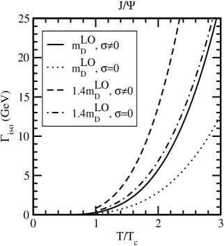
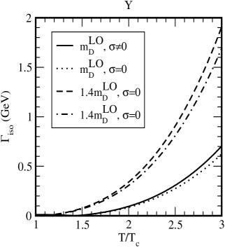
Figure 2: Decay width of $J/\psi$ (left) and $\Upsilon$ (right) states with and without nonperturbative (string) term in an isotropic medium with the Debye masses in leading-order and the lattice fitted result.

The effect of nonperturbative term on the width is relatively more on $J/\psi$ than $\Upsilon$ state because the binding of $\Upsilon$ (1S) state is more Coulombic than $J/\psi$ (1S) state. This may have far reaching implications on the dissociation in medium. Thirdly the width is also affected by the screening scale we chose to regulate the potential, namely the width with the higher screening scale (1.4 $m_{D}^{\rm{LO}}$) is more than the leading-order result because the width, $\Gamma$ increases with the increase of the Debye mass.

2.2.3 Real and Imaginary Binding Energies: Dissociation Temperatures

To understand the in-medium properties of the quarkonium states, one need to solve the Schrödinger equation with both the real and imaginary part of the finite temperature potential. As seen earlier, in the short-distance limit, the vacuum contribution dominates over the medium contribution whereas in the long-distance limit the real part of the potential reduces to a Coulomb like potential and thus yields the real part of the binding energy in isotropic medium:

$$\rm{Re}~{}E_{\rm{bin}}^{\rm{iso}}\stackrel{{\scriptstyle\hat{r}\gg 1}}{{=}}\left(\frac{m_{Q}\sigma^{2}}{m_{{}_{D}}^{4}n^{2}}+\alpha m_{{}_{D}}\right);~{}n=1,2\cdot\cdot\cdot$$ (56)

However in the intermediate-distance ($rm_{D}\simeq 1$) scale, the interaction becomes complicated and the potential does not look simpler in contrast to the asymptotic limits, thus the complex potential in general needs to be dealt with numerically to obtain the real and imaginary binding energies. There are some numerical methods to solve the Schrödinger equation either in partial differential form (time-dependent) or eigen value form (time-independent) by the finite difference time domain method (FDTD) or matrix method, respectively. In the later method, the stationary Schrödinger equation can be solved in a matrix form through a discrete basis, instead of the continuous real-space position basis spanned by the states $|\overrightarrow{x}\rangle$. Here the confining potential V is subdivided into N discrete wells with potentials $V_{1},V_{2},...,V_{N+2}$ such that for $i^{\rm{th}}$ boundary potential, $V=V_{i}$ for $x_{i-1}<x<x_{i};~{}i=2,3,...,(N+1)$. Therefore for the existence of a bound state, there must be exponentially decaying wave function in the region $x>x_{N+1}$ as $x\rightarrow\infty$ and has the form:

$$\Psi_{N+2}(x)=P_{{}_{E}}\exp[-\gamma_{{}_{N+2}}(x-x_{N+1})]+Q_{{}_{E}}\exp[\gamma_{{}_{N+2}}(x-x_{N+1})],$$ (57)

where, $P_{{}_{E}}=\frac{1}{2}(A_{N+2}-B_{N+2})$, $Q_{{}_{E}}=\frac{1}{2}(A_{N+2}+B_{N+2})$ and, $\gamma_{{}_{N+2}}=\sqrt{2\mu(V_{N+2}-E)}$. The eigenvalues can be obtained by identifying the zeros of $Q_{E}$.

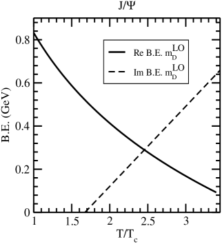
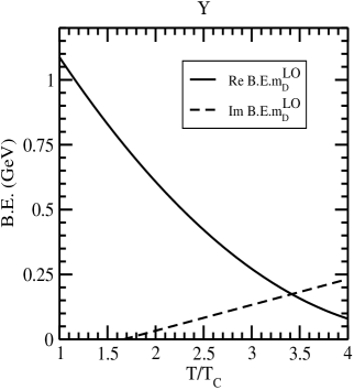
Figure 3: Variation of the real and imaginary binding energies for the $J/\psi$ and $\Upsilon$ states with the temperature (in units of critical temperature, $T_{c}$) in the left and right panel, respectively in an isotropic medium.

The binding energies shown in Fig. 3 have the following features: First when the nonperturbative term is included, the (real part) binding of $Q\bar{Q}$ pairs gets stronger with respect to the case where only the Coulomb term is included. Secondly there is a strong decreasing trend with the temperature because the screening becomes stronger with the increase of the temperature, so the real part of the potential becomes weaker compared to $T=0$ and results in early dissolution of quarkonia in the medium. Thirdly the real part of the binding energy decreases with the increase of screening scale (1.4 $m_{D}^{\rm{LO}}$). On the other hand the imaginary part of the binding energy increases with the temperature. Thus the study of both the binding energies is poised to provide a wealth of information about the dissociation pattern of quarkonium states in thermal medium which will be used to determine the dissociation temperatures.

We will now study the dissociation in thermal medium to calculate the dissociation temperature ($T_{d}$) either from the intersection of the (real and imaginary) binding energies  [46, 65], or from the conservative criterion on the width of the resonance as: $\Gamma\geq 2\rm{Re}~{}{\rm{B.E.}}$ [23]. Although both definitions are physically equivalent but they are numerically different (Table 1). For example, $J/\psi$ is dissociated at 2.45 $T_{c}$ obtained from the intersection of binding energies while the condition on width gives much lower temperature (1.40 $T_{c}$) . Correspondingly $\Upsilon$ (1S) is dissociated at 3.40 $T_{c}$ and 3.10 $T_{c}$, respectively. Our results are found relatively higher compared to similar calculation [46, 65], which may be due to the absence of three-dimensional medium modification of the linear term in their calculation.

Finally we explore the sensitivity of the screening scale on the dissociation mechanism where the dissociation temperatures computed with the next-to-leading order (1.4 $m_{D}^{\rm{LO}}$) Debye mass are found smaller than the leading-order result (Table 2). For example, $J/\psi$’s and $\Upsilon$’s are now dissociated at 1.33 $T_{c}$ and 1.91$T_{c}$, respectively.

2.3 Potential in the anisotropic medium

The space-time evolution of QGP relys on the viscous hydrodynamical treatment where the system assumes a local thermal equilibrium, i.e. close to isotropic in momentum space, which may not be true at the very early time in the collision of two nuclei, due to large momentum-space anisotropies [78, 86, 87]. The degree of anisotropy increases as the shear viscosity increases and thus one must address it while calculating the heavy quark potential in the presence of momentum-space anisotropies. The real-part of the heavy quark potential was first considered in [61] and then the imaginary part was obtained theoretically [63, 64, 88] as well as phenomenologically [46, 62, 65]. The main effect of the anisotropy is to reduce Debye screening which, in turn has the effect that heavy quarkonium states can survive upto higher temperatures. However the aforesaid works in anisotropic medium are limited to the medium-modification of the perturbative part only and the nonperturbative string term was assumed to zero. However, the string-tension is non vanishing even at temperatures much beyond the deconfinement point [53, 54, 55], so one should study its effect on the heavy quark potential in anisotropic medium too.

2.3.1 Real Part of the Potential

Like in isotropic medium, we obtain the real-part of the potential in weakly-anisotropic medium [66] from the anisotropic corrections to the (temporal component) real-part of retarded propagator (31)

$$ReV_{\rm(aniso)}({\bf r},\xi,T) = \int\frac{d^{3}\mathbf{p}}{{(2\pi)}^{3/2}}(e^{i\mathbf{p}\cdot\mathbf{r}}-1)\left(-\sqrt{(2/\pi)}\frac{\alpha}{p^{2}}-\frac{4\sigma}{\sqrt{2\pi}p^{4}}\right)\times$$ (58)

$$p^{2}\left[\frac{1}{(p^{2}+m_{D}^{2})}-\frac{\xi m_{D}^{2}}{6(p^{2}+m_{D}^{2})^{2}}(3\cos(2\theta_{p})-1)\right]$$

$$\equiv ReV_{1(aniso)}({\bf r},\xi,T)+ReV_{2(aniso)}({\bf r},\xi,T)~{},$$

where $ReV_{1(aniso)}({\bf r},\xi,T)$ and $ReV_{2(aniso)}(\mathbf{r},\xi,T)$ are the medium modifications corresponding to the Coulomb and string term, respectively, are given by

$$ReV_{1(aniso)}({\bf r},\xi,T) = -\frac{\alpha}{2\pi^{2}}\int d^{3}\mathbf{p}(e^{i\mathbf{p}\cdot\mathbf{r}}-1)\left[\frac{1}{(p^{2}+m_{D}^{2})}-\frac{\xi m_{D}^{2}}{6(p^{2}+m_{D}^{2})^{2}}(3\cos 2\theta_{p}-1)\right]$$ (59)

$$ReV_{2(aniso)}({\bf r},\xi,T) = -\frac{4\sigma}{{2\pi}^{2}}\int d^{3}\mathbf{p}(e^{i\mathbf{p}\cdot\mathbf{r}}-1)\frac{1}{p^{2}}\left[\frac{1}{(p^{2}+m_{D}^{2})}-\frac{\xi m_{D}^{2}}{6(p^{2}+m_{D}^{2})^{2}}(3\cos 2\theta_{p}-1)\right]~{}.$$ (60)

To perform the momentum integration, we use the transformation $\cos\theta_{p}=\cos\theta_{r}\cos\theta_{pr}+\sin\theta_{r}\sin\theta_{pr}\cos\phi_{pr}$, where $\theta_{p}$ and $\theta_{r}$ are the angles between p and n, r and n, respectively and $\theta_{pr}$, $\phi_{pr}$ are the angular variables between the vectors, ${\bf p}$ and ${\bf r}$. So after the integration, the Coulombic contribution to the potential becomes

$$ReV_{1(aniso)}({\bf r},\xi,T) = -\alpha m_{D}\left[\frac{e^{-\hat{r}}}{\hat{r}}+1+\xi\left[\frac{(e^{-\hat{r}}-1)}{6}+\left[e^{-\hat{r}}\left(\frac{1}{6}+\frac{1}{2\hat{r}}+\frac{1}{\hat{r}^{2}}\right)+\frac{(e^{-\hat{r}}-1)}{\hat{r}^{3}}\right]\right.\right.\times$$ (61)

$$\left.\left.(1-3\cos^{2}\theta_{r})\right]\right]~{},$$

and the string contribution is

$$ReV_{2(aniso)}({\bf r},\xi,T) = \frac{2\sigma}{m_{{}_{D}}}\left[\frac{(e^{-\hat{r}}-1)}{\hat{r}}+1+2\xi\left[\left(\frac{(e^{-\hat{r}}-1)}{6\hat{r}}+\frac{e^{-\hat{r}}}{12}+\frac{1}{6}\right)\right.\right.$$ (62)

$$\left.\left.+\left(e^{-\hat{r}}\left(\frac{1}{{\hat{r}}^{2}}+\frac{5}{12\hat{r}}+\frac{1}{12}\right)+\frac{1}{12\hat{r}}+\frac{(e^{-\hat{r}}-1)}{{\hat{r}}^{3}}\right)(1-3\cos^{2}\theta_{r})\right]\right]~{}.$$

Thus the real-part of the potential in the anisotropic medium becomes

$$ReV_{aniso}(r,\theta_{r},T) = \left(\frac{2\sigma}{m_{{}_{D}}}-\alpha m_{{}_{D}}\right)\frac{e^{-\hat{r}}}{\hat{r}}-\frac{2\sigma}{m_{{}_{D}}\hat{r}}+\frac{2\sigma}{m_{{}_{D}}}-\alpha m_{{}_{D}}$$ (63)

$$+ \xi\left(\frac{2\sigma}{m_{D}}\frac{e^{-\hat{r}}}{\hat{r}}\left[\frac{e^{\hat{r}}-1}{\hat{r}^{2}}-\frac{5e^{\hat{r}}}{12}+\frac{\hat{r}e^{\hat{r}}}{3}-\frac{1}{\hat{r}}+\frac{\hat{r}}{12}-\frac{1}{12}\right]\right.$$

$$- \left.\frac{\alpha m_{D}}{2}\frac{e^{-\hat{r}}}{\hat{r}}\left[\frac{e^{\hat{r}}-1}{\hat{r}^{2}}-\frac{1}{\hat{r}}-\frac{\hat{r}e^{\hat{r}}}{3}+\frac{\hat{r}}{6}-\frac{1}{2}\right]\right.$$

$$+ \left(\left.\frac{2\sigma}{m_{D}}\frac{e^{-\hat{r}}}{\hat{r}}\left[3\frac{e^{\hat{r}}-1}{\hat{r}^{2}}-\frac{e^{\hat{r}}}{4}-\frac{3}{\hat{r}}-\frac{\hat{r}}{4}-\frac{5}{4}\right]\right.\right.$$

$$- \frac{\alpha m_{D}}{2}\frac{e^{-\hat{r}}}{\hat{r}}\left[\left.\left.3\frac{e^{\hat{r}}-1}{\hat{r}^{2}}-\frac{3}{\hat{r}}-\frac{\hat{r}}{2}-\frac{3}{2}\right]\right)\cos~{}2\theta_{r}\right)$$

$$= ReV_{iso}(r,T)+V_{\rm{tensor}}(r,\theta_{r},T).$$

Thus the anisotropy in the momentum space introduces an angular ($\theta_{r}$) dependence, in addition to the interparticle separation ($r$), to the real part of the potential, in contrast to the $r$-dependence only in an isotropic medium. The real potential becomes stronger with the increase of anisotropy (shown in Fig.4) because the (anisotropic) Debye mass $m_{D}(\xi,T)$ (or equivalently angular-dependent Debye mass $m_{D}(\theta_{r},T)$) in an anisotropic medium is always smaller than in an isotropic medium. As a result the screening of the Coulomb and string contribution are less accentuated, compared to the isotropic medium. In particular the potential for quark pairs aligned in the direction of anisotropy are stronger than the pairs aligned in the transverse direction.

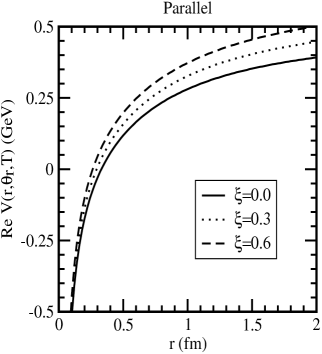
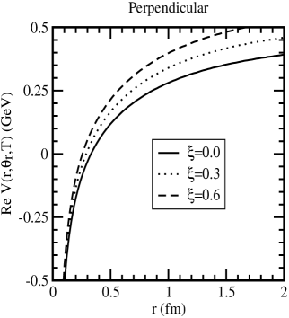
Figure 4: Real part of the potential for both the parallel (left)and perpendicular (right) alignment with the Debye mass in the leading-order.

2.3.2 Imaginary Part of the Potential: Thermal width, $\Gamma_{\rm{aniso}}$

Recently the imaginary part with a momentum-space anisotropy and its effects on the thermal widths of the resonance states have been studied [65, 69, 85, 89], with the medium-modification to the perturbative (Coulomb) term only. The imaginary part of the potential arises due to the singlet-to-octet transitions induced by the dipole vertex as well as due to the Landau damping in the plasma, i.e. scattering of the gluons with space-like momentum off the thermal excitations in the medium. We follow their work by including the medium corrections to both perturbative (Coulombic) and non-perturbative (string) terms in a weakly anisotropic medium. Like in isotropic medium, we can obtain the imaginary part of the potential by the leading anisotropic correction to the imaginary part of the (temporal component) symmetric propagator as

$$ImV_{\rm(aniso)}({\bf r},\xi,T) = -\int\frac{d^{3}\mathbf{p}}{(2\pi)^{3/2}}(e^{i\mathbf{p}\cdot\mathbf{r}}-1)\left(-\sqrt{\frac{2}{\pi}}\frac{\alpha}{p^{2}}-\frac{4\sigma}{\sqrt{2\pi}p^{4}}\right)p^{2}\left[\frac{-\pi Tm_{D}^{2}}{p(p^{2}+m_{D}^{2})^{2}}\right.$$ (64)

$$\left.+\xi[\frac{3\pi Tm_{D}^{2}}{2p(p^{2}+m_{D}^{2})^{2}}\sin^{2}{\theta_{p}}-\frac{4\pi Tm_{D}^{4}}{p(p^{2}+m_{D}^{2})^{3}}(\sin^{2}\theta_{p}-\frac{1}{3})\right]$$

$$\equiv ImV_{1(aniso)}({\bf r},\xi,T)+ImV_{2(aniso)}({\bf r},\xi,T)~{},$$

where $ImV_{1(aniso)}({\bf r},\xi,T)$ and $ImV_{2(aniso)}(\mathbf{r},\xi,T)$ are the imaginary contributions corresponding to the Coulombic and linear terms in anisotropic medium, respectively:

$$ImV_{1\rm(aniso)}({\bf r},\xi,T) = \frac{\alpha}{2\pi^{2}}\int d^{3}\mathbf{p}(e^{i\mathbf{p}\cdot\mathbf{r}}-1)\left[\frac{-\pi Tm_{D}^{2}}{p(p^{2}+m_{D}^{2})^{2}}+\xi\left[\frac{3\pi Tm_{D}^{2}}{4p(p^{2}+m_{D}^{2})^{2}}\sin^{2}{\theta_{p}}\right.\right.$$ (65)

$$\left.\left.-\frac{2\pi Tm_{D}^{4}}{p(p^{2}+m_{D}^{2})^{3}}(\sin^{2}\theta_{p}-\frac{1}{3})\right]\right],$$

$$ImV_{2\rm(aniso)}({\bf r},\xi,T) = \frac{4\sigma}{({2\pi})^{2}}\int\frac{d^{3}\mathbf{p}}{(2\pi)^{3/2}}(e^{i\mathbf{p}\cdot\mathbf{r}}-1)\frac{1}{p^{2}}\left[\frac{-\pi Tm_{D}^{2}}{p(p^{2}+m_{D}^{2})^{2}}+\xi\left[\frac{3\pi Tm_{D}^{2}}{4p(p^{2}+m_{D}^{2})^{2}}\sin^{2}{\theta_{p}}\right.\right.$$

$$\left.\left.-\frac{2\pi Tm_{D}^{4}}{p(p^{2}+m_{D}^{2})^{3}}(\sin^{2}\theta_{p}-\frac{1}{3})\right]\right].$$ (66)

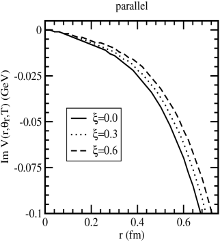
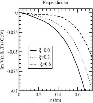
Figure 5: Imaginary part of the potential for parallel (left) and perpendicular (Right) alignment in an anisotropic medium.

Since the isotropic contribution is already calculated in Sec.2.2.2, so the anisotropic contribution to the perturbative term in the leading-order is given by [69]

$$ImV_{1(aniso)}({\bf r},\xi,T) \equiv \alpha T\xi\left[\phi_{1}(\hat{r},\theta_{r})+\phi_{2}(\hat{r},\theta_{r})\right],$$ (67)

where the functions $\phi_{1}(\hat{r},\theta_{r})$ and $\phi_{2}(\hat{r},\theta_{r})$ are

$$\phi_{1}(\hat{r},\theta_{r}) = \frac{{\hat{r}}^{2}}{600}\left[123-90\gamma_{E}-90\log\hat{r}+\cos(2\theta_{r})\left(-31+30\gamma_{E}+30\log\hat{r}\right)\right],$$

$$\phi_{2}(\hat{r},\theta_{r}) = \frac{{\hat{r}}^{2}}{90}(-4+3\cos(2\theta_{r})).$$ (68)

Similarly the imaginary contribution due to the nonperturbative (linear) term can also separated into the isotropic and anisotropic term, where the isotropic part is already calculated in Sec.2.2.2 and hence the anisotropic part is now calculated

$$ImV_{2(aniso)}(r,\xi,T)=-\xi~{}\frac{2\sigma T}{m_{D}^{2}}\left[\psi_{1}(\hat{r},\theta_{r})+\psi_{2}(\hat{r},\theta_{r})\right]~{}.$$ (69)

The function, $\psi_{1}(\hat{r},\theta_{r})$ is given by

$$\psi_{1}(\hat{r},\theta_{r}) = \int\frac{dz}{z(z^{2}+1)^{2}}\left[1-\frac{3}{2}\left(\sin^{2}\theta_{r}\frac{\sin{z\hat{r}}}{z\hat{r}}+(1-3\cos^{2}\theta_{r})G(\hat{r},z)\right)\right]~{},$$ (70)

where $G(\hat{r},z)$ is given by

$$G(\hat{r},z) = \frac{z\hat{r}\cos(z\hat{r})-\sin(z\hat{r})}{(z\hat{r})^{3}}.$$ (71)

Substituting $G(\hat{r},z)$ into $\psi_{1}(\hat{r},\theta_{r})$ and decomposing into $\theta_{r}$- dependent and independent terms, the function, $\psi_{1}(\hat{r},\theta_{r})$ can be rewritten as

$$\psi_{1}(\hat{r},\theta_{r}) = \int\frac{dz}{z(z^{2}+1)^{2}}\left[1-\frac{3}{2}\left(\frac{\sin(z\hat{r})}{z\hat{r}}+\frac{\cos(z\hat{r})}{(z\hat{r})^{2}}-\frac{\sin(z\hat{r})}{(z\hat{r})^{3}}\right)\right.$$ (72)

$$\left.+\frac{3}{2}\left(\frac{\sin(z\hat{r})}{z\hat{r}}+3\frac{\cos(z\hat{r})}{(z\hat{r})^{2}}-3\frac{\sin(z\hat{r})}{(z\hat{r})^{3}}\right)\cos^{2}\theta_{r})\right]$$

$$\equiv \psi_{1}^{(1)}(\hat{r})+\psi_{1}^{(2)}(\hat{r},\theta_{r})~{},$$

where the functions $\psi_{1}^{(1)}(\hat{r})$ and $\psi_{1}^{(2)}(\hat{r},\theta_{r})$ are given by

$$\psi_{1}^{(1)}(\hat{r}) = \int\frac{dz}{z(z^{2}+1)^{2}}\left[1-\frac{3}{2}\left(\frac{\sin(z\hat{r})}{z\hat{r}}+\frac{\cos(z\hat{r})}{(z\hat{r})^{2}}-\frac{\sin(z\hat{r})}{(z\hat{r})^{3}}\right)\right]$$ (73)

$$= \hat{r}^{4}\int\frac{dx}{x(x^{2}+\hat{r}^{2})^{2}}\left[1-\frac{3}{2}\left(\frac{\sin(x)}{x}+\frac{\cos(x)}{x^{2}}-\frac{\sin(x)}{x^{3}}\right)\right]$$

$$= \frac{\hat{r}^{2}}{10}+\frac{(-739+420\gamma_{E}+420\log(\hat{r}))\hat{r}^{4}}{39200}+O(\hat{r}^{5}),$$

and

$$\psi_{1}^{(2)}(\hat{r},\theta_{r}) = \frac{3}{2}\int\frac{dz}{z(z^{2}+1)^{2}}\left[\left(\frac{\sin(z\hat{r})}{z\hat{r}}+3\frac{\cos(z\hat{r})}{(z\hat{r})^{2}}-3\frac{\sin(z\hat{r})}{(z\hat{r})^{3}}\right)\cos^{2}\theta_{r})\right]$$ (74)

$$= \frac{3}{2}\hat{r}^{4}\int\frac{dx}{x(x^{2}+\hat{r}^{2})^{2}}\left[\left(\frac{\sin(x)}{x}+\frac{3\cos(x)}{x^{2}}-\frac{3\sin(x)}{x^{3}}\right)\cos^{2}\theta_{r}\right]$$

$$= \left(-\frac{r^{2}}{20}+\frac{(176-105\gamma_{E}-105\log(\hat{r}))\hat{r}^{4}}{14700}+O(\hat{r}^{5})\right)\cos^{2}\theta_{r}~{}.$$

The remaining function in the imaginary part of the potential associated with the linear term (69) can similarly be separated into $\theta_{r}$- dependent and independent terms:

$$\psi_{2}(\hat{r},\theta_{r}) = -\frac{4}{3}\int\frac{dz}{z(z^{2}+1)^{3}}\left[1-3\left[(\frac{2}{3}-\cos^{2}\theta_{r})\frac{\sin{z\hat{r}}}{z\hat{r}}+(1-3\cos^{2}\theta_{r})G(\hat{r},z)\right]\right]$$ (75)

$$= -\frac{4}{3}\int\frac{dz}{z(z^{2}+1)^{3}}\left[\left(1-\frac{2\sin{z\hat{r}}}{z\hat{r}}-\frac{3\cos(z\hat{r})}{(z\hat{r})^{2}}+\frac{3\sin(z\hat{r})}{(z\hat{r})^{3}}\right)\right.$$

$$\left.+3\left(\frac{\sin{z\hat{r}}}{z\hat{r}}+\frac{3\cos(z\hat{r})}{(z\hat{r})^{2}}-\frac{3\sin(z\hat{r})}{(z\hat{r})^{3}}\right)\cos^{2}\theta_{r}\right]$$

$$\equiv \psi_{2}^{(1)}(\hat{r})+\psi_{2}^{(2)}(\hat{r},\theta_{r}),$$

where the functions $\psi_{2}^{(1)}(\hat{r})$ and $\psi_{2}^{(2)}(\hat{r},\theta_{r})$ are given by

$$\psi_{2}^{(1)}(\hat{r}) = -\frac{4}{3}\int\frac{dz}{z(z^{2}+1)^{3}}\left(1-\frac{2\sin{z\hat{r}}}{z\hat{r}}-\frac{3\cos(z\hat{r})}{(z\hat{r})^{2}}+\frac{3\sin(z\hat{r})}{(z\hat{r})^{3}}\right)$$ (76)

$$= -\frac{4}{3}\left[\frac{7\hat{r}^{2}}{120}-\frac{11\hat{r}^{4}}{3360}+O(\hat{r}^{5})\right],$$

and

$$\psi_{2}^{(2)}(\hat{r},\theta_{r}) = -4\int\frac{dz}{z(z^{2}+1)^{3}}\left(\frac{\sin{z\hat{r}}}{z\hat{r}}+\frac{3\cos(z\hat{r})}{(z\hat{r})^{2}}-\frac{3\sin(z\hat{r})}{(z\hat{r})^{3}}\right)\cos^{2}\theta_{r}$$ (77)

$$= -4\left[-\frac{\hat{r}^{2}}{60}+\frac{\hat{r}^{4}}{840}+O(\hat{r}^{5})\right]\cos^{2}\theta_{r}.$$

So the functions $\psi_{1}(\hat{r},\theta_{r})$ and $\psi_{2}(\hat{r},\theta_{r})$ are finally given by

$$\psi_{1}(\hat{r},\theta_{r}) = \frac{\hat{r}^{2}}{10}+\frac{(-739+420\gamma_{E}+420\log(\hat{r}))\hat{r}^{4}}{39200}$$ (78)

$$+ \left(-\frac{\hat{r}^{2}}{20}+\frac{(176-105\gamma_{E}-105\log(\hat{r}))\hat{r}^{4}}{14700}\right)\cos^{2}\theta_{r},$$

$$\psi_{2}(\hat{r},\theta_{r}) = -\frac{4}{3}\left[\frac{7\hat{r}^{2}}{120}-\frac{11\hat{r}^{4}}{3360}+O(\hat{r}^{5})\right]$$ (79)

$$-4\left[-\frac{\hat{r}^{2}}{60}+\frac{\hat{r}^{4}}{840}+O(\hat{r}^{5})\right]\cos^{2}\theta_{r}~{},$$

respectively and $\gamma_{E}$ is the Euler-Gamma constant.

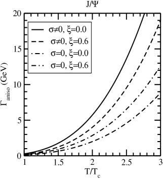
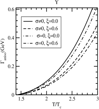
Figure 6: The thermal width for the $J/\psi$ and $\Upsilon$ states in the anisotropic medium.

Finally the short and long-distance contributions, in the leading logarithmic order

$$ImV_{1(aniso)}(r,\theta_{r},T) = -\alpha T{\hat{r}^{2}}\log(\frac{1}{\hat{r}})\left(\frac{1}{3}-\xi\frac{3-\cos 2\theta_{r}}{20}\right),$$ (80)

$$ImV_{2(aniso)}(r,\theta_{r},T) = -\frac{2\sigma T}{m_{D}^{2}}\frac{\hat{r}^{4}}{20}\log(\frac{1}{\hat{r}})\left(\frac{1}{3}-\xi\frac{2-\cos 2\theta_{r}}{14}\right)~{},$$ (81)

gives the imaginary part of the potential in the anisotropic medium

$$ImV_{\rm{(aniso)}}(r,\theta_{r},T) = -T\left(\frac{\alpha{\hat{r}^{2}}}{3}+\frac{\sigma{\hat{r}}^{4}}{30m_{D}^{2}}\right)\log(\frac{1}{\hat{r}})$$ (82)

$$+\xi T\left[\left(\frac{\alpha{\hat{r}^{2}}}{5}+\frac{3\sigma{\hat{r}^{4}}}{140m_{D}^{2}}\right)\right.\left.-\cos^{2}\theta_{r}\left(\frac{\alpha{\hat{r}^{2}}}{10}+\frac{\sigma{\hat{r}^{4}}}{70m_{D}^{2}}\right)\right]\log(\frac{1}{\hat{r}})~{},$$

which is found to be smaller than the isotropic medium and decreases with the increase of anisotropy (shown in Fig.5).

Method	State	$\xi=0.0$	$\xi=0.3$	$\xi=0.6$
Re B.E.=Im B.E.	$J/\psi$	2.45	2.46	2.47
	$\Upsilon$	3.40	3.45	3.46
$\Gamma$=2B.E.	$J/\psi$	1.40	1.46	1.54
	$\Upsilon$	3.10	3.17	3.26

Table 1: Dissociation temperatures of $J/\psi$ and $\Upsilon$ states for different anisotropies with the Debye mass in leading-order.

Method	State	$\xi=0.0$	$\xi=0.3$	$\xi=0.6$
Re B.E.=Im B.E.	$J/\psi$	1.33	1.34	1.35
	$\Upsilon$	1.91	1.93	1.94
$\Gamma$=2B.E.	$J/\psi$	1.02	1.06	1.12
	$\Upsilon$	1.88	1.92	2.02

Table 2: The same as Table 1, having the Debye mass ($m_{D}=1.4~{}m_{D}^{\rm{LO}}$)

Like in isotropic medium, in weakly anisotropic medium too, the imaginary part is found to be a perturbation and thus provides an estimate for the (thermal) width for a particular resonance state:

$$\Gamma_{\rm(aniso)} = \int d^{3}{\bf r}|\Psi(r)|^{2}\left[\alpha T{\hat{r}^{2}}\log(\frac{1}{\hat{r}})\left(\frac{1}{3}-\xi\frac{3-\cos 2\theta_{r}}{20}\right)\right.$$ (83)

$$\left.+\frac{2\sigma T}{m_{D}^{2}}{\hat{r}^{4}}\log(\frac{1}{\hat{r}})\frac{1}{20}\left(\frac{1}{3}-\xi\frac{2-\cos 2\theta_{r}}{14}\right)\right]$$

$$= T\left(\frac{4}{\alpha m_{Q}^{2}}+\frac{12\sigma}{\alpha^{2}m_{Q}^{4}}\right)\left(1-\frac{\xi}{2}\right)m_{D}^{2}\log\frac{\alpha m_{Q}}{2m_{D}}~{},$$

which shows that the width in anisotropic medium becomes smaller than in isotropic medium and gets narrower with the increase of anisotropy (shown in Fig. 6). This is due to the fact that $\Gamma$ is approximately proportional to the (square) Debye mass and the Debye mass decreases in the anisotropic medium because the effective local parton density around a test (heavy) quark is smaller compared to isotropic medium.

2.3.3 Real and Imaginary Binding Energies: Dissociation temperatures

The real part of the potential thus obtained in anisotropic medium (63), in contrast to its counterpart (spherically symmetric potential) in isotropic medium eq. (41) is non-spherical and so one cannot simply obtain the energy eigen values by solving the radial part of the Schrödinger equation alone because the radial part is no longer sufficient due to the angular dependence in the potential. Other way to understand is that because of the anisotropic screening scale, the wave functions are no longer radially symmetric for $\xi\neq 0$. So one has to solve the potential in three dimension but in the small $\xi$-limit, the non-symmetric component $V_{\rm{tensor}}(r,\theta_{r},T)$ is much smaller than the symmetric (isotropic) component $ReV_{\rm(iso)}(r,T)$ and thus can be treated as perturbation.

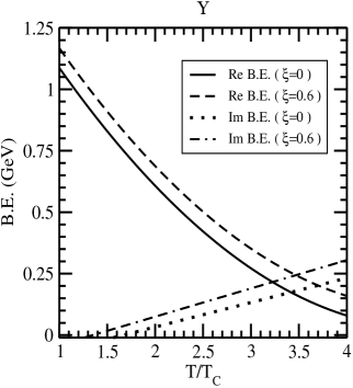
Figure 7: Variation of the real and imaginary part of the binding energies for $J/\psi$ and $\Upsilon$ states for different anisotropies.

Therefore, the corrected energy eigen values come from the solution of Schrödinger equation of the isotropic component plus the first-order perturbation due to the anisotropic component $V_{\rm{tensor}}(r,\theta_{r},T)$.

In short-distance limit, the vacuum contribution dominates over the medium contribution even for the weakly anisotropic medium and in the long-distance limit, the real part of potential in high temperature approximation results a Coulomb plus a subleading anisotropic contribution :

$$ReV_{\rm{(aniso)}}(r,\theta_{r},T) \stackrel{{\scriptstyle\hat{r}\gg 1}}{{\simeq}} -\frac{2\sigma}{m^{2}_{{}_{D}}r}-\alpha m_{{}_{D}}-\frac{5\xi}{12}~{}\frac{2\sigma}{m^{2}_{{}_{D}}r}\left(1+\frac{3}{5}\cos 2\theta_{r}\right)$$ (84)

$$\equiv ReV_{\rm{iso}}(\hat{r}\gg 1,T)+V_{\rm{tensor}}(\hat{r}\gg 1~{}.\theta_{r},T)~{}.$$ (85)

where the anisotropic contribution ($V_{\rm{tensor}}(\hat{r}\gg 1,\theta_{r},T)$) is smaller than the isotropic one ($ReV_{\rm{iso}}(\hat{r}\gg 1,T)$), so the anisotropic part can be treated as perturbation. Therefore, the real part of binding energy may be obtained from the radial part of the Schrödinger equation (of the isotropic component) plus the first-order perturbation due to the anisotropic component as

$${\rm Re}~{}E_{\rm{bin}}^{\rm{aniso}}=\left(\frac{m_{Q}\sigma^{2}}{m_{{}_{D}}^{4}n^{2}}+\alpha m_{{}_{D}}\right)+\frac{2\xi}{3}\frac{m_{Q}\sigma^{2}}{m_{{}_{D}}^{4}n^{2}},$$ (86)

where the first term is the solution of (radial-part) of the Schrödinger equation with the isotropic part ($ReV_{\rm{iso}}(\hat{r}\gg 1,T)$) and the second term is due to the anisotropic perturbation of the tensorial component ($V_{\rm{tensor}}(\hat{r}\gg 1,\theta_{r},T)$) calculated from the first-order perturbation theory.

The real and imaginary part of the binding energies for the $J/\psi$ and $\Upsilon$ states are computed numerically in Fig. 7 for different values of anisotropies, with the following observations: The inclusion of the nonperturbative string term makes the quarkonium states more bound in the anisotropic medium too. Secondly the binding of $Q\bar{Q}$ pairs becomes stronger with respect to their isotropic counterpart and increases with the increase of anisotropy because the (real part) potential becomes deeper due to the weaker screening. Last but not the least, as the screening scale increases the binding gets weakened even in the anisotropic medium. In contrast to the real part of binding energy, the imaginary part of the binding energy increases with the temperature but increases with the anisotropy. With these observations, we have now computed the dissociation temperatures at different anisotropies (Table 1), where $J/\psi$ is dissociated at $2.46~{}T_{c}$ and $2.49~{}T_{c}$ for $\xi=0.3$ and $0.6$, respectively (obtained from the intersection of binding energies) whereas $\Upsilon$’s are dissociated at $3.45~{}T_{c}$ and $3.46T_{c}$, respectively. Thus the presence of anisotropy enhances the dissociation point to the resonances. Like in isotropic medium, we also computed the dissociation temperatures from the criterion on the thermal width and found the temperatures become smaller. For example, $J/\psi$ is now dissociated at $1.46~{}T_{c}$ and $1.54~{}T_{c}$ and $\Upsilon$ is dissociated at $3.17T_{c}$ and $3.26~{}T_{c}$, for the same anisotropies.

3 Conclusion

We have investigated the properties of charmonium and bottomonium states through the in-medium modifications to both perturbative and nonperturbative of the Cornell potential, not its perturbative term alone as usually done in the literature. For this purpose we have obtained both the real and imaginary part of the potential within the framework of real-time formalism, in both isotropic and anisotropic medium. In isotropic medium, the inclusion of the linear/string term, in addition to the Coulomb term, makes the real part of the potential more attractive. So, as a consequence the quarkonium states become more bound compared to the medium modification to the Coulomb term alone. Moreover the string term affects the imaginary part too where its magnitude is increased by the string contribution. As a result, the (thermal) width of the states are broadened due to the presence of string term and makes the competition between the screening and the broadening due to damping interesting and plays an important role in the dissociation mechanism. With these cumulative observations, we studied the dissociation in a medium where a resonance is said to be dissolved in a medium [36, 63] either when its (real) binding energy decreases with temperature and becomes equal to its width or the real and imaginary binding energy becomes equal. We have found that the quarkonium states are dissociated at higher temperature compared to the medium-consideration of the Coulomb term only.

We have then extended our exploration of quarkonium to a medium which exhibits a local anisotropy in the momentum space. This may arise due to the rapid expansion in the beam direction compared to its transverse direction, at the early stage of the evolution in ultra-relativistic heavy-ion collisions. For that, we have first revisited the anisotropic corrections to the retarded, advanced and symmetric propagators through their self-energies in the hard-loop resummation technique and apply these results to calculate the medium-corrections to the perturbative and nonperturbative term of the Cornell potential. We are however restricted to a medium closer to equilibrium/isotropic because although the system was initially anisotropic but by the time quarkonium resonances are formed in plasma ($t_{F}=\gamma\tau_{F}$, $\tau_{F}$ is the formation time in the rest frame of quarkonium), the plasma becomes almost isotropic.

The effect of nonvanishing nonperturbative term on the quarkonium properties, as seen earlier, remains the same even in the presence of momentum anisotropy. However, the anisotropy behaves as an additional handle to decipher the properties of quarkonium states, namely, in anisotropic medium, the binding of $Q\bar{Q}$ pairs gets stronger with respect to their isotropic counterpart because both the real and imaginary part of the complex potential becomes deeper with the increase of anisotropy. This is due to the fact that the (effective) Debye mass in anisotropic medium is always smaller than in isotropic medium. As a result the screening of the Coulomb and string contributions is less accentuated and thus quarkonium states are bound more strongly than in isotropic medium. The overall observation is that the dissociation temperature increases with the increase of anisotropy. For example, $J/\psi$ is dissociated at $2.45~{}T_{c}$, $2.46~{}T_{c}$, and $2.49~{}T_{c}$ for the anisotropies $\xi=$ 0, 0.3, and 0.6, respectively. Similarly, $\Upsilon$ is dissociated at $3.40~{}T_{c}$, $3.45~{}T_{c}$, and $3.46~{}T_{c}$ for $\xi=0$, 0.3, and 0.6, respectively.

Our results on the dissociation temperatures are found relatively higher compared to similar calculation [46, 65], which may be due to the absence of three-dimensional medium modification of the linear term in their calculation. In fact, one-dimensional Fourier transform of the Cornell potential yields the similar form used in the lattice QCD in which one-dimensional color flux tube structure was assumed [56]. However, at finite temperature that may not be the case since the flux-tube structure may expand in more dimensions [57]. Therefore, it would be better to consider the three-dimensional form of the medium modified Cornell potential which has been done exactly in the present work.

In brief, the properties of quarkonium states are affected by the inclusion of the non-perturbative (string) term in the potential, in addition to the anisotropic medium effects, which needs more careful treatment due to its nonperturbative character in future.

Acknowledgments: We are thankful for some financial assistance from CSIR project (CSR-656-PHY), Government of India.

References

- [1] T. Matsui and H. Satz, Phys. Lett. B 178, 416 (1986).
- [2] Binoy Krishna Patra, V Agotiya, and V Chandra, Eur.Phys.J. C67, 465 (2010).
- [3] A. Mocsy, P. Petreczky Phys.Rev. D 77, 014501 (2008).
- [4] A. Mocsy Eur.Phys.J. C 61, 705 (2009).
- [5] N. Brambilla, A. Pineda, J. Soto, and A. Vairo, Nucl. Phys., B 566, 275 (2000).
- [6] N. Brambilla, A. Pineda, J. Soto, and A. Vairo, Rev. Mod. Phys. 77, 1423 (2005).
- [7] W. E. Caswell and G. P. Lepage, Phys. Lett. B 167, 437 (1986).
- [8] B. A. Thacker and G. P. Lepage, Phys. Rev. D 43, 196 (1991).
- [9] G. T. Bodwin, E. Braaten, and G. P. Lepage, Phys. Rev. D 51, 1125 (1995).
- [10] N. Brambilla, J. Ghiglieri, A. Vairo and P. Petreczky 2008 Phys. Rev. D 78, 014017 (2008).
- [11] K. G. Wilson, Phys. Rev. D 10, 2445 (1974).
- [12] Y. Makeenko arXiv:0906.4487v1 [hep-th].
- [13] J. Berges, Sz. Borsanyi, D. Sexty, I.-O. Stamatescu Phys.Rev.D 75, 045007 (2007).
- [14] A. Barchielli, E. Montaldi and G. M. Prosperi Nucl. Phys. B 296, 625 (1988).
- [15] A. Rothkopf Mod. Phys. Lett. A 28, 1330005 (2013).
- [16] M. Laine, O. Philipsen, P. Romatschke, and M. Tassler, JHEP 03, 054 (2007).
- [17] A. Beraudo, J. P. Blaizot, and C. Ratti, Nucl. Phys. A 806, 312 (2008).
- [18] F. Karsch, M. G. Mustafa, M. H. Thoma Phys.Lett. B 497, 249 (2001).
- [19] A. Mocsy and P. Petreczky, Eur. Phys. J. C 43, 77 (2005).
- [20] C.-Y. Wong, Phys. Rev. C 72, 034906 (2005).
- [21] A. Mocsy and P. Petreczky, Phys. Rev. D 73, 074007 (2006).
- [22] D. Cabrera and R. Rapp, Phys. Rev. D 76, 114506 (2007).
- [23] A. Mocsy and P. Petreczky, Phys. Rev. Lett. 99, 211602, 0706.2183 (2007).
- [24] W. M. Alberico, A. Beraudo, A. De Pace, and A. Molinari, Phys. Rev. D 77, 017502 (2008).
- [25] A. Mocsy and P. Petreczky, Phys. Rev. D 77, 014501, 0705.2559 (2008).
- [26] Ph. de Forcrand, et.al Phys. Rev. D 63, 054501 (2001).
- [27] D Pal, Binoy Krishna Patra and D K Srivastava, Eur. Phys.J. C17, 179 (2000).
- [28] Binoy Krishna Patra and D K Srivastava, Phys. Lett. B505, 113 (2001).
- [29] Binoy Krishna Patra, V.J. Menon, Nucl.Phys. A 708, 353 (2002).
- [30] Binoy Krishna Patra and V J Menon, Eur. Phys. J. C37, 115 (2004).
- [31] Binoy Krishna Patra and V J Menon, Eur. Phys. J. C44, 567 (2005).
- [32] Binoy Krishna Patra and V J Menon, Eur.Phys.J. C48, 207 (2006).
- [33] B. Schenke and M. Strickland, Phys. Rev. D 76, 025023 (2007).
- [34] M. Martinez and M. Strickland, Phys. Rev. Lett. 100, 102301 (2008); Phys.Rev. C 78, 034917 (2008).
- [35] Y. Burnier, M. Laine, and M. Vepsalainen, JHEP. 01, 043 (2008).
- [36] M. Laine, O. Philipsen, and M. Tassler, JHEP. 09, 066 (2007); T. Hatsuda Nucl. Phys. A 904-905 (2013) 210c-216c.
- [37] Peter Petreczky, Chuan Miao, Agnes Mocsy, Nucl. Phys. A 855, 125 (2011).
- [38] Brambilla N, Escobedo M A, Ghiglieri J, Soto J and Vairo A JHEP 09, 038 (2010) .
- [39] M. A. Escobedo , J. Soto and M. Mannarelli Phys.Rev., D 84, 016008 (2011).
- [40] L. Grandchamp, S. Lumpkins, D. Sun, H. van Hees and R. Rapp Phys.Rev. C 73, 064906 (2006).
- [41] R. Rapp, D. Blaschke and P. Crochet Prog.Part.Nucl.Phys. 65, 209 (2010).
- [42] F. Riek and R. Rapp New J. Phys. 13, 045007 (2011).
- [43] A. Emerick, X. Zhao and R. Rapp 2012 Eur.Phys.J. A 48, 72 (2012).
- [44] X. Zhao and R. Rapp Nucl.Phys. A 859, 114 (2011).
- [45] Y. Akamatsu and A. Rothkopf Phys.Rev. D 85, 105011 (2012).
- [46] M. Strickland, and D. Bazow, Nucl.Phys. A 879, 25 (2012).
- [47] A. Rothkopf, T. Hatsuda and S. Sasaki, PoS LAT 2009, 162 (2009); Phys. Rev. Lett.108, 162001 (2012).
- [48] Y. Burnier and A. Rothkopf, Phys. Rev. D 86, 051503 (2012).
- [49] B. Beinlich, F. Karsch, E. Laermann, and A. Peikert, Eur. Phys. J. C 6, 133 (1999).
- [50] F. Karsch, E. Laermann, and A. Peikert, Phys. Lett. B 478, 447 (2000).
- [51] Y. Aoki, G. Endrodi, Z. Fodor, S.D. Katz, K.K. Szabo Nature 443, 675 (2006).
- [52] F. Karsch, J Phys: Conference Series 46, 121 (2006).
- [53] M. Cheng et al., Phys Rev D 78, 034506 (2008).
- [54] Y. Maezawa et al., Phys Rev D 75, 074501 (2007).
- [55] Oleg Andreev, Valentine I. Zakharov, Phys Lett B 645, 437 (2007).
- [56] Vijai V. Dixit, Mod. Phys. Lett. A 5, 227 (1990).
- [57] Helmut Satz, J. Phys. G 32,R 25, (2006).
- [58] V. Agotiya, V. Chandra and B. K. Patra, Phys. Rev. C 80, 025210 (2009).
- [59] V. Agotiya, V. Chandra and B. K. Patra, arXiv:Nucl-th/0910.0586.
- [60] P. Romatshke and M. Strikland, Phys. Rev.D 68, 036004 (2003).
- [61] A. Dumitru, Y. Guo and M. Strickland Phys. Lett. B 662, 37 (2008).
- [62] A. Dumitru, Y. Guo, A. Mocsy and M. Strickland Phys.Rev. D 79, 054019 (2009).
- [63] Y. Burnier, M. Laine and M. Vepsalainen Phys.Lett. B 678, 86 (2009).
- [64] A. Dumitru, Y. Guo and M. Strickland Phys.Rev. D 79, 114003 (2009).
- [65] M. Margotta, K. McCarty, C. McGahan, M. Strickland, D. Y. Elorriaga Phys.Rev.D 83, 105019 (2011).
- [66] L.Thakur, N.Haque, U.Kakade, B.K.Patra Phys. Rev. D 88, 054022 (2013).
- [67] M. A. Escobedo, J. Soto Phys. Rev. A 78, 032520 (2008).
- [68] M. Laine, Nucl. Phys. A 820, 25C (2009).
- [69] A. Dumitru, Y. Guo, and M. Strickland, Phys.Rev. D 79, 114003 (2009).
- [70] S. Digal, O. Kaczmarek, F. Karsch, H. Satz Eur. Phys. J. C 43, 71 (2005).
- [71] E. Megias, E. Ruiz Arriola and L. L. Salcedo, Indian Journal Phys. 85, 1191 (2011).
- [72] E. Megias, E. Ruiz Arriola and L. L. Salcedo, Phys. Rev. D 75, 105019 (2007).
- [73] M. H. Thoma arXiv: hep-ph/0010164.
- [74] E. Braaten, R. D. Pisarski, Nucl. Phys. B 337, 569 (1990).
- [75] P.F. Kelly, Q. Liu, C. Lucchesi, and C. Manuel, Phys. Rev. D 50, 4209 (1994).
- [76] J.-P. Blaizot and E. Iancu, Nucl. Phys. B 417, 608 1994.
- [77] M. E. Carrington, H. Defu and M. H. Thoma, Eur. Phys. J. C 7, 347 (1999); Phys. Rev. D 58, 085025 (1998).
- [78] M. Martinez and M. Strickland Phys.Rev.C 79, 044903 (2009).
- [79] A. Schneider PRD 66, 036003 (2002).
- [80] H. A. Weldon, Phys. Rev. D 26, 1394 (1982).
- [81] J. I. Kapusta and C. Gale, Finite Temperature Field Theory Principle and Applications (Cambridge University Press, Cambridge, 1996), 2nd ed.
- [82] J.-P. Blaizot and E. Iancu, Phys. Rept. 359, 355 (2002).
- [83] K. Kajantie, M. Laine, J. Peisa, A. Rajantie, K. Rummukainen and M. E. Shaposhnikov, Phys. Rev. Lett. 79, 3130 (1997).
- [84] P. Petreczky, Eur. Phys. J. C 43, 51 (2005).
- [85] A. Dumitru, Prog. Theor. Phys. Suppl. 187, 87 (2011).
- [86] M. Martinez, and M. Strickland, Nucl.Phys. A 856, 68 (2011).
- [87] R. Ryblewski, and W. Florkowski, J.Phys.G 38, 015104 (2011).
- [88] O. Philipsen and M. Tassler, arXiv:0908.1746 [hep-ph].
- [89] A. Dumitru, Y. Guo, A. Mocsy and M. Strickland, Phys. Rev. D 79, 054019 (2009).