Effects of homogenous broadening on the Rabi splitting in micropillar cavities with strong light-matter interaction

Abstract

We solve the low-energy part of the spectrum of a model that describes a cavity mode strongly coupled to an exciton, and both modes coupled to continua of bosonic excitations which give rise to homogeneous broadenig. The spectral density of the cavity modes in the low-energy manifold agrees with measured photoluminiscense spectra. We suggest fitting these spectra with a sum of two asymmetric Lorentzians.

I Introduction and motivation

In the last years there has been great interest in the field of cavity quantum electrodynamics. In particular, systems with strong coupling between single quantum dots (QDs) and high quality microcavities have been studied for different reasons, such us to gain insight into different quantum optics effects rei ; yos ; press ; reit ; dal ; optic ; mich ; ima , like quantum decoherence, entanglement and possible applications in quantum information processing rei ; yos ; press ; reit . For example, some of these systems were proposed as a single-photon source press ; mich for realization of all optical quantum computing ima . The SC regime takes place when the coupling between a single quantum emitter and cavity mode is stronger compared to their decay rates. In this case, the emitter and cavity coherently exchange energy back and forth leading to Rabi oscillations. The SC between single (In,Ga)As QD and micropillar cavity modes rei , has become apparent in photoluminiscence data which displayed anti-crossings between the QD exciton and cavity-mode dispersion relations rei ; yos ; reit . While usually temperature was used to tune the energy of the excitonic transition to that of the cavity mode, it was shown recently that the magnetic field can also be used as a tuning parameterreit .

Some of the experimental works rei ; press ; reit analyze their data in terms of a 2x2 matrix that mixes the exciton and the cavity mode. To introduce life time effects, complex energies are used to represent the energies of the uncoupled system and therefore, the matrix is non Hermitian. Similar expressions for the Rabi splitting were obtained using a master equation within a phenomenological framework car ; andre , but to our knowledge, a microscopic description of the system which includes finite life times of the exciton and the cavity mode is still lacking,

In this paper, we extend the Hamiltonian which describe the coupling of the exciton and cavity modes andre to include the broadening of both excitations, due to a mixture with a continuum of bosonic excitations. The problem can be solved rigorously for weak excitation. We compare our results for the intensity of photoluminiscence with recent experimentsrei ; reit .

II Model

The core of the model contains the cavity photon mode, the excitonic degrees of freedom represented by a spin $1/2$, and the coupling between them andre . We include the coupling of the cavity mode with a continuum of radiative modes which gives rise to the broadening of the cavity mode (the most important one) leon1 ; leon2 ; bruc . We also couple the excitonic mode with a continuum of bosonic excitations, leading to a broadening of the excitonic energy. The Hamiltonian is

$$H = E_{x}S_{z}+E_{c}a^{\dagger}a+(VS^{-}a^{\dagger}+\text{H.c.})+\sum_{r}\epsilon_{r}a_{r}^{\dagger}a_{r}+\sum_{r}(V_{r}a_{r}^{\dagger}a+\text{H.c.})+\sum_{\nu}\epsilon_{\nu}b_{\nu}^{\dagger}b_{\nu}$$ (1)

$$+\sum_{\nu}(V_{\nu}b_{\nu}^{\dagger}S^{-}+\text{H.c.}).$$

where $a^{\dagger}$ is the creation operator of the cavity mode, $S_{z},S^{+},S^{-}$ are spin operators for the two level system of the QD with ground $(|\downarrow\rangle)$ and excited $(|\uparrow\rangle)$ state which represent zero and one exciton respectively, $a_{r}^{\dagger}$ creates the radiative mode $r$ which couples to the cavity mode and similarly $b_{\nu}^{\dagger}$ creates a bosonic excitation $\nu$ coupled to the exciton. For simplicity, the subscripts indicating the polarization of the modes are dropped.

The first three terms of the Hamiltonian describe the strong coupling between the cavity mode and the exciton andre . The fourth and fifth terms describe a continuum of radiative modes and its coupling to the cavity mode. The following two terms have a similar effect for the exciton mode.

The model is similar to the one previously used by us to describe Raman experiments in microcavities with quantum wells inside them leon1 ; leon2 ; bruc . The main difference is that in the previous case, the problem has a two dimensional translational symmetry leading to delocalized excitons, and for each wave vector the probability of occupation of the excitonic state is very small. This allows to treat the excitons as bosonic excitations with a high degree of accuracy leon1 . This is not possible in the present case and the model becomes highly non trivial. In spite of this, some exact results can be derived, using the fact that the total number of excitations

$$N_{e}=S_{z}+1/2+a^{\dagger}a+\sum_{r}a_{r}^{\dagger}a_{r}+\sum_{\nu}b_{\nu}^{\dagger}b_{\nu}$$ (2)

is conserved. For example, clearly the ground state is the only state with $N_{e}=0$.

In the following,we denote by $|n,S_{z}\rangle$ the states of the system with $n$ cavity photons, exciton state $S_{z}$ and no bosons described by $a_{r}$ or $b_{\nu}$. If one of the latter is occupied, we denote the corresponding state by $|n,S_{z};r\rangle$ or $|n,S_{z};\nu\rangle$. The Hilbert subspace with $N_{e}=1$ can be treated analytically. This subspace consist of a state formed by zero cavity photon and one exciton, $|0,\uparrow\rangle$, one cavity mode (and no excitons) $|1,\downarrow\rangle$, and two continua of bosonic excitations $|0,\downarrow;r\rangle$, $|0,\downarrow;\nu\rangle$. The problem in this subspace takes a form similar to that of an impurity interacting with a continuum or the resonant level model.

The photoluminscence measurements in micropillar cavities rei ; yos ; reit suggest that the only subspace relevant for the experiments is that with $N_{e}=1$. To see this, let us neglect for the moment the modes $r$ and $\nu$ responsible for the broadening of the cavity mode and the exciton. The resulting model which contains the three first terms of Eq. (1) can be solved exactly andre . For each subspace of definite $N_{e}$, the model consists of two branches which have an anticrossing as a function of the detuning $\Delta=E_{x}-E_{c}$. The value of the Rabi splitting is $2V\sqrt{N_{e}}$. Experimentally only one anticrossing is reported. This indicates that the probability of exciting two modes is low and that the theoretical results for $N_{e}=1$ are enough to describe the experiments.

III Green’s functions

Motivated from the above discussion, we assume that the observed photoluminiscence is proportional to the density of cavity photons in the subspace with $N_{e}=1$. In other words, the observed intensity is proportional to the density

$$\rho_{11}(\omega)=-\frac{1}{\pi}\mathrm{Im}G_{11}(\omega),$$ (3)

where $G_{11}(\omega)$ is a many-body Green’s function obtained from the diagonal matrix element of the state $|1,\downarrow\rangle$ (for brevity we denote $|1\rangle\equiv|1,\downarrow\rangle,|0\rangle\equiv|0,\uparrow\rangle,|r\rangle\equiv|0,\downarrow;r\rangle,|\nu\rangle\equiv|0,\downarrow;\nu\rangle$) of the operator given by the inverse of the Hamiltonian in the subspace $N_{e}=1:$

$$G_{11}(\omega)=\langle 1|G(\omega)|1\rangle;\text{ }G(\omega)=(\omega+i0^{+}-H)^{-1}.$$ (4)

The matrix elements of the operator $G(\omega)$ can be evaluated from the equation $G(\omega-H)=I$, where $I$ is the identity matrix. Taking the element $\left\{11\right\}$ of this equation one obtains

$$G_{11}(\omega)\left(\omega-E_{c}\right)-VG_{10}(\omega)-\sum_{r}V_{r}G_{1r}(\omega)=1.$$ (5)

Proceeding in a similar way for matrix elements $\left\{10\right\},\left\{1r\right\}$, and the indices of the new Green´s functions that appear, the system of equations for $G_{ij}$ can be closed. In particular the relations

$$G_{10}(\omega) = \frac{V_{r}G_{11}}{(\omega-E_{x}-S_{x})}$$

$$G_{1r}(\omega) = \frac{V_{r}}{(\omega-\epsilon_{r})}G_{11},$$ (6)

Replaced in Eq. (5) gives a closed expression for the Green´s function $G_{11}$:

$$G_{11}(\omega)=\frac{1}{\omega-E_{c}-S_{c}-\frac{V^{2}}{\omega-E_{x}-S_{x}}},$$ (7)

where

$$S_{c}(\omega) = \sum_{r}\frac{V_{r}^{2}}{\omega+i0^{+}-\epsilon_{r}}\ ,$$

$$S_{x}(\omega) = \sum_{\nu}\frac{V_{\nu}^{2}}{\omega+i0^{+}-\epsilon_{\nu}}.$$ (8)

In this paper, for simplicity we assume (as usual in related problems) constant $V_{r}$, $V_{\nu}$ and densities of the modes $r$ and $\nu$, near the point of zero detuning $\Delta=E_{x}-E_{c}$. Then, except for some real shifts that can be incorporated in $E_{x}$ and $E_{c}$ leon1 , the above sums reduce to imaginary constants that we take as parameters

$$S_{c}(\omega)=-i\delta_{c}\ ,\qquad S_{x}(\omega)=-i\delta_{x}\ .$$ (9)

Note that interchanging the subscripts $x$ and $c$, Eqs. (7) and ( 9) give the density of the excitonic excitation $|0,\uparrow\rangle$.

IV Analysis and discussion

IV.1 The density as sum of two asymmetric Lorentzians

With a straightforward manipulation, Eq. (7) can be written a sum of two fractions, with denominators linear in $\omega$. Replacing in Eq. (3), the density $\rho_{11}$ can be separated as

$$\rho_{11}(\omega) = \rho_{11}^{1}(\omega)+\rho_{11}^{2}(\omega),$$

$$\rho_{11}^{1}(\omega) = \frac{1}{\pi}\frac{\delta_{1}a_{1}+d(\omega-\omega_{1})}{(\omega-\omega_{1})^{2}+\delta_{1}^{2}},$$

$$\rho_{11}^{2}(\omega) = \frac{1}{\pi}\frac{\delta_{2}a_{2}-d(\omega-\omega_{2})}{(\omega-\omega_{2})^{2}+\delta_{2}^{2}},$$ (10)

where

$$a_{1(2)} = \frac{1}{2}\pm\frac{x\Delta-y\delta}{4(x^{2}+y^{2})}$$

$$\omega_{1(2)} = c\pm x$$

$$\delta_{2(1)} = c^{\prime}\pm y$$

$$d = \frac{y\Delta-x\delta}{4(x^{2}+y^{2})}$$ (11)

with

$$x = \frac{1}{2}\sqrt{A+\frac{1}{2}\sqrt{B}}$$

$$y = \frac{\Delta\delta}{4x}$$

$$c = \frac{E_{c}+E_{x}}{2}$$

$$c^{\prime} = \frac{\delta_{c}+\delta_{x}}{2}$$ (12)

and

$$A = \frac{\Delta^{2}-\delta^{2}+4V^{2}}{2}$$

$$B = (\Delta^{2}+\delta^{2})^{2}+8V^{2}(\Delta^{2}-\delta^{2})+16V^{4}$$

$$\delta = \delta_{c}-\delta_{x}.$$ (13)

The result can be interpreted as the sum of two asymmetric Lorentzians, with opposite asymmetries controlled by $d$. Neglecting the effect of $d$, the position, amplitude and width of the Lorentzians is given by $\omega_{i}$, $a_{i}$ and $\delta_{i}$ respectively with $\omega_{1}<\omega_{2}$ except for detuning $\Delta=E_{x}-E_{c}=0$ if $2V\leq\delta$. The results for $\omega_{i}$, and $\delta_{i}$ agree with the real and imaginary parts of the complex roots of a $2\times 2$ matrix, given by Eq. (1) of Press et alpress . The above results provide a microscopic justification for this expression.

It is easy to see from Eqs. (10)-(13) that in the limit $\delta_{c}\longrightarrow\delta_{x}$, $d\longrightarrow 0$, and therefore the density is give by the sum of two Lorentzians separated $2x$ with $x=\sqrt{((E_{c}+E_{x})/2)^{2}+V^{2}}$ and with widths $\delta_{c}$ and $\delta_{x}$

In Fig. 1, we show the resulting parameters of the two peaks for the experiment of Ref. rei, . There is a qualitative agreement with Fig. 4 of Ref. rei,

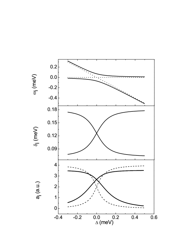
Figure 1: Peak energies, linewidths and intensity in function of detuning for the parameters of Ref. rei, : $\delta_{c}=0.09$ meV, $\delta_{x}=0.036$ meV, $V=0.075$ meV. The dashed line correspond to the maxima of $\rho_{11}(\omega)$.

In Fig. 2, we show the position of the peaks $\omega_{i}$ for a case in which $V$ was reduced to $V=0.022$ meV, so that there is no splitting of the energies for zero detuning.

Figure 2: Peak energies for the case of weak coupling. Parameters are $\delta_{c}=0.09$ meV, $\delta_{x}=0.036$ meV, $V=0.022$ meV.

IV.2 Position of the maxima

When $V\gg\delta_{c},\delta_{x}$, the spectral density $\rho_{11}(\omega)$ shows two maxima for all values of the detuning $\Delta$. The position of the maxima are given by some real roots of a polynomial of fifth degree obtained from the condition $\partial\rho_{11}(\omega)/\partial\omega=0$. As $V$ decreases, the two maxima merge into one for zero detuning, at a critical value $V_{c}$.

In Fig. 3 we represent $V_{c}$ as a function of one of the broadenings $\delta_{c}$ or $\delta_{x}$, keeping constant the other one. We can that as $\delta_{x}$ increases, $V_{c}$ also increases. However, the trend is the opposite as $\delta_{c}$ increases.

Figure 3: Critical coupling as a function of (a) linewidth of the cavity mode $\delta_{c}$, and (b) linewidth of exciton mode $\delta_{x}$

In Fig. 4 we plot the difference between the two maxima $\ \Delta E$ as function of $V$ for the case $\delta_{x}=\delta_{c}$. The experimentally measured Rabi splitting might be identified with $\ \Delta E$, but another possibility is to relate the Rabi splitting with $\omega_{2}-\omega_{1}=2x$ [see Eqs. (10)-(13)]. We believe that the latter approach is more physical if the experimental line can be fit by Eq. (10).

We can see from the figure that $\Delta E$ has a behavior of a square root as a function of $\Delta V=V-V_{c}$ for small $\Delta V$, while for large $V$, $\Delta E$ is proportional to $2V$, as expected.

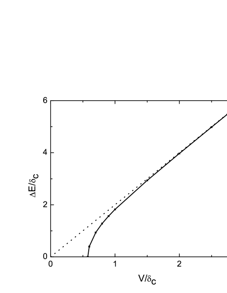
Figure 4: Separation between the maxima of $\rho_{11}(\omega)$ as a function of coupling contant $V$ for $\delta_{x}=\delta_{c}$ and $E_{x}=E_{c}$

IV.3 Spectral density for different detunings

The spectral density (assumed proportional to the photoluminiscence intensity) for different detuning $\Delta=E_{x}-E_{c}$, is presented in Fig. 5 for  parameters that correspond to  the particular experimental work of Reithmaier et al. rei in which the detuning was controlled by the tempertaure The anticrossing is clearly visible and the variation of the intensity profile is similar to the observed one. For negative detuning, the peak at lowest energy is more excitonic like and therefore has lower intensity than the other one, which has a greater admixture with the cavity mode. The situation is reversed for positive detuning.

Figure 5: Photoluminescense spectra for several values of detunning $\Delta=E_{x}-E_{c}$. The parameter used are the same as in Fig. 1 rei .

In Ref. reit, , the detuning was controlled by the application of a magnetic field. In Fig. 6 we show the corresponding theoretical curve, with the same qualitative trends as before. The coupling $V=0.046$ meV was adjusted in such a way that the difference between the maxima in $\rho_{11}(\omega)$ correspond to the reported Rabi splitting of $0.0956$ meV and half width at half maximum of the cavity and exciton modes $\delta_{c}=0.06$ meV and $\delta_{x}=0.01$ meV respectively (corresponding to half of the reported full width at half maximum).

Figure 6: (a) Photoluminescense spectra for several values of detuning, (b) Energy dispersion of the two emission modes. the uncoupled modes is indicated by dot lines. Parameters are $\delta_{c}=0.06$ meV, $\delta_{x}=0.01$ meV, $V=0.046$ meV

V Summary

We have studied a microscopic model that couples a cavity mode with an exciton, and includes coupling to two continua of bosonic excitations, which give rise to a homogeneous broadening of both modes. Although the model is not exactly solvable, we treat exactly the low-energy spectrum and provide expressions for the low-energy part of the spectral density of the cavity mode and the exciton. The former agrees with measured photoluminiscence spectra for several detunings.

Our approach provides a microscopic justification for simple phenomenological expressions for the position and widths of the two mixed modes, between the cavity mode and the exciton, when both modes have a homogeneous broadening.

References

- (1) J. P. Reithmaier, G. Seik, A. Loffler, C. Hofmann, S. Kuhn, S. Reitzenstein, L. V. Keldysh, V. D. Kulakovskii, T. L. Reinecke, and A. Forchel, Nature 432, 197 (2004).
- (2) T. Yoshie, A. Scherer, J. Hendrickson, G. Khitrova, H. M. Gibbs, G. Rupper, C. Ell, O. B. Shchekin and D. G. Deppe, Nature 432, 200 (2004).
- (3) D. Press, S. Gotzinger, S. Reitzenstein, C. Hofmann, A. Loffler, M. Kamp, A. Forchel and Y. Yamamoto, Phys. Rev. Lett. 98, 117402 (2007).
- (4) S. Reitzenstein, S. Munch, P. Franeck, A. Rahimi-Iman, A. Loffler, S. Hofling, L. Worschech, and A. Forchel, Phys. Rev. Lett. 103, 127401 (2009).
- (5) P. A. Dalgarno, M. Ediger, B. D. Gerardot, J. M. Smith, S. Seidl, M. Kroner, K. Karrai, P. M. Petroff, A. O. Govorov, and R. J. Warburton, Phys. Rev. Lett. 100, 176801 (2008).
- (6) L. M. León Hilario and A. A. Aligia, Phys. Rev. Lett. 103, 156802 (2009).
- (7) P.Michler, A. Kiraz, Becher, W. V. Schoenfeld, P. M. Petroff, Lidong Zhang, E. Hu, and A. Imamoglu, Science 290, 2282 (2000).
- (8) A. Imamoglu, D. D. Awschalom, G. Burkard, D. P. DiVincenzo, D. Loss, M. Sherwin, and A. Small, Phys. Rev. Lett 83, 4207 (1999).
- (9) C. J. Hood, M. S. Chapman, T. W. Lynn, H, J. Kimble, Phys. Rev. Lett. 80, 4157 (1998).
- (10) H. J. Carmichael, R. J. Brecha, M. G. Raizen and H. J. Kimble , Phys. Rev. A 40, 5516 (1989)
- (11) L. C. Andreani, G. Panzarini, and J-M Gérard, Phys. Rev. B 60, 13276 (1999)
- (12) L. M. León Hilario, A. Bruchhausen, A. M. Lobos, and A. A. Aligia, J. Phys.: Condens. Matter 19, 176210 (2007)
- (13) L. M. León Hilario, A. A. Aligia, A. M. Lobos, and A. Bruchhausen, Superlattices Microstruct. 43, 532 (2008)
- (14) A. Bruchhausen, L. M. León Hilario, A. A. Aligia, A. M. Lobos, A. Fainstein, B. Jusserand, R. André, Phys. Rev. B 78, 125326 (2008)