More Details on Analysis of Fractional-Order Lotka-Volterra Equation

Abstract

According to the long-memory principle appears in fractional-order dynamical systems, analysis of these systems is commonly more complicated than those described by nonlinear ordinary differential equations. Another difficulty is due to the fact that some classical tools such as the Lyapunov stability theorems cannot directly be applied to nonlinear fractional differential systems. The aim of this paper is to study the stability of a general form of the two-dimensional fractional-order Lotka-Volterra equation and numerically investigate the domain of attraction of its stable equilibrium points. It is also shown that the fractional-order Lotka-Volterra system can never have a stable focus although the linearized system has complex conjugate modes. Some other properties of the fractional-order Lotka-Volterra equation, which are not observed in integer-order case, are also discussed.

1 Introduction

The simplest model of predator-prey interactions was first developed independently by Alfred J. Lotka (Lotka, 1925) and Vito Volterra (Volterra, 1926). The classical two-dimensional Lotka-Volterra equation is given by:

$$\left\{\begin{array}[]{ll}\frac{dy_{1}}{dt}=ay_{1}-by_{1}y_{2},\\ \frac{dy_{2}}{dt}=-cy_{2}+by_{1}y_{2},\\ \end{array}\right.$$ (1)

where $y_{2}$ is the number of some predator (for example, wolves), $y_{1}$ is the number of its prey (for example, rabbits) and $a$, $b$, and $c$ are real parameters representing the interaction of the two species. This system and its extensions have been fully studied before by several researchers (Murray, 2003).

Recently, Ahmed et al. (2007) introduced the fractional-order Lotka-Volterra predator-prey system:

$$\left\{\begin{array}[]{ll}D^{\alpha}x_{1}(t)=x_{1}(t)(r-ax_{1}(t)-bx_{2}(t)),\\ D^{\alpha}x_{2}(t)=x_{2}(t)(-d+cx_{1}(t)),\\ \end{array}\right.$$ (2)

for some positive real constants $a,~{}b,~{}c,~{}d$, and $\alpha\in(0,1]$, and studied the stability of its equilibrium points (see Section 2 for the definition of fractional-order operators).

The aim of this paper is to study a more general form of the fractional-order Lotka-Volterra equation (as defined in (12)) in which the order of fractional derivatives are assumed to be different in general. Such a model may be used for better modelling and understanding the behavior of more complicated predator-pray systems.

Currently, nonlinear fractional-order systems constitute a challenging research area, mainly because some powerful classical tools such as the Lyapunov’s stability method cannot directly be applied to these systems. It is also a well-understood fact that determining the domain of attraction of stable equilibrium points of nonlinear fractional-order systems is not a straightforward task. The main reason for this difficulty is that the phase portrait of these systems cannot be plotted using the so-called isoclines. The long-memory principle of the fractional-order operators leads to some strange behaviors which are also discussed in this paper.

The rest of this paper is organized as follows. Some mathematical preliminaries are reviewed in Section 2. Stability of the fractional-order Lotka-Volterra equation under consideration is studied in Section 3. Section 4 discusses on the domain of attraction of the stable equilibrium points of the fractional-order Lotka-Volterra equation introduced in Section 3. Some properties of the fractional-order Lotka-Volterra equation are studied in Section 5, and finally Section 6 concludes the paper.

2 Mathematical background

2.1 fractional-order operators

Three kinds of definitions are widely used to define fractional-order derivatives: Grünwald-Letnikov derivative, Riemann-Liouville derivative and Caputo derivative (Podlubny, 1999). These three definitions are in general not equivalent. The definition of the fractional derivative given by Caputo has the advantage of only requiring initial conditions given in terms of integer-order derivatives. Clearly, such initial conditions represent well-understood features of a physical situation. In this paper, we will also use the Caputo derivative because of its applicability to real world models.

The Caputo fractional derivative of order $\alpha$ of function $f$, which is denoted by ${}_{a}^{C}D_{t}^{\alpha}f(t)$, is defined as

$$\small{{}_{a}^{C}D_{t}^{\alpha}f(t)=\left\{\begin{array}[]{ll}\frac{1}{\Gamma(n-\alpha)}\int_{a}^{t}\frac{f^{(n)}(x)}{(t-x)^{\alpha-n+1}}dx,~{}~{}~{}n-1<\alpha<n\\ f^{(n)}(t),\hskip 113.81102pt\alpha=n\\ \end{array},\right.}$$ (3)

where $t>a$ and $n\in\mathbb{Z}^{+}$. For simplicity of the notation, the symbol $D^{\alpha}$ is used in the rest of this paper to indicate ${}_{0}^{C}D_{t}^{\alpha}$.

2.2 stability of fractional-order systems

The following theorem will be instrumental in what follows.

Theorem 1

(Deng et al., 2007) Consider the $n$-dimensional linear fractional-order system:

$$\left\{\begin{array}[]{ll}D^{\alpha_{1}}x_{1}=a_{11}x_{1}+a_{12}x_{2}+\ldots+a_{1n}x_{n}\\ D^{\alpha_{2}}x_{1}=a_{21}x_{1}+a_{22}x_{2}+\ldots+a_{2n}x_{n}\\ \vdots\\ D^{\alpha_{n}}x_{n}=a_{n1}x_{1}+a_{n2}x_{2}+\ldots+a_{nn}x_{n}\\ \end{array},\right.$$ (4)

where all $\alpha_{i}$’s are rational numbers between $0$ and $1$. Assume $M$ be the lowest common multiple of the denominators $u_{i}$’s of $\alpha_{i}$’s, where $\alpha_{i}=v_{i}/u_{i}$, $(u_{i},v_{i})=1$, $u_{i},v_{i}\in\mathbb{Z}^{+}$, for $i=1,2,\ldots,n$. Define

$$\Delta(\lambda)=\left(\begin{array}[]{cccc}\lambda^{M\alpha_{1}}-a_{11}&-a_{12}&\ldots&-a_{1n}\\ -a_{21}&\lambda^{M\alpha_{2}}-a_{22}&\ldots&-a_{2n}\\ \vdots&\vdots&\ddots&\vdots\\ -a_{n1}&-a_{n2}&\ldots&\lambda^{M\alpha_{n}}-a_{nn}\\ \end{array}\right).$$ (5)

Then system (4) is globally asymptotically stable (in the Lyapunov sense) if all roots $\lambda$’s of the equation $\det(\Delta(\lambda))=0$ satisfy $|\arg(\lambda)|>\pi/(2M)$.

It is not difficult to show that the condition given in Theorem 1 is the necessary and sufficient condition for asymptotic stability of system (4) (see also (Matignon, 1996) for more details on this subject). Now, consider the nonlinear fractional-order system:

$$D^{\alpha_{i}}x_{i}(t)=f_{i}(x_{1},x_{2},\ldots,x_{n}),\quad i=1,2,\ldots,n,$$ (6)

where all $\alpha_{i}$’s are rational numbers between 0 and 1. Clearly, equilibrium points of (6) are roots of the equation

$$f_{i}(x_{1},x_{2},\ldots,x_{n})=0,\quad i=1,2,\ldots,n.$$ (7)

Now, let $\mathbf{x}^{*}=(x_{1}^{*},x_{2}^{*},\ldots,x_{n}^{*})$ be an equilibrium point of (6), i.e. $f_{i}(x_{1}^{*},x_{2}^{*},\ldots,x_{n}^{*})=0$ for $i=1,2,\ldots,n$. Suppose that $M$ is the lowest common multiple of the denominators $u_{i}$’s of $\alpha_{i}$’s, where $\alpha_{i}=v_{i}/u_{i}$, $(u_{i},v_{i})=1$, $u_{i},v_{i}\in\mathbb{Z}^{+}$, for $i=1,2,\ldots,n$. Then, according to Theorem 1 it can be easily shown that $\mathbf{x}^{*}$ is asymptotically stable if and only if the inequality:

$$|\arg(\lambda)|>\pi/2M,$$ (8)

holds for all roots $\lambda$’s of the equation:

$$\det\left({\rm diag}([\lambda^{M\alpha_{1}},\lambda^{M\alpha_{2}},\ldots,\lambda^{M\alpha_{n}}])-\mathbf{J}\right)=0,$$ (9)

where the notation ${\rm diag}([r_{1},r_{2},\ldots,r_{n}])$ denotes an $n\times n$ diagonal matrix as follows:

$${\rm diag}([r_{1},r_{2},\ldots,r_{n}])=\left(\begin{array}[]{cccc}r_{1}&0&\ldots&0\\ 0&r_{2}&\ldots&0\\ \vdots&\vdots&\ddots&\vdots\\ 0&0&\ldots&r_{n}\\ \end{array}\right),$$ (10)

and

$$\mathbf{J}=\partial\mathbf{f}/\partial\mathbf{x}|_{x^{*}},\quad\mathbf{f}=[f_{1}\quad f_{2}\quad\ldots\quad f_{n}]^{T}.$$ (11)

3 Stability analysis of the two-dimensional fractional-order Lotka-Volterra equation

In this paper, we mainly study the two-dimensional fractional-order Lotka-Volterra equation:

$$\left\{\begin{array}[]{ll}D^{\alpha}y_{1}=f_{1}(y_{1},y_{2})=y_{1}(a-by_{2}),\\ D^{\beta}y_{2}=f_{2}(y_{1},y_{2})=y_{2}(-c+by_{1}),\\ \end{array}\right.$$ (12)

where $\alpha$ and $\beta$ are positive rational constants. Note that it is not a considerable loss of generality to limit the studies to the case that both $\alpha$ and $\beta$ are rational numbers since, in practice, all numbers are stored with a limited precision in computer and moreover, one can find a rational number in any neighborhood of a given nonrational number. In the following, we discuss on the asymptotic stability of the equilibrium points of (12) in two cases separately.

3.1 Case 1: $\alpha$ and $\beta$ between 0 and 1

The stability theorem presented in Section 2.2 can directly be used to study the stability of the equilibrium points of (12) when both $\alpha$ and $\beta$ are rational numbers in the range $(0,1)$. In this case the system has two equilibrium points denoted as $\mathbf{Y}_{1}^{*}=(0,0)$ and $\mathbf{Y}_{2}^{*}=(c/b,a/b)$. The Jacobian matrices are calculated as

$$\mathbf{J}_{1}=\left(\begin{array}[]{cc}a&0\\ 0&-c\\ \end{array}\right),$$ (13)

and

$$\mathbf{J}_{2}=\left(\begin{array}[]{cc}0&-c\\ a&0\\ \end{array}\right),$$ (14)

respectively at $\mathbf{Y}_{1}^{*}$ and $\mathbf{Y}_{2}^{*}$. Assume that $\alpha=u/M$ and $\beta=v/M$ for some positive integers $u$, $v$, and $M$. At $\mathbf{Y}_{1}^{*}$, (9) concludes that

$$\det\left(\left(\begin{array}[]{cc}\lambda^{u}&0\\ 0&\lambda^{v}\\ \end{array}\right)-\left(\begin{array}[]{cc}a&0\\ 0&-c\\ \end{array}\right)\right)=\left(\lambda^{u}-a\right)\left(\lambda^{v}+c\right)=0.$$ (15)

So, the equilibrium point $\mathbf{Y}_{1}^{*}$ is stable if and only if all roots of (15) lie in the sector of stability defined by

$$|\arg(\lambda)|>\frac{\pi}{2M}.$$ (16)

But if $a>0$ or $c<0$ then at least one of the $u+v$ roots of (15) lie in the sector defined by $|\arg(\lambda)|<\pi/(2M)$ and consequently, the equilibrium point $\mathbf{Y}_{1}^{*}$ becomes unstable. Hence, the necessary condition for stability of $\mathbf{Y}_{1}^{*}$ is to have $a<0$ and $c>0$. Assuming $a<0$ and $c>0$, the roots of (15) are calculated as

$$\lambda=\sqrt[u]{|a|}e^{i(2h+1)\pi/u},\quad h=0,1,\ldots,u-1,$$ (17)

and

$$\lambda=\sqrt[v]{c}e^{i(2h+1)\pi/v},\quad h=0,1,\ldots,v-1,$$ (18)

where $i=\sqrt{-1}$. Clearly, all of the above roots lie in the sector of stability defined by (16) if and only if we have

$$\frac{\pi}{u}>\frac{\pi}{2M}\quad\mathrm{and}\quad\frac{\pi}{v}>\frac{\pi}{2M},$$ (19)

which concludes that

$$\alpha<2\quad\mathrm{and}\quad\beta<2,$$ (20)

considering the fact that $\alpha=u/M$ and $\beta=v/M$. As a result, $\mathbf{Y}_{1}^{*}$ is a stable equilibrium point of (12) if and only if we have $a<0$ and $c>0$ provided that $\alpha$ and $\beta$ are real numbers between 0 and 1. Note that the stability of $\mathbf{Y}_{1}^{*}$ is independent of the value assigned to $b$.

At $\mathbf{Y}_{2}^{*}$, (9) reads

$$\det\left(\left(\begin{array}[]{cc}\lambda^{u}&0\\ 0&\lambda^{v}\\ \end{array}\right)-\left(\begin{array}[]{cc}0&-c\\ a&0\\ \end{array}\right)\right)=\lambda^{u+v}+ac=0.$$ (21)

Clearly, if $a$ and $c$ satisfy the inequality $ac<0$ then (21) will have at least one root outside the region of stability defined by (16) and hence, $\mathbf{Y}_{2}^{*}$ will be unstable. So, the necessary condition for the stability of $\mathbf{Y}_{2}^{*}$ is that we have $ac>0$. Assuming $ac>0$, (21) yields

$$\lambda=\sqrt[u+v]{ac}e^{i(2h+1)\pi/(u+v)},\quad h=0,1,\ldots,u+v-1.$$ (22)

It can be easily shown that all of these roots lie in the sector of stability defined by (16) if and only if we have

$$\frac{\pi}{u+v}>\frac{\pi}{2M},$$ (23)

or equivalently,

$$\frac{u}{M}+\frac{v}{M}=\alpha+\beta<2.$$ (24)

But, inequality (24) is always satisfied since it is assumed that both $\alpha$ and $\beta$ are between 0 and 1. To sum up, $\mathbf{Y}_{2}^{*}$ is the stable equilibrium point of (12) if and only if we have $ac>0$ provided that $\alpha$ and $\beta$ are real numbers between 0 and 1. Note that the stability of $\mathbf{Y}_{2}^{*}$ is also independent of the value assigned to $b$. Figure 1 summarizes the stability properties of $\mathbf{Y}_{1}^{*}$ and $\mathbf{Y}_{2}^{*}$ in $a-c$ plane.

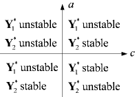
Figure 1: Stability properties of the equilibrium points of (12) in $a-c$ plane when both $\alpha$ and $\beta$ are rational numbers between 0 and 1.

3.2 Case 2: $\alpha$ and $\beta$ between 1 and 2

The stability theorem presented in Section 2.2 cannot directly be used to study the stability of the equilibrium points of (12) when $\alpha$ and/or $\beta$ are greater than unity. In order to study the stability of the equilibrium points of (12) when both $\alpha$ and $\beta$ are rational numbers between 1 and 2, first we should write this equation in an equivalent form such that the order of differentiation in all equations be between 0 and 1. Assuming $y_{3}=dy_{1}/dt$, $y_{4}=dy_{2}/dt$, $\alpha=1+\alpha_{1}$, and $\beta=1+\beta_{1}$, (12) can be written as

$$\left\{\begin{array}[]{ll}D^{\alpha_{1}}y_{3}=y_{1}(a-by_{2})=f_{1}(y_{1},y_{2},y_{3},y_{4}),\\ D^{\beta_{1}}y_{4}=y_{2}(-c+by_{1})=f_{2}(y_{1},y_{2},y_{3},y_{4}),\\ Dy_{1}=y_{3}=f_{3}(y_{1},y_{2},y_{3},y_{4}),\\ Dy_{2}=y_{4}=f_{4}(y_{1},y_{2},y_{3},y_{4}),\\ \end{array}\right.$$ (25)

where $\alpha_{1}=u/M$ and $\beta_{1}=v/M$ are rational numbers between 0 and 1. System (25) has two equilibrium points denoted as $\mathbf{Y}_{1}^{*}=(0,0,0,0)$ and $\mathbf{Y}_{2}^{*}=(c/b,a/b,0,0)$ (the state vector of the system is considered as $(y_{3},y_{4},y_{1},y_{2})$). The Jacobian matrices at $\mathbf{Y}_{1}^{*}$ and $\mathbf{Y}_{2}^{*}$ are obtained as

$$\mathbf{J}_{1}=\left(\begin{array}[]{cccc}a&0&0&0\\ 0&-c&0&0\\ 0&0&1&0\\ 0&0&0&1\\ \end{array}\right),$$ (26)

and

$$\mathbf{J}_{2}=\left(\begin{array}[]{cccc}0&-c&0&0\\ a&0&0&0\\ 0&0&1&0\\ 0&0&0&1\\ \end{array}\right),$$ (27)

respectively. At the first equilibrium point, (9) reads

$$\det\left(\left(\begin{array}[]{cccc}\lambda^{u}&0&0&0\\ 0&\lambda^{v}&0&0\\ 0&0&\lambda^{M}&0\\ 0&0&0&\lambda^{M}\\ \end{array}\right)-\left(\begin{array}[]{cccc}a&0&0&0\\ 0&-c&0&0\\ 0&0&1&0\\ 0&0&0&1\\ \end{array}\right)\right)\\ =\left(\lambda^{u}-a\right)\left(\lambda^{v}+c\right)\left(\lambda^{M}-1\right)^{2}=0.$$ (28)

Equation (28) always has two roots at $\lambda=1$, which do not lie in the sector of stability defined by (16). Therefore, $\mathbf{Y}_{1}^{*}$ is an unstable equilibrium point for (12) for all values of $\alpha$ and $\beta$ between 1 and 2 regardless of the values assigned to $a$, $b$, and $c$.

At the second equilibrium point, (9) concludes that

$$\det\left(\left(\begin{array}[]{cccc}\lambda^{u}&0&0&0\\ 0&\lambda^{v}&0&0\\ 0&0&\lambda^{M}&0\\ 0&0&0&\lambda^{M}\\ \end{array}\right)-\left(\begin{array}[]{cccc}0&-c&0&0\\ a&0&0&0\\ 0&0&1&0\\ 0&0&0&1\\ \end{array}\right)\right)\\ =\left(\lambda^{u+v}+ac\right)\left(\lambda^{M}-1\right)^{2}=0,$$ (29)

which also has two roots at $\lambda=1$, outside the sector of stability. Hence, $\mathbf{Y}_{2}^{*}$ is also an unstable equilibrium point for (12) for all values of $\alpha$ and $\beta$ between 1 and 2 regardless of the special values assigned to $a$, $b$, and $c$.

4 Domain of attraction of stable equilibrium points

In the previous section we proved that the equilibrium points of (12) are unstable for all values of $\alpha$ and $\beta$ between 1 and 2. In the following, we discuss on the domain of attraction of the stable equilibrium points of (12) when both $\alpha$ and $\beta$ are between 0 and 1. According to the lack of analytical tools, most of the discussions in this section are based on numerical calculations.

4.1 Domain of attraction of $\mathbf{Y}_{1}^{*}=(0,0)$

According to Fig. 1, $\mathbf{Y}_{1}^{*}$ is a stable equilibrium point for (12) (and consequently, has a domain of attraction) if and only if we have $a<0$ and $c>0$, provided that both $\alpha$ and $\beta$ are rational numbers between 0 and 1. Figure 2 shows the equilibrium points of (12) and the corresponding isoclines in 9 different regions of the $y_{1}$-$y_{2}$ plane assuming $a=b=-c=-1$ (clearly, the following discussions can be extended to other values of $a,~{}b,$ and $c$ provided that $a<0$ and $c>0$). In the following, first we study the domain of attraction of $\mathbf{Y}_{1}^{*}$ assuming $\alpha=\beta=1$ and then extend the results to the case where both $\alpha$ and $\beta$ are between 0 and 1. Note that in the latter case the isoclines cannot directly be used to determine the domain of attraction.

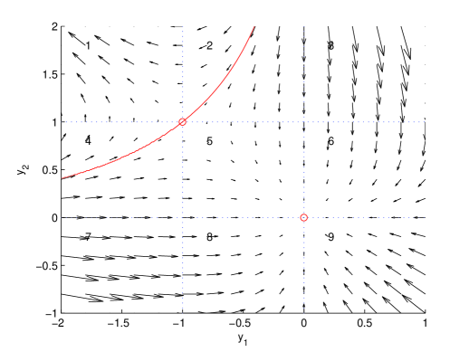
Figure 2: Isoclines of (12) assuming $\alpha=\beta=-a=-b=c=1$. The solid curve is the border of the domain of attraction of $\mathbf{Y}_{1}^{*}$.

First, assume that $\alpha=\beta=1$. In this case, according to the isoclines shown in Fig. 2, if $y_{1}(0)$ and $y_{2}(0)$ lie in one of the regions 3, 5, 6, 7, 8, and 9 of Fig. 2 then the state trajectories of (12) move toward the origin by increasing the time. But, if the initial conditions lie in region 1 then the state trajectories move toward infinity. It is also clear that some parts of regions 2 and 4 in Fig. 2 belong to the domain of attraction of $\mathbf{Y}_{1}^{*}$. The border of the domain of attraction in regions 2 and 4 can be determined by solving the following initial value problem:

$$\frac{dy_{2}}{dy_{1}}=\frac{f_{2}}{f_{1}}=\frac{y_{2}(by_{1}-c)}{y_{1}(a-by_{2})},\quad y_{2}\left(\frac{c}{b}\right)=\frac{a}{b},$$ (30)

the solution of which is implicitly given by

$$y_{2}^{a}y_{1}^{c}=\left(\frac{a}{b}\right)^{a}\left(\frac{c}{b}\right)^{c}e^{b(y_{1}+y_{2})-(a+c)}.$$ (31)

The solid curve in Fig. 2 shows the solution of the above equation. To sum up, all points in the right-hand side of this curve belong to the domain of attraction of $\mathbf{Y}_{1}^{*}$ when $\alpha=\beta=1$. Note that regions 1, 5, 6, and 9 in Fig. 2 have the property that all of the state trajectories that begin from any point inside them will remain in these regions forever.

In fractional case, however, according to the long memory principle the border of the domain of attraction cannot be determined analytically. The dash-dotted and solid curves in Fig. 3 show the border of the domain of attraction when $\alpha=\beta=0.1$ and $\alpha=\beta=1$, respectively assuming $a=b=-c=-1$. In this figure, the dash-dotted curve has been obtained by using numerical techniques (all simulations of this paper are performed based on the numerical method proposed in (Diethelm et al., 2002), which can be used to find the solution of a Caputo definition based fractional differential equation). Clearly, all points in the right-hand side of this curve belong to the domain of attraction. As it can be observed, the domain of attraction of $\mathbf{Y}_{1}^{*}$ becomes smaller by decreasing $\alpha$ and $\beta$. Numerical simulations also show that the border of the domain of attraction for the values of $\alpha$ and $\beta$ between 0 and 0.1 is almost the same as the dash-dotted curve in Fig. 3. In general, precise simulations confirm the fact that regions 3, 5, 6, 7, 8, and 9 in Fig. 3 belong to the domain of attraction of $\mathbf{Y}_{1}^{*}$ for all values of $\alpha$ and $\beta$ between 0 and 1. Moreover, all state trajectories that begin from any point in regions 5, 6, 8, and 9 have the property that remain inside these regions forever.

Figure 3: The solid curve: the border of the domain of attraction of $\mathbf{Y}_{1}^{*}$ when $\alpha=\beta=1$; the dash-dotted curve: the border of the domain of attraction of $\mathbf{Y}_{1}^{*}$ when $\alpha=\beta=0.1$.

4.2 Domain of attraction of $\mathbf{Y}_{2}^{*}=(c/b,a/b)$

According to Fig. 1, $\mathbf{Y}_{2}^{*}$ is a stable equilibrium point for (12) (and consequently, has a domain of attraction) if and only if we have $a,c<0$ or $a,c>0$, provided that both $\alpha$ and $\beta$ are rational numbers between 0 and 1. Figure 4 shows the equilibrium points of (12) and the corresponding isoclines in 9 different regions of the $y_{1}$-$y_{2}$ plane assuming $a=b=-c=-1$. According to this figure, the third quadrant of the $y_{1}$-$y_{2}$ plane is exactly equal to the domain of attraction of $\mathbf{Y}_{2}^{*}$ when $\alpha=\beta=1$.

Similarly, precise numerical simulations show that the first (third) quadrant of the $y_{1}$-$y_{2}$ plane is exactly equal to the domain of attraction of $\mathbf{Y}_{2}^{*}$ when $b>0$ ($b<0$) assuming that $a,c>0$ and $\alpha,\beta\in(0,1]$. It is also observed that for all values of $a,c<0$ and $\alpha,\beta\in(0,1]$ the first (third) quadrant of the $y_{1}$-$y_{2}$ plane is exactly equal to the domain of attraction of $\mathbf{Y}_{2}^{*}$ when $b<0$ ($b>0$).

Note that when $a$ and $c$ are chosen such that $\mathbf{Y}_{2}^{*}$ is a stable equilibrium point, it seems that it is a stable focus for all values of $\alpha,\beta\in(0,1]$, but it will be shown in the next section that this statement is not true.

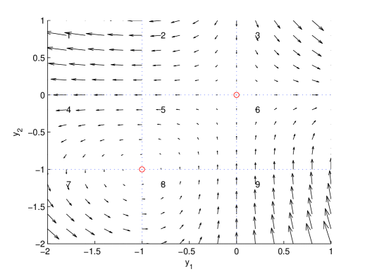
Figure 4: Isoclines of (12) assuming $\alpha=\beta=a=-b=c=1$.

5 Some properties of the fractional-order Lotka-Volterra equation

In this section, we numerically investigate some properties of the two-dimensional fractional-order Lotka-Volterra equation assuming $0<\alpha<1$ and $0<\beta<1$.

Figure 5 shows the phase-plane portrait of (12) for $0\leq t\leq 80$ assuming $\alpha=0.9$, $\beta=0.8$, $a=c=-b=1$, and $y_{1}(0)=y_{2}(0)=-0.5$ . For these values of parameters, the system has a stable equilibrium point at $(-1,-1)$ and the third quadrant of the $y_{1}$-$y_{2}$ plane is exactly equal to the domain of attraction of this equilibrium point. As it is expected, the state trajectory of the system moves toward this stable equilibrium point, which seems to be a stable focus. Figure 6 shows the region around this stable equilibrium point with more details. As it is observed, the state trajectory of the system does not behave as it does near a stable focus. Considerable number of simulations confirm the fact that $\textbf{Y}_{2}^{*}$ (as well as $\textbf{Y}_{1}^{*}$) can never act as a stable focus. As another fact, the state trajectory of the fractional-order Lotka-Volterra system may intersect itself.

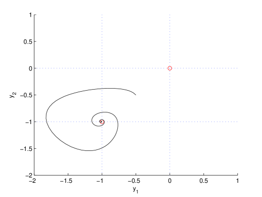
Figure 5: The phase-plane portrait of (12) when $\alpha=0.9$, $\beta=0.8$, $a=c=-b=1$ and $y_{1}(0)=y_{2}(0)=-0.5$ for $0\leq t\leq 80$.

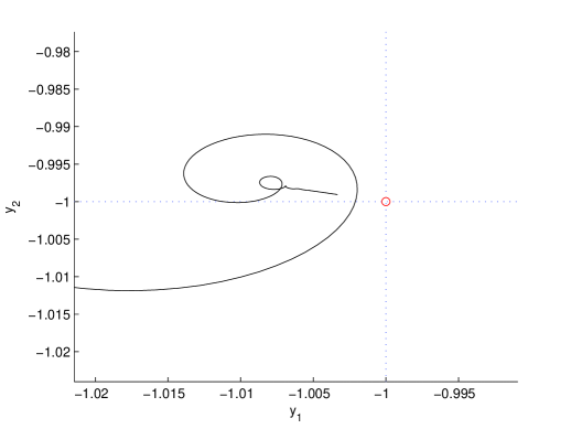
Figure 6: Figure 5 focused around $(-1,-1)$.

Note that inequality $D^{\alpha}y(t_{0})>0,~{}(0<\alpha<1)$ does not conclude that $y^{\prime}(t_{0})>0$, i.e. we may have $D^{\alpha}y(t_{0})>0$ while $y$ is not increasing at $t=t_{0}$. That is why in the region defined by $-2<y_{2}<-1$ and $-2<y_{1}<-1$ in Fig. 5, $f_{2}$ is positive while $y_{2}$ is not a uniformly increasing function of time.

Another observation is that the qualitative behavior of the state trajectories of (12), in general, depend on the initial conditions of the system. For example, consider (12) with $\alpha=0.2$, $\beta=0.9$, and $a=c=-b=1$ subject to the initial conditions $y_{1}(0)=-0.01$ and $y_{2}(0)=-0.99$. The phase portrait of this system is shown in Fig. 7 for $0\leq t\leq 80$. As it is observed, the state trajectory of system intersects itself and creates a tie. Figure 8 shows the phase portrait of the same system assuming the initial conditions $y_{1}(0)=-0.1$ and $y_{2}(0)=-0.99$. In this figure, the tie has been removed. This property is a direct consequence of the long memory principle which exists only in fractional-order systems.

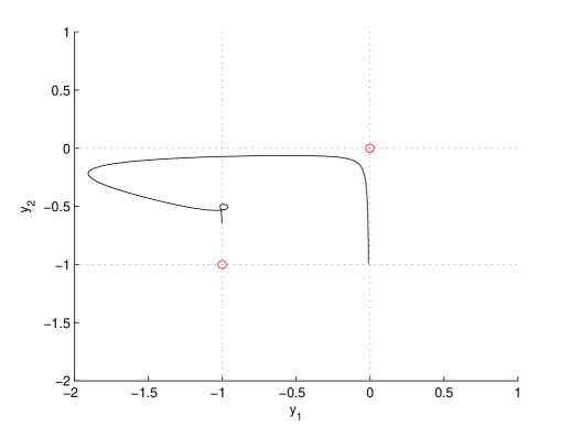
Figure 7: The phase-plane portrait of (12) when $\alpha=0.2$, $\beta=0.9$, $a=c=-b=1$, $y_{1}(0)=-0.01$ and $y_{2}(0)=-0.99$.

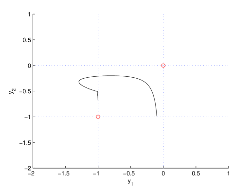
Figure 8: The phase-plane portrait of (12) when $\alpha=0.2$, $\beta=0.9$, $a=c=-b=1$, $y_{1}(0)=-0.1$ and $y_{2}(0)=-0.99$.

Note that unlike the integer-order Lotka-Volterra equation which exhibits stable limit cycles, the state trajectories of (12) can never produce a limit cycle for the values of $\alpha$ and $\beta$ between 0 and 1.

6 Discussion and conclusion

In this paper, we studied a general form of the two-dimensional fractional-order Lotka-Volterra equation. Stability of the equilibrium points was discussed and the domain of attraction of stable equilibrium points was determined in several cases. It was also numerically shown that the stable equilibrium points of this system can never act as a stable focus. As another fact, it was observed that the qualitative behavior of the state trajectories of this system depend on the initial conditions. Specially, we observed that for certain values of the parameters and initial conditions the phase portrait of this system can intersect itself and produce one or more ties.

Some other questions still remain unanswered. It is a well-known fact that for a system described by

$$\dot{\mathbf{x}}=\mathbf{f}(\mathbf{x},t),$$ (32)

where $\mathbf{x}\in\mathbb{R}^{n}$ is the state vector of system, the type of the equilibrium point $\mathbf{x}=\mathbf{x}^{*}$ can be investigated by examining the eigenvalues of the Jacobian matrix $\mathbf{J}=\partial\mathbf{f}/\partial\mathbf{x}|_{\mathbf{x}=\mathbf{x}^{*}}$ (Slotine and Li, 1991). It concludes that $\mathbf{x}=\mathbf{x}^{*}$ is either a stable (unstable) node or a stable (unstable) focus or a saddle point. Note that in this case the eigenvalues of the Jacobian matrix are actually the modes of the linearized system. But, the discussions of this paper showed that according to the long memory principle, the type of the equilibrium points of a fractional-order system cannot be determined by investigating the eigenvalues of the corresponding Jacobian matrix. More precisely, linearizing (12) around any of its equilibrium points leads to

$$\left(\begin{array}[]{c}D^{\alpha}Y_{1}\\ D^{\beta}Y_{2}\\ \end{array}\right)=\left(\begin{array}[]{cc}a&-by_{1}^{2}\\ by_{2}^{2}&-c\\ \end{array}\right)^{*}\left(\begin{array}[]{c}Y_{1}\\ Y_{2}\\ \end{array}\right),$$ (33)

where $Y_{1}=y_{1}-y_{1}^{*}$ and $Y_{2}=y_{2}-y_{2}^{*}$. By taking the Laplace transform from both sides of the above equation, the characteristic equation of the linearized system is obtained as

$$\left|\begin{array}[]{cc}s^{\alpha}-a&b(y_{1}^{*})^{2}\\ -b(y_{2}^{*})^{2}&s^{\beta}+c\\ \end{array}\right|=0,$$ (34)

where $s$ stands for the Laplace variable. The roots of the above equation are modes of the linearized system (33), which are distributed on a Riemann surface with infinity number of Riemann sheets (clearly, if both $\alpha$ and $\beta$ be rational numbers then the corresponding Riemann surface will have a finite number of Riemann sheets). In fact, the discussions of this paper showed that, unlike the classical case, in dealing with fractional-order systems the modes of the linearized system cannot be used the determine the type of the equilibrium points of system. The relation between the modes of the linearized fractional-order system and the type of its equilibrium points remains as a challenging question.

References

- Lotka (1925) A.J. Lotka. Elements of Physical Biology. Baltimore, Williams & Wilkins Co., 1925.
- Volterra (1926) V. Volterra. Variazioni e fluttuazioni del numero d’individui in specie animali conviventi. Mem. R. Accad. Naz. dei Lincei. 2(VI), 1926.
- Murray (2003) J.D. Murray. Mathematical Biology I: An Introduction. Springer-Verlag, 2003.
- Ahmed et al. (2007) E. Ahmed, A.M.A. El-Sayed, and H.A.A. El-Saka. Equilibrium points, stability and numerical solutions of fractional-order predator-prey and rabies models. ” J. Math. Anal. Appl., 325: 542-553, 2007.
- Podlubny (1999) I. Podlubny. Fractional Differential Equations. Academic Press, 1999.
- Deng et al. (2007) W. Deng, C. Li, and J. Lü. Stability analysis of linear fractional differential system with multiple time delays. Nonlinear Dyn., 48: 409-416, 2007.
- Matignon (1996) D. Matignon. Stability result on fractional differential equations with applications to control processing. In: Proceedings of IMACS-SMC, pp. 963-968, Lille, France, 1996.
- Diethelm et al. (2002) K. Diethelm, N.J. Ford, and A.D. Freed. A predictor-corrector approach for the numerical solution of fractional differential equations. Nonlinear Dyn., 29: 3-22, 2002.
- Slotine and Li (1991) J.E. Slotine and W. Li. Applied nonlinear control. Prentice Hall, Englewood Cliffs, N.J., 1991.