Improving forecasting performance using covariate-dependent copula models

Abstract

Copulas provide an attractive approach for constructing multivariate distributions with flexible marginal distributions and different forms of dependences. Of particular importance in many areas is the possibility of explicitly forecasting the tail-dependences. Most of the available approaches are only able to estimate tail-dependences and correlations via nuisance parameters, but can neither be used for interpretation, nor for forecasting. Aiming to improve copula forecasting performance, we propose a general Bayesian approach for modeling and forecasting tail-dependences and correlations as explicit functions of covariates. The proposed covariate-dependent copula model also allows for Bayesian variable selection among covariates from the marginal models as well as the copula density. The copulas we study include Joe-Clayton copula, Clayton copula, Gumbel copula and Student’s t-copula. Posterior inference is carried out using an efficient MCMC simulation method. Our approach is applied to both simulated data and the S&P 100 and S&P 600 stock indices. The forecasting performance of the proposed approach is compared with other modeling strategies based on log predictive scores. Value-at-Risk evaluation is also preformed for model comparisons.

1 Introduction

Copula modeling is an active research area dating back to Sklar’s Theorem [40]. The theorem states that any multivariate cumulative distribution function can be written in terms of univariate marginal distributions and a copula function. Allowing the researchers to specify the marginal distributions separately from the copula function that links theses distributions to form the joint distribution, copula models provide a great deal of flexibility in modeling multivariate distributions, and thus become very popular in multivariate analysis. The related studies include, but are not limited to, an introduction to copulas [29], research on dependences and extreme value distributions with copulas [19], research on the construction of multivariate dependences using bivariate copulas [23], and approaches in copula estimation (see Jaworski et al. [17] for a review) including pair-copula constructions (see Czado [4] and references therein).

Copula models have been widely used in forecasting as well as in risk evaluation due to their capacity to model tail-dependences and correlations (see Patton [33] and Smith [42] for recent surveys). Dobrić and Schmid [6] use nonparametric methods to estimate the lower tail-dependence in bivariate copulas with continuous marginals for assets in German DAX30 stock index. Schmidt and Stadtmuller [37] explore the tail-dependence estimators for the tail copula with exchange rates for Deutsche Mark to US dollars, and Japanese Yen to US dollars. Draisma et al. [7] use hypothesis testing to detect the dependence of extreme events when they are asymptotically independent. A case study for rain-wind data of modeling the asymptotic dependence can be found in Ledford and Tawn [24]. Tail dependences result in the tail risk of value-at-risk (VaR). One of the main difficulties in forecasting VaR of portfolio is to model the tail-dependence structure and forecast the future tail-dependence. Extensive empirical studies (e.g., Huang et al. [16], Siburg et al. [39]) show that a copula model with accurately specified tail-dependence structure, especially in the lower tail-dependence, yields better VaR forecasting.

In copula-based tail-dependence forecasting, letting the tail-dependences and the Kendall’s $\tau$ in copula modeling be fixed numbers is very restrictive. This is particularly true in financial time-series applications, where the tail-dependences have been shown to vary with time [e.g., 32] and be affected by volatility information [e.g., 35]. Therefore, it is natural to condition on the available information, and thus we are led to study the conditional structure in tail-dependences. Despite the vast literature in tail-dependence estimation, little attempts have been made to investigate the factors that affect the variation of tail-dependences, not to mention using these factors to model tail-dependences and improve forecasting performance. This is partially because the computational complexity is still a challenge in many situations. Moreover, most approaches for modeling rank correlations and tail-dependences using existing copulas require firstly modeling intermediate parameters and thereafter obtaining them, which is inconvenient to link the correlations and tail-dependences directly with available covariates.

In this paper, we use feature to describe a characteristic in the univariate and multivariate densities (e.g. Kendall’s $\tau$ and tail-dependence are two features of a copula, while mean, variance, skewness and kurtosis are features of a univariate density). We propose a general Bayesian approach for copula modeling and forecasting with explanatory variables introduced in both tail-dependences and Kendall’s $\tau$ of the copula function. This construction allows us to explore the drivers of different forms of dependences, and obtain more informative forecasting based on available information. Variable selection is carried out in the features of marginal models as well as the copula features. We propose an efficient Markov chain Monte Carlo (MCMC) simulation method for posterior inference which is also used to calculate the predictive densities based on posterior draws.

The outline of the paper is as follows. Section 2 introduces the covariate-dependent copula model. We discuss the prior specification for the model and present the general form of the inferential approach in Section 3. Section 4 presents the details of the MCMC scheme. In Section 5, we demonstrate the advantages of including covariates in the dependences by evaluating the out-of-sample forecasting performances on simulated data. In Section 6, we use our proposed model to forecast the daily returns on the S&P 100 and S&P 600 stock market indices and make comparisons with other competing modeling strategies. Section 7 concludes the paper and discusses some potential directions for further research. The appendix documents the computational details used in the MCMC scheme.

2 The covariate-dependent copula model

A copula is a multivariate distribution that separates the univariate marginal distributions and the multivariate dependence structure. The correspondence between a multivariate distribution $F(x_{1},...,x_{M})$ and a copula function $C(u_{1},...,u_{M})$ can be expressed as

$$F(x_{1},...,x_{M})=F(F_{1}^{-1}(u_{1}),...,F_{M}^{-1}(u_{M}))=C(u_{1},...,u_{M})=C(F_{1}(x_{1}),...,F_{M}(x_{M})),$$

where the correspondence is one-to-one with continuous marginal distributions. Copulas provide a general approach for constructing flexible multivariate densities [19]. For example, the bivariate Gaussian copula $C(u_{1},u_{2}|\rho)=\Psi(F_{1}^{-1}(u_{1}),F_{2}^{-1}(u_{2})|\rho)$, with the correlation $\rho$, is a relaxed Gaussian density in the sense that $F_{1}(\cdot)$ and $F_{2}(\cdot)$ do not need to be normal [34].

2.1 Dependence concepts

Modeling the multivariate dependence typically involves quantifying two important quantities: tail-dependence and correlation. A key feature in copula models is that the multivariate dependence does not depend on marginal densities.

In copula models, the tail-dependence describes the concordance between extreme values of random variables $X_{1}$ and $X_{2}$. The lower tail-dependence $\lambda_{L}$ and the upper tail-dependence $\lambda_{U}$ can be expressed in terms of bivariate copulas:

$$\lambda_{L}= \lim_{u\to 0^{+}}p(X_{1}<F_{1}^{-1}(u)|X_{2}<F_{2}^{-1}(u))=\lim_{u\to 0^{+}}\frac{C(u,u)}{u},$$

$$\lambda_{U}= \lim_{u\to 1^{-}}p(X_{1}>F_{1}^{-1}(u)|X_{2}>F_{2}^{-1}(u))=\lim_{u\to 1^{-}}\frac{1-2u+C(u,u)}{1-u}.$$

Not all copulas have both lower and upper tail-dependences. For single-parameter copulas, which is only able to capture one side of the tail dependences, like the Clayton and the Gumbel copula, a simple way to achieve the same effect is to rotate the copula by 180 degrees.

The correlation between two variables is usually measured with rank correlations such as Kendall’s $\tau$:

$$\tau=4\int\int F(x_{1},x_{2})\mathrm{d}F(x_{1},x_{2})-1=4\int\int C(u_{1},u_{2})\mathrm{d}C(u_{1},u_{2})-1.$$

An attractive property of Kendall’s $\tau$ is that it is invariant with respect to strictly monotonic transforms. In this paper, we focus on modeling the correlation in terms of Kendall’s $\tau$. Other types of correlations, like Spearman’s rank correlation, can be equally well modeled with our method. For measuring the dependences in trivariate distributions, one may consider using a three-dimensional version of correlations [11]. Correlations in higher dimensions are usually estimated pairwisely.

2.2 The reparameterized copula

In this section, we describe how to reparameterize the copula function so that the parameters highlight the copula features of interest. The default parameters in most copula functions do not directly represent the copula features, such as the tail-dependences and Kendall’s $\tau$. We demonstrate the parameterization with the widely used two-parameter Joe-Clayton copula, which is flexible to be reparameterized in terms of any pairwise combination of lower tail-dependence, upper tail-dependece, and Kendal’s $\tau$.

Our copula modeling approach is general and can be applied to model any copulas. In Section 6, as well as our computer program, we extend our model class to Clayton copula, Gumbel copula, and Student’s t-copula. The popular vine copula construction [1, 5] can also be used to extend our bivariate copula modeling to higher dimensions with discrete and continuous margins, but requires further extensive work and will be discussed in a separate paper.

2.2.1 The Joe-Clayton copula

The Joe-Clayton copula function (also known as the BB7 copula), introduced by Joe [19], can be written as

$$C(u,v|\theta,\delta)= \eta(\eta^{-1}(u)+\eta^{-1}(v))$$

$$= 1-\left[1-\left\{\left(1-\bar{u}^{\theta}\right)^{-\delta}+\left(1-\bar{v}^{\theta}\right)^{-\delta}-1\right\}^{-1/\delta}\right]^{1/\theta},$$

where $\eta(s)=1-[1-(1+s)^{-1/\delta}]^{1/\theta}$, $\theta\geq 1$, $\delta>0$, $\bar{u}=1-u$, and $\bar{v}=1-v$. The copula density function for the Joe-Clayton copula is

$$\begin{split}c(u,v|\theta,\delta)=\frac{\partial^{2}C(u,v,\theta,\delta)}{\partial u\partial v}=&\left[T_{1}(u)T_{1}(v)\right]^{-1-\delta}T_{2}(u)T_{2}(v)L_{1}^{-2(1+\delta)/\delta}\\ &\times(1-L_{1}^{-1/\delta})^{1/\theta-2}\left[(1+\delta)\theta L_{1}^{1/\delta}-\theta\delta-1\right],\end{split}$$ (1)

where $T_{1}(s)=1-(1-s)^{\theta}$, $T_{2}(s)=(1-s)^{\theta-1}$ and $L_{1}=T_{1}(v)^{-\delta}+T_{1}(u)^{-\delta}-1$.

The lower and upper tail-dependences for Joe-Clayton copula are $\lambda_{L}=2^{-1/\delta}$ and $\lambda_{U}=2-2^{1/\theta}$, respectively. Previous work for Joe-Clayton copula includes the time-varying dependence modeling with symmetric version of the Joe-Clayton copula [32] and the development of multivariate dependence modeling via a vine structure based on bivariate copulas such as the Joe-Clayton copula [e.g., 1, 5].

The Kendall’s $\tau$ of the Joe-Clayton copula for the case $1\leq\theta<2$ can be found in Smith and Khaled [41], where only moderate level of correlation is possible. We extend it to $\theta\geq 2$ and present the full expression for all $\theta\geq 1$:

$$\tau(\theta,\delta)=\begin{cases}1-2/[\delta(2-\theta)]+4B\left(\delta+2,2/\theta-1\right)/(\theta^{2}\delta)&1\leq\theta<2;\\ 1-\left[\psi(2+\delta)-\psi(1)-1\right]/\delta&\theta=2;\\ 1-2/[\delta(2-\theta)]-4\pi/\left[\theta^{2}\delta(2+\delta)\sin(2\pi/\theta)B\left(1+\delta+2/\theta,2-2/\theta\right)\right]&\theta>2,\end{cases}$$

where $B(\cdot)$ is the beta function and $\psi(\cdot)$ is the digamma function. By the dominated convergence theorem, Kendall’s $\tau$ is continuous for all $\theta\geq 1$. If we employ the equations $\delta=-\log 2/\log\lambda_{L}$ and $\theta=\log 2/\log(2-\lambda_{U})$ from the previous results, we can rewrite Kendall’s $\tau$ in terms of lower and upper tail-dependences as $\tau(\lambda_{L},\lambda_{U})$. See Figure 1 for a contour plot of these relationships.

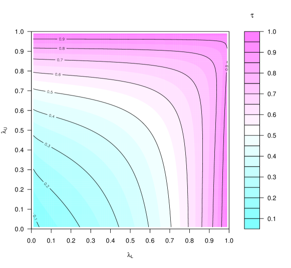
Figure 1: The contour plot of the Kendall’s $\tau$ with respect to lower tail-dependence ($\lambda_{L}$) and upper tail-dependence ($\lambda_{U}$) for the Joe-Clayton copula.

2.2.2 Reparametrization

To simplify the interpretation of the features in a copula model, we parameterize it in terms of the lower tail-dependence $\lambda_{L}$ and Kendall’s $\tau$,

$$C(u,v|\lambda_{L},\tau)= 1-\left[1-\left\{\left[1-\bar{u}^{\log 2/{\log(2-\tau^{-1}(\lambda_{L}))}}\right]^{\log 2/{\log\lambda_{L}}}\right.\right.$$

$$\hskip 51.21504pt\left.\left.+\left[1-\bar{v}^{\log 2/{\log(2-\tau^{-1}(\lambda_{L}))}}\right]^{\log 2/{\log\lambda_{L}}}-1\right\}^{\log\lambda_{L}/\log 2}\right]^{{\log(2-\tau^{-1}(\lambda_{L}))}/\log 2},$$

where $\tau^{-1}(\lambda_{L})=\lambda_{U}=2-2^{1/\theta}$ is the inverse function of Kendall’s $\tau$ given $\lambda_{L}$. The related reparametrized copula density is obtained by substituting $\delta=-\log 2/\log\lambda_{L}$ and $\theta=\log 2/\log(2-\tau^{-1}(\lambda_{L}))$ in Equation (1).

There are also alternative reparametrization schemes that allow for modeling lower and upper tail dependences $(\lambda_{L},\lambda_{U})$, or upper tail dependence and Kendall’s $\tau$ $(\lambda_{U},\tau)$, as shown in our simulation study and real data application. In principle, there is no difference among using parameterization in terms of $(\lambda_{L},\tau)$, $(\lambda_{L},\lambda_{U})$ and $(\lambda_{U},\tau)$ with regard to the Joe-Clayton copula if we are only interested in modeling the features as constants. When any two of the three parameterizations are used, the third can be easily derived due to the deterministic relationships among lower tail-dependence, upper tail-dependence and Kendall’s $\tau$, as shown in Figure 1.

Our parameterization has two primary advantages. Firstly, it makes it easier to specify the prior information in the Bayesian approach highlighted in Section 3. Secondly, and more importantly, the parameterization makes it possible to directly link correlations and tail-dependences to covariates, which yields conditional forecasting of the dependences. See Section 2.3 for the details.

2.3 Covariate-dependent copula features

We now introduce a covariate-dependent copula model that allows the copula features to be linked to the observed covariates. A prominent example is the covariate-dependent correlation and tail-dependences in a bivariate copula:

$$\tau=l_{\tau}^{-1}(\bm{X}\bm{\beta}_{\tau}),~{}\mathrm{and}~{}\lambda=l_{\lambda}^{-1}(\bm{X}\bm{\beta}_{\lambda}),$$ (2)

where $\lambda$ without subscripts represents the dependences in the lower and/or upper tails; $\tau$ is Kendall’s $\tau$; $\bm{X}$ is the set of covariates matrix used in the two margins and $\bm{\beta}$ with subscripts is the corresponding coefficients vector. Furthermore, $l_{\tau}(\cdot)$ and $l_{\lambda}(\cdot)$ are suitable link functions that connect $\lambda$ and $\tau$ with $\bm{X}$.

This covariate-dependent parameterization has three primary advantages. First, our approach makes it possible to use all marginal information to model the tail-dependences, which also yields the conditional forecasting on tail-dependences. Second, this parameterization can be applied to a rich class of copulas. Besides, ARMA-like variation in tail-dependences [32] and GARCH-like dependences in the dependences [26] can be considered as special cases of our model since their lagged dependences and volatility variables can be used as the covariates in our model. Third, it is straightforward to construct the likelihood function in our model (See Section 4 for the MCMC details) and variable selection can be used to select meaningful covariates that influence the dependences and also prevent overfitting.

Compared with the bivariate DCC-GARCH model [10] and the bivariate volatility model [47], our approach not only leads to a more insightful interpretation of the features, but allows for conditional heteroscedasticity in the dependences and generates more accurate forecasts as a result. See a detailed simulation study in Section 5.3 and real data forecasting analysis in Section 6.3.

2.4 Marginal models

In this paper we use margins as a synonym for marginal models. In principle, the copula approach can be used with any margins, but we assume the margins to be split-t distributions [25] in our simulation studies in Section 5 and the real data application in Section 6. The split-t is a flexible four-parameter distribution with the Student’s t distribution, the asymmetric normal and the symmetric normal distributions as its special cases. See Li et al. [25] for its properties.

Following Li et al. [25], we allow the mean $\bm{\mu}_{k}$, the scale $\bm{\phi}_{k}$, the degrees of freedom $\bm{\nu}_{k}$ and the skewness $\bm{\kappa}_{k}$ of the split-$t$ density in the k:th margins to be linked to covariates in the following matrix form:

$$\bm{\mu}_{k}=\bm{X}_{k}\bm{\beta}_{\mu_{k}},~{}\bm{\nu}_{k}=\exp(\bm{X}_{k}\bm{\beta}_{\nu_{k}}),~{}\bm{\phi}_{k}=\exp(\bm{X}_{k}\bm{\beta}_{\phi_{k}}),~{}\mathrm{and}~{}\bm{\kappa}_{k}=\exp(\bm{X}_{k}\bm{\beta}_{\lambda_{k}}),$$ (3)

where $\bm{X}_{k}$ is the covariate matrix in the k:th margin.

One may also consider using mixture models in the margins. Li et al. [25] shows in an application to S&P 500 data that the one-component split-$t$ model with all features linked to covariates does well in comparison with mixtures of split-$t$ components. In this paper, we use the one-component split-t model for demonstration purposes. Our inference based on covariate-dependent structures is straightforward and also eases interpretation. Furthermore, compared with other volatility margins, the split-t margin can explicitly model the volatility, kurtosis and skewness with linked covariates.

Our inference procedure can be generally applied to different margins. We also implement the univariate GARCH model [2] and the univariate stochastic volatility (SV) model [28] as margins for the purpose of comparison in Section 6.3. The GARCH model and the SV model are popularly used in modeling volatility. The major difference between the two approaches is that volatility is conditionally deterministic in the GARCH model but is modeled via a latent process in the SV model. It is worth mentioning that implementing the univariate and multivariate GARCH-type models requires carefully calibrating their likelihood functions and constraints. Moreover, the copula modeling requires the calculation of CDF from marginal densities. However, this calculation is not always analytical. The Bayesian approach allows us to calculate the CDF for the GARCH and SV models with Monte Carlo integration when no analytical CDF applies.

3 The priors and posterior

We use the same technique to specify priors for marginal and copula features. We omit the subscripts that indicate the functionality of the parameters in this section for convenience. With our parameterization, the parameters to be estimated are the coefficients $\bm{\beta}$ in Equations (2)-(3) and the variable selection indicator $\bm{\mathcal{I}}=[\mathcal{I}_{1},...,\mathcal{I}_{j},...]$ defined below.

Letting $\mathcal{I}_{j}$ be the variable selection indicator for a given covariate, we express it as

$$\mathcal{I}_{j}=\begin{cases}1,&\text{if the $j$:th variable is included in the model},\\ 0,&\text{otherwise}.\end{cases}$$

We standardize each covariate to have zero mean and unit variance. The prior for each variable selection indicator is identically distributed as $Bern(p)$ where $p$ is the hyperparameter. We assume that the variable selection indicator for the intercept is one. Note that when the number of covariates is large, the independent Bernoulli prior can be very informative [46]. We also implement the recommended $Beta$ prior [38] where the uniform prior is a special case. Our comparison in simulation studies show that the difference between independent Bernoulli prior and uniform prior is negligible with less than twenty covariates.

We partition the coefficients vector $\bm{\beta}$ into the intercept $\beta_{0}$ and the slopes vector $\bm{\beta}_{s}$, which have independent priors. We then decompose the joint prior as

$$p(\bm{\beta},\bm{\mathcal{I}})=p(\beta_{0},\bm{\beta}_{s},\bm{\mathcal{I}})=p(\beta_{0})p(\bm{\beta}_{s},\bm{\mathcal{I}})=p(\beta_{0})p(\bm{\beta}_{s}|\bm{\mathcal{I}})p(\bm{\mathcal{I}}).$$

We use normal priors for both $\beta_{0}$ and $\bm{\beta}_{s}$ conditional on variable selection indicators $\bm{\mathcal{I}}$. The mean and variance (covariance matrix) in normal priors for $\beta_{0}$ and $\bm{\beta}_{s}$ are specified in Section 3.1 and Section 3.2, respectively.

3.1 Prior mean and variance for $\beta_{0}$

We set the prior for the intercept by following the strategy in Villani et al. [45]. We use the prior belief on the copula and marginal features to derive the implied prior on the intercept $\beta_{0}$ under the assumption that the covariates effect is zero. This technique can be applied to the following three types of link functions directly.

1. When the identity link is used, setting the implied prior on the model parameter is trivially the same as on the intercept.

2. When the link is the log function, assuming a log-normal distribution on the model parameter with hyperparameters mean $m$ and variance $\sigma^{2}$ yields a normal prior with mean $\log(m)-\log[\sigma^{2}/m^{2}+1]/2$ and variance $\log[\sigma^{2}/m^{2}+1]$ in the intercept.

3. When the logit link is used, we take the tail-dependence $\lambda$ as an example. When there is only an intercept in the covariates, we have $\lambda=1/(1+\exp(-\beta_{0}))$. Therefore, if we assume $\lambda$ follows the beta distribution $Beta(m,\sigma^{2})$ with its hyperparameters mean $m$ and variance $\sigma^{2}$, we have the mean and variance of $\beta_{0}$ as:

   $$E(\beta_{0}) =\int_{0}^{1}\log(\frac{x}{1-x})Beta(x,m,\sigma^{2})\mathrm{d}x=\psi(\alpha_{1})-\psi(\alpha_{2}),$$

   $$Var(\beta_{0}) =\int_{0}^{1}(\log(\frac{x}{1-x}))^{2}Beta(x,m,\sigma^{2})\mathrm{d}x-E^{2}(\beta_{0})=\psi_{1}(\alpha_{1})+\psi_{1}(\alpha_{2}),$$

   where $\psi(\cdot)$ and $\psi_{1}(\cdot)$ are the digamma and trigamma functions, $\alpha_{1}=-m(m^{2}-m+\sigma^{2})/\sigma^{2}$ and $\alpha_{2}=-1+m+(m-1)^{2}m/\sigma^{2}$. We can now set the prior on the intercept $\beta_{0}$ based on hyperparameters.

3.2 Prior mean and covariance matrix for $\beta_{s}$ given $\mathcal{I}$

We first consider the case without variable selection. We assume that the slopes $\bm{\beta}_{s}$ are normally distributed as $N(0,\bm{\Sigma})$ where $\bm{\Sigma}=c^{2}\cdot\bm{P}^{-1}$ is the covariance matrix, $\bm{P}$ is a positive definite symmetric matrix, and $c$ is a scaling hyperparameter. In the application, $\bm{P}$ is the identity matrix. Using the identity matrix can be sensitive to the scaling of covariates. This is alleviated by standardizing the covariates in our application.

We then consider the case with variable selection. Conditional on the variable selection indicators, the slopes are still normally distributed with mean $\bm{\mu}_{\mathcal{I}}+\bm{\Sigma}_{21}\bm{\Sigma}_{\mathcal{I}^{c}}^{-1}(\bm{\beta}_{\mathcal{I}^{c}}-\bm{\mu}_{\mathcal{I}^{c}})$ and the covariance matrix becomes $\bm{\Sigma}_{\mathcal{I}}-\bm{\Sigma}_{21}\bm{\Sigma}_{\mathcal{I}^{c}}^{-1}\bm{\Sigma}_{12}$ [27], with obvious notations.

3.3 The joint posterior

The posterior in the copula model can be written in terms of the likelihoods from the marginal distributions, the copula likelihood, and the prior for parameters in the copula and marginal distributions as

$$\log p(\{\bm{\beta},\bm{\mathcal{I}}\}|\bm{y},\bm{x})= ~{}\mathrm{constant}+\sum\nolimits_{j=1}^{M}\log p(\bm{y}_{.j}|\{\bm{\beta},\bm{\mathcal{I}}\}_{j},\bm{x}_{j})$$

$$+\log\mathcal{L}_{C}(\bm{u}|\{\bm{\beta},\bm{\mathcal{I}}\}_{C},\bm{y},\bm{x})+\log p(\{\bm{\beta},\bm{\mathcal{I}}\}),$$

where $\log p(\bm{y}_{.j}|\{\bm{\beta},\bm{\mathcal{I}}\}_{j},\bm{x}_{j})$ is the log likelihood in the $j$:th margin, and the sets $\{\bm{\beta},\bm{\mathcal{I}}\}_{j}$ are the parameter blocks in the $j$:th margin. Furthermore, $\bm{u}=\left(\bm{u}_{1},...,\bm{u}_{M}\right)$, where $\bm{u}_{j}=\left(u_{1j},...,u_{nj}\right)^{\prime}$, $u_{ij}=F_{j}(y_{ij}|\{\beta,I\}_{j})$. $F_{j}(\cdot)$ is the CDF of the $j$:th marginal distribution, and $\mathcal{L}_{C}$ is the likelihood for the copula function. In our application, we have $M=2$ and we use the reparametrized Joe-Clayton copula, Clayton copula, Gumbel copula, and Student’s t-copula.

4 Posterior inference and forecasting evaluation

4.1 Posterior inference

The joint posterior is not tractable and we use the Metropolis–Hastings algorithm within a Gibbs sampler. We update the copula component together with the marginal components jointly. The Gibbs sampler is used for updating the joint parameter components, with each conditional parameter block $\{\bm{\beta},\bm{\mathcal{I}}\}$ updated by the Metropolis–Hastings algorithm. The complete updating scheme is as follows.

Following the updating order in Table 1, we jointly update the coefficients and variable selection indicators $\{\bm{\beta},\bm{\mathcal{I}}\}$ in each parameter block using an efficiency tailored Metropolis–Hastings algorithm with integrated finite-step Newton proposals. The acceptance probability for a proposed draw, $\{\bm{\beta}^{(p)},\bm{\mathcal{I}}^{(p)}\}$, conditional on the current value of the parameters $\{\bm{\beta}^{(c)},\bm{\mathcal{I}}^{(c)}\}$ is

$$\min\left[1,\frac{p(\{\bm{\beta}^{(p)},\bm{\mathcal{I}}^{(p)}\}|\{\bm{\beta}^{(c)},\bm{\mathcal{I}}^{(c)}\},\bm{y},\bm{x})g(\{\bm{\beta}^{(c)},\bm{\mathcal{I}}^{(c)}\}|\{\bm{\beta}^{(p)},\bm{\mathcal{I}}^{(p)}\})}{p(\{\bm{\beta}^{(c)},\bm{\mathcal{I}}^{(c)}\}|\{\bm{\beta}^{(p)},\bm{\mathcal{I}}^{(p)}\},\bm{y},\bm{x})g(\{\bm{\beta}^{(p)},\bm{\mathcal{I}}^{(p)}\}|\{\bm{\beta}^{(c)},\bm{\mathcal{I}}^{(c)}\})}\right],$$

where $g(\{\bm{\beta}^{(p)},\bm{\mathcal{I}}^{(p)}\}|\{\bm{\beta}^{(c)},\bm{\mathcal{I}}^{(c)}\}$ is the proposal distribution in the Metropolis-Hastings algorithm for $\{\bm{\beta},\bm{\mathcal{I}}\}$ conditional on the current draw. It can be decomposed as $g(\{\bm{\beta}^{(p)},\bm{\mathcal{I}}^{(p)}\}|\{\bm{\beta}^{(c)},\bm{\mathcal{I}}^{(c)}\}=g_{1}(\bm{\beta}^{(p)}|\{\bm{\beta}^{(c)},\bm{\mathcal{I}}^{(p)}\}_{i})\times g_{2}(\bm{\mathcal{I}}^{(p)}|\{\bm{\beta}^{(c)},\bm{\mathcal{I}}^{(c)}\})$. Note that, $g_{1}(\bm{\beta}^{(p)}|\{\bm{\beta}^{(c)},\bm{\mathcal{I}}^{(p)}\}_{i})$ is the proposal distribution where the proposal mode is from a finite-step Newton approximation of the posterior distribution (usually smaller than three steps) starting on the current draw, and the proposal covariance matrix is from the negative inverse Hessian matrix. In our application, $g_{1}(\bm{\beta}^{(p)}|\{\bm{\beta}^{(c)},\bm{\mathcal{I}}^{(p)}\}_{i})$ is a multivariate Student’s t distribution with six degrees of freedom. The notion $g_{2}(\bm{\mathcal{I}}^{(p)}|\{\bm{\beta}^{(c)},\bm{\mathcal{I}}^{(c)}\})$ is the proposal distribution for variable’s indicator vector $\bm{\mathcal{I}}$. We propose a change of the $j$:th variable selection indicator $\mathcal{I}_{j}$ with probability $p_{prop}=0.5$ in each MCMC iteration, i.e., $p_{prop}(\mathcal{I}_{j}^{(p)}=1|\mathcal{I}_{j}^{(c)}=0)=p_{prop}(\mathcal{I}_{j}^{(p)}=0|\mathcal{I}_{j}^{(c)}=1)=0.5$. Our simple scheme works well in the copula model. See Nott and Kohn [30] for alternative types of variable selection schemes, and see Tran et al. [43]) for variational inference.

The finite-step Newton proposal was originally used in Villani et al. [44, 45] for univariate mixture models where the gating function and parameters in mixing components are parameterized in terms of covariates. It is shown in their applications that the Metropolis–Hastings algorithm with finite-step Newton proposals increases the convergence rate rapidly. We extend the algorithm to our covariate-dependent copula models which only requires the gradient for the marginal distribution and copula model with respect to their features. B.1 documents the details for calculating the gradient with respect to the copula features for reparametrized copulas in the MCMC implementation.

Table 1: The Gibbs sampler for covariate-dependent copula. The notation $\{\bm{\beta}_{\mu},\bm{\mathcal{I}}_{\mu}\}_{m}$ denotes the covariate coefficients and variable selection indicators in copula component $m$ for feature $\mu$. The notation $\{\bm{\beta}_{\mu},\bm{\mathcal{I}}_{\mu}\}_{-m}$ indicates all the other parameters in the model except $\{\bm{\beta}_{\mu},\bm{\mathcal{I}}_{\mu}\}_{m}$. The updating order is, column-wise, from left to right.

Margin component $(1)$	…	Margin component ($M$)	Copula component ($C$)
$(1.1)$ $\{\bm{\beta}_{\mu},\bm{\mathcal{I}}_{\mu}\}_{1}|\{\bm{\beta}_{\mu},\bm{\mathcal{I}}_{\mu}\}_{-1}$	…	$(M.1)$ $\{\bm{\beta}_{\mu},\bm{\mathcal{I}}_{\mu}\}_{M}|\{\bm{\beta}_{\mu},\bm{\mathcal{I}}_{\mu}\}_{-M}$	$(C.1)$ $\{\bm{\beta}_{\lambda},\bm{\mathcal{I}}_{\lambda}\}_{C}|\{\bm{\beta}_{\lambda},\bm{\mathcal{I}}_{\lambda}\}_{-C}$
$(1.2)$ $\{\bm{\beta}_{\phi},\bm{\mathcal{I}}_{\phi}\}_{1}|\{\bm{\beta}_{\phi},\bm{\mathcal{I}}_{\phi}\}_{-1}$	…	$(M.2)$ $\{\bm{\beta}_{\phi},\bm{\mathcal{I}}_{\phi}\}_{M}|\{\bm{\beta}_{\phi},\bm{\mathcal{I}}_{\phi}\}_{-M}$	$(C.2)$ $\{\bm{\beta}_{\tau},\bm{\mathcal{I}}_{\tau}\}_{C}|\{\bm{\beta}_{\tau},\bm{\mathcal{I}}_{\tau}\}_{-C}$
$(1.3)$ $\{\bm{\beta}_{\nu},\bm{\mathcal{I}}_{\nu}\}_{1}|\{\bm{\beta}_{\nu},\bm{\mathcal{I}}_{\nu}\}_{-1}$	…	$(M.3)$ $\{\bm{\beta}_{\nu},\bm{\mathcal{I}}_{\nu}\}_{M}|\{\bm{\beta}_{\nu},\bm{\mathcal{I}}_{\nu}\}_{-M}$
$(1.4)$ $\{\bm{\beta}_{\kappa},\bm{\mathcal{I}}_{\kappa}\}_{1}|\{\bm{\beta}_{\kappa},\bm{\mathcal{I}}_{\kappa}\}_{-1}$	…	$(M.4)$ $\{\bm{\beta}_{\kappa},\bm{\mathcal{I}}_{\kappa}\}_{M}|\{\textbf{}m{\beta}_{\kappa},\bm{\mathcal{I}}_{\kappa}\}_{-M}$

We also implement a fully Bayesian version of the two-stage estimation method for comparison purposes. In the two-stage approach, we first independently estimate the posterior of marginal models and then estimates the posterior of copula model conditional on the posterior of marginal models. The idea of the two-stage estimation is widely used in copula modeling, as it reduces the computational complexity in calculating the posterior for high-dimensional copula models. We compare the efficiency based on our proposed joint approach and the two-stage approach in the simulation studies in Section 5 and the real data application in Section 6.

4.2 Forecasting evaluation

We evaluate the model performance based on a $K$-fold out-of-sample log predictive score (LPS) [13] and out-of-sample VaR. The LPS is an overall forecasting evaluation tool based on predictive densities and VaR focuses on tail risks.

We denote the LPS as

$$\mathrm{LPS}=\frac{1}{K}\sum\nolimits_{k=1}^{K}\log p_{k}({\bm{y}}_{d}|{\bm{y}}_{-d},\bm{x}),$$

where ${\bm{y}}_{d}$ is an $n_{d}\times p$ matrix containing $n_{d}$ observations in the $k$:th testing dataset, and ${\bm{y}}_{-d}$ denotes the training observations used for estimation. If we assume that the observations are independent conditional on $\{\bm{\beta},\bm{\mathcal{I}}\}$, then

$$p_{k}({\bm{y}}_{d}|{\bm{y}}_{-d},\bm{x})=\int\!\prod\nolimits_{i\in{d}}p(\bm{y}_{i}|\{\bm{\beta},\bm{\mathcal{I}}\},\bm{x}_{i})p(\{\bm{\beta},\bm{\mathcal{I}}\}|{\bm{y}}_{-d})\mathrm{d}\{\bm{\beta},\bm{\mathcal{I}}\}.$$ (4)

The LPS is easily calculated by averaging $\prod_{i\in{d}}p(\bm{y}_{i}|\{\bm{\beta},\bm{\mathcal{I}}\},\bm{x}_{i})$ over the posterior draws from $p(\{\bm{\beta},\bm{\mathcal{I}}\}|{\bm{y}}_{-d})$. This requires sampling from each of the $K$ posteriors $p_{k}(\{\bm{\beta},\bm{\mathcal{I}}\}|{\bm{y}}_{-d})$ for $k=1,...,K$. The LPS has three main advantages: i) LPS is based on out-of-sample probability forecasting, which is the unquestionable model evaluation tool for decision makers [12, 13]; ii) LPS is easy to compute based on Monte Carlo simulations; and iii) LPS is not sensitive to the choice of the priors compared with the marginal likelihood based criterions [21, 36].

We also evaluate our model’s capacity in capturing tail-dependences based on the out-of-sample performance of the Value-at-Risk (VaR) estimation. VaR is a measure defining how a portfolio $R_{t}$ of assets is likely to decrease over a certain time period as $p(R_{t}\leq VaR_{t})=\alpha$. This means that we have 100 $(1-\alpha)\%$ confidence that the loss in the period $\Delta t$ is not larger than $VaR_{t}$. In multivariate financial analysis, VaR is a direct connection to the tail of the distribution. Therefore, a desired model is expected to produce reasonable and adequate VaR values in empirical studies.

We follow Huang et al. [16] and consider our portfolio return $R_{t}$ composed by a two-asset return denoted as $y_{1t}$ and $y_{2t}$. The portfolio return can be approximately written as:

$$R_{t}=\omega_{1}y_{1t}+\omega_{2}y_{2t},~{}\mathrm{with}~{}\omega_{1}+\omega_{2}=1,$$

where $\omega_{1}$ and $\omega_{2}$ are the portfolio weights of the two assets. In our work, we arbitrarily consider the two assets’ weights to be equal, but this is not a constraint generally. There is no analytical solution for calculating $VaR_{t}$ with our copula models. We approximate the out-of-sample VaR by firstly simulating the assets vector $\bm{y}_{t}=(y_{1t},y_{2t})$ from the joint predictive density $p(\bm{y}_{t}|\bm{y}_{1:(t-1)},\bm{x})$ based on Equation (4) and then calculating the portfolio return $R_{t}$ and its $\%\alpha$ empirical quantile.

5 Simulation studies

In this section, we evaluate the efficiency of our proposed covariate-dependent copula model with simulated data. We use exactly the same prior and algorithmic settings for simulations in this section and the real data application in Section 6. Our simulation studies apply to the Joe-Clayton copula, Clayton copula, Gumbel copula, and the Student’s t-copula. In this section, we choose to present the results based on the Joe-Clayton copula for illustration. Comparisons of these four copulas based on real data using different modeling strategies are presented in Section 6.

We explain our data generating process (DGP) in Section 5.1 with combinations of lower, moderate, and high tail-dependences. We describe the algorithmic details in Section 5.2. Our model comparisons in Section 5.3 are based on out-of-sample evaluation.

5.1 DGP for copula models with dynamic dependences

We randomly generate bivariate variables $\bm{y}$ with regression-type-of covariate effects in all copula features ($\lambda_{L}$, $\lambda_{U}$) and features of marginal distributions, such as mean, variance, skewness and kurtosis. The procedure of generating bivariate random variables with dynamic dependences is different from the usual DGP that is used in regression. The detailed DGP settings for parameters in the Joe-Clayton copula and split-t margins are listed in Table 2. We document the algorithm as follows.

1. Generate copula features $\bm{\lambda}_{L}$ and $\bm{\lambda}_{U}$.

   1. Randomly generate $n$ lower tail-dependence $\bm{\lambda}_{L}$ and $n$ upper tail-dependence $\bm{\lambda}_{U}$ from beta distribution to allow for dynamic dependences, with their mean values $0<\bar{\bm{\lambda}}_{L},~{}\bar{\bm{\lambda}}_{U}<1$ and standard deviation values $\sigma_{L}$ and $\sigma_{U}$, respectively.

   2. Calculate their linear predictors $\bm{\eta}_{L}=l(\bm{\lambda}_{L})$ and $\bm{\eta}_{U}=l(\bm{\lambda}_{U})$ with the link function $l(\cdot)$.

2. Generate dependent $n\times q$ covariates $\bm{X}$ for copula features $\bm{\lambda}_{L}$ and $\bm{\lambda}_{U}$.

   1. Given a $q\times 1$ coefficient vector $\bm{\beta}$, randomly pick one element $\beta_{1}\neq 0$ from $\bm{\beta}$ and set the remaining $q-1$ elements as $\bm{\beta}_{\{q-1\}}$.

   2. Randomly generate an $n\times(q-1)$ matrix $\bm{X}_{\{q-1\}}$ from $U[0,~{}1]$.

   3. Calculate $\bm{X}_{1}=(\bm{\eta}-\bm{X}_{\{q-1\}}\bm{\beta}_{\{q-1\}})/\beta_{1}$.

   4. Let $\bm{X}=[\bm{X}_{\{q-1\}},\bm{X}_{1}]$, so that the copula feature $\bm{\lambda}$ satisfies the covariate-dependent structure $\bm{\lambda}=l^{-1}(\bm{X}\bm{\beta})$.

3. Generate an $n\times 2$ matrix $\bm{u}$ in $[0,1]^{2}$ for the Joe-Clayton copula with dependences $\bm{\lambda}_{L}$ and $\bm{\lambda}_{U}$ in step 1.(a) by the conditional method [29].

4. Generate two sets of split$-t$ marginal features including the mean $\bm{\mu}$, the scale $\bm{\phi}$, degrees of freedom $\bm{\nu}$, skewness $\bm{\kappa}$ vectors and the covariates $\bm{X}$ followed by step 1-2 with the link function used in Table 3.

5. Calculate the $n\times 2$ quantile $\bm{y}$ based on the generated $\bm{u}$ in step 3 and the marginal model features in step 4.

The covariate matrix $\bm{X}$ generated in Step 2 gives prominence to have a variational dependence on tail. When $\bm{X}$ is only an $n\times 1$ constant vector, our DGP generates random variables with static tail-dependences. The coefficient vector $\bm{\beta}$ indicates the covariate effects on tail-dependences.

Table 2: The DGP settings for features in the Joe-Clayton copula and split-t margins. The first element of the coefficient vector $\bm{\beta}$ is set as the intercept. The DGP settings involves 16 combinations of different mean values of $\lambda_{L}$ and $\lambda_{U}$ given in the table.

Feature	Distribution	mean	sd		True coefficients $\bm{\beta}$ in the link function $l(\bm{x}\bm{\beta})$
mean $\mu$	Beta	$0$	$1$		$[1,~{}1,~{}-1,~{}1,~{}-1,~{}0,~{}0]$
scale $\phi$	logNormal	$1$	$1$		$[1,~{}1,~{}-1,~{}1,~{}-1,~{}0,~{}0]$
degrees of freedom $\nu$	logNormal	$6$	$1$		$[1,~{}1,~{}-1,~{}1,~{}-1,~{}0,~{}0]$
skewness $\kappa$	logNormal	$1$	$1$		$[1,~{}1,~{}-1,~{}1,~{}-1,~{}0,~{}0]$
lower tail-dependence $\lambda_{L}$	Beta	$[0.3,~{}0.5,~{}0.7,~{}0.9]$	$0.1$		$[1,~{}1,~{}-1,~{}1,~{}-1,~{}0,~{}0,~{}1,~{}-1,~{}1,~{}-1,~{}0,~{}0]$
upper tail-dependence $\lambda_{U}$	Beta	$[0.3,~{}0.5,~{}0.7,~{}0.9]$	$0.1$		$[1,~{}1,~{}-1,~{}1,~{}-1,~{}0,~{}0,~{}1,~{}-1,~{}1,~{}-1,~{}0,~{}0]$

5.2 Priors and algorithmic details

The initial values for coefficients $\bm{\beta}$ in the MCMC are obtained by numerically optimizing the posterior distribution from a two-stage approach with a randomly selected 10% of the training dataset. This is to guarantee a finite log posterior value in the first MCMC iteration. The initial variable selection indicators $\bm{\mathcal{I}}$ are set to one in our application.

The prior for variable selection indicators is $Bern(0.5)$, which means a variable has an equal probability to be included or excluded in the model. The priors for coefficients are listed in Table 3 and their details are described in Section 3. Changing the mean and variance of “Prior belief on feature” in Table 3 would affect the implied prior settings on the intercepts $\beta_{0}$, as well as the posterior. From our experiments, the changes in LPS are always smaller than one when we double or halve the mean and variance values of “Prior belief on feature”.

The scaling hyperparameters in Section 3.2 are one in the priors of all $\bm{\beta}_{s}$. Within each step of the Metropolis-Hastings algorithm, the proposal distribution for $\bm{\beta}$ is a multivariate Student’s t distribution with its mean based on three-step Newton iterations and six degrees of freedom. The proposal for variable selection indicators is $Bern(0.5)$, as described in Section 4. Our proposed MCMC algorithm allows for variable selection to reduce model complexity. In high-dimensional problems, one may set a stricter proposal to exclude more unnecessary variables.

Table 3: The prior belief on features and the implied priors for $\beta_{0}$, $\bm{\beta}_{s}$ and $\mathcal{\bm{I}}$ used in the covariate-dependent copula models.

Feature	Link function	Prior belief on feature	$p(\beta_{0})$
mean $\mu$	identity	$N(\mathrm{mean}=0,~{}\mathrm{var}=1)$	$N(\mathrm{mean}=0,~{}\mathrm{var}=1)$
scale $\phi$	log	$\mathrm{logNorm}(\mathrm{mean}=1,~{}\mathrm{var}=1)$	$N(\mathrm{mean}=-0.34,\mathrm{var}=0.69)$
degrees of freedom $\nu$	log	$\mathrm{logNorm}(\mathrm{mean}=5,~{}\mathrm{var}=10)$	$N(\mathrm{mean}=1.44,~{}\mathrm{var}=0.34)$
skewness $\kappa$	log	$\mathrm{logNorm}(\mathrm{mean}=1,~{}\mathrm{var}=1)$	$N(\mathrm{mean}=-0.34,\mathrm{var}=0.69)$
Kendall’s $\tau$ & tail-dependences $\lambda_{L}$, $\lambda_{U}$	logit	$\mathrm{Beta}(\mathrm{mean}=0.2,~{}\mathrm{var}=0.05)$	$N(\mathrm{mean}=-2.55,~{}\mathrm{var}=6.91)$
$p(\mathcal{I}_{j})\sim Bern(0.5)$
$p(\bm{\beta}_{s}|\mathcal{\bm{I}})\sim\bm{N}(\bm{0},~{}\bm{\Sigma})$	where $\bm{\Sigma}=diag(1,..,1)$

The efficiency of the MCMC is monitored via the inefficiency factor $\text{IF}=1+2\sum_{i=1}^{\infty}\rho_{i}$, where $\rho_{i}$ is the autocorrelation at lag $i$ in the MCMC iterations. The inefficiency factor for all parameters in our studies are below $40$.

An R package for estimating the covariate-dependent copula model with our MCMC scheme, posterior summary and visualization, DGP, and model comparison is available upon request. The program runs on a Linux cluster node with two $2.0$ GHz Intel Xeon CPUs with total of 16 cores and $128$ GB RAM. Parallelization is used when cross-validation is applied. We set the number of MCMC iterations to be $20,000$, and discard the first $10\%$ as burn-in. It takes roughly two hours to run a four-fold cross-validation with the DGP dataset based on the full model, including a covariate-dependent structure and variable selection in all parameters.

5.3 Forecasting comparisons

In this paper, the notation CD. means covariate-dependent structure is applied to copula features, VS. means variable selection in copula features, and Const. means only constants are used when modeling copula features.

We firstly check whether a different copula parametrization for the Joe-Clayton copula influences the forecasting performance. To achieve this, two types of datasets are generated. Datasets of the first type are generated with the covariate-dependent structure only applied to copula features (as shown in Table 2) to eliminate the effect from marginal models, while datasets of the second type are generated without covariate-dependent structure in any model features. We estimate the reparameterized Joe-Clayton copula with three parameterizations $(\lambda_{L},\lambda_{U})$, $(\lambda_{L},\tau)$ and $(\lambda_{U},\tau)$ for these two types of datasets. Table 4 shows the LPS results for moderate lower tail-dependence and moderate upper tail-dependence with their mean values $0.3$ and $0.5$ and standard deviation $0.1$. With our proposed joint approach, the LPS values for all three reparameterized models are consistent when the true model is covariate-independent, which is reasonable because all the relationships among the three features are deterministic. When the lower tail-dependence and upper tail-dependence in the true DGP model are covariate-dependent, we do not know which covariates would affect the other two parameterizations $(\lambda_{L},\tau)$ and $(\lambda_{U},\tau)$ because the covariates are generated with the parameterization $(\lambda_{L},\lambda_{U})$. Therefore, we use all the covariates available to model the two reparameterized models. The variation in LPS values is larger than the covariate-independent case, which is as expected. For exactly the same settings but with variable selection applied to the covariates, the deviation is greatly mitigated, as shown in Table 4. For the same parameterization, we notice that the LPS does not differ significantly using either the independent Bernoulli prior or the uniform prior for variable selection indicators. The results in the remainder of the paper are based on the Bernoulli prior.

Table 4: LPS comparison based on four-fold cross-validation on different parameterizations for Joe-Clayton copula and prior settings for variable selection indicators. Each dataset consists of $1,000$ observations with given mean values $\bar{\lambda}_{L}=0.3$ and $\bar{\lambda}_{U}=0.5$, and standard deviation $0.1$. To eliminate the effects from marginal models, the marginal models are from split-t densities with the same feature settings as in Table 2 with all slopes $\bm{\beta}_{s}$ being zero. We only estimate the intercepts in marginal features.

		Parameterization
True DGP dependence	Estimation strategy	$(\lambda_{L},\lambda_{U})$	$(\lambda_{L},\tau)$	$(\lambda_{U},\tau)$
Const.	Const.	$-984.62$	$-985.71$	$-985.56$
CD.	CD.+VS.+Bern Prior	$-984.76$	$-986.45$	$-989.34$
	CD.+VS.+Uniform Prior	$-983.39$	$-985.02$	$-988.22$
	CD.	$-983.54$	$-1303.63$	$-1117.77$

We now look into how the covariate-dependent structure improves forecasting performances for both the joint modeling strategy and the widely used two-stage approach. We generate 16 datasets of size $n=1,000$ with a combination of different mean values in the lower tail-dependence ($\bar{\lambda}_{L}$) and mean values in the upper tail-dependence ($\bar{\lambda}_{U}$), which are shown in Table 2. Under each DGP setting, we estimate the model with our proposed joint approach and a two-stage approach. For each approach, we estimate our model under two different settings: i) our full covariate-dependent structure plus a variable selection scheme; and ii) simply modeling the constants in the copula features. As such, four modeling strategies are applied for each dataset. It is worth mentioning that we use a full Bayesian method for estimating both the marginal models and copula component in the two-stage approach. The copula component inference in the second-stage is based on the full posterior in marginal models, which is a significantly improved version of the typical two-stage approach where only the parameter mean of the marginal model is used.

Table 5 shows the LPS of a four-fold cross-validation for the Joe-Clayton copula. Note that the LPS is not comparable among different datasets with different lower tail-dependence and upper tail-dependence settings. For all of the 16 DGP settings, the Joe-Clayton copula with full covariates in the copula structure in a joint modeling approach performs the best compared to the other three strategies. The significance level, with regard to the LPS differences, increases as the strength of the tail-dependence increases. Under the same model setting, the joint approach is always better than the two-stage approach. In the joint approach, with covariates applied to copula features, there is an improvement in the out-of-sample performance, which is significant especially when a moderate or high tail-dependence occurs.

Table 5: LPS comparison based on four-fold cross-validation for Joe-Clayton copula with 16 DGP settings where the true model is covariate-dependent as described in Table 4. A total of 64 simulations are carried out based on different combination of lower tail-dependence and upper tail-dependence. Each dataset consists of $1,000$ observations with given mean values $\bar{\lambda}_{L}$ and $\bar{\lambda}_{U}$, and standard deviation $0.1$. We estimate the Joe-Clayton copula model with split-t margins based on four modeling strategies (Joint + CD.+VS., Joint + Const., Two-stage+ CD.+VS. and Two-stage + Const.).

DGP settings		$\bar{\lambda}_{U}=0.3$			$\bar{\lambda}_{U}=0.5$			$\bar{\lambda}_{U}=0.7$			$\bar{\lambda}_{U}=0.9$
	MCMC	CD.+VS.	Const.		CD.+VS.	Const.		CD.+VS.	Const.		CD.+VS.	Const.
$\bar{\lambda}_{L}=0.3$	Joint	$\mathbf{-519.56}$	$-520.91$		$\mathbf{-506.90}$	$-508.95$		$\mathbf{-427.72}$	$-432.35$		$\mathbf{-273.93}$	$-306.99$
	Two-stage	$-523.25$	$-522.00$		$-510.60$	$-511.75$		$-444.32$	$-439.68$		$-310.67$	$-321.38$
$\bar{\lambda}_{L}=0.5$	Joint	$\mathbf{-501.33}$	$-502.57$		$\mathbf{-468.30}$	$-471.97$		$\mathbf{-424.30}$	$-436.54$		$\mathbf{-244.02}$	$-268.56$
	Two-stage	$-510.51$	$-507.29$		$-476.68$	$-474.30$		$-446.38$	$-451.83$		$-299.08$	$-314.36$
$\bar{\lambda}_{L}=0.7$	Joint	$\mathbf{-440.81}$	$-454.16$		$\mathbf{-424.20}$	$-439.24$		$\mathbf{-380.30}$	$-390.38$		$\mathbf{-243.16}$	$-244.78$
	Two-stage	$-457.76$	$-460.83$		$-440.01$	$-440.70$		$-397.72$	$-402.37$		$-283.96$	$-295.11$
$\bar{\lambda}_{L}=0.9$	Joint	$\mathbf{-228.83}$	$-256.11$		$\mathbf{-218.61}$	$-294.52$		$\mathbf{-241.21}$	$-255.13$		$\mathbf{-210.11}$	$-269.86$
	Two-stage	$-244.01$	-294.00		$-292.74$	$-317.60$		$-280.67$	$-289.88$		$-259.15$	$-297.25$

We further check the efficiency of variable selection for mitigating a misspecified model when unnecessary variables are included in the lower and upper tail-dependences. We repeat the DGP with the settings described in Table 2 but set all the slope coefficients to be zero, i.e. the copula features in the true model are not affected by the covariates. Then we estimate a Joe-Clayton copula model with three settings: i) artificially generated covariate structure applied to the lower and upper tail-dependences with joint modeling approach plus variable selection; ii) same as i) but without variable selection; and iii) only the intercepts are included in copula features, which is the benchmark model. The LPS values in Table 6 shows that including unnecessary covariates in the tail-dependence features could decrease a model’s forecast capacity. But this can be alleviated via the Bayesian variable selection scheme. Our simulation studies indicate the average efficiency improvement due to variable selection is 32.5% for different combinations of lower and upper tail-dependences.

Table 6: LPS comparison based on four-fold cross-validation for Joe-Clayton copula with 16 DGP settings where the true model is covariate-independent in all Joe-Clayton copula and split-t marginal features. A total of 48 simulations are conducted based on different combination of lower tail-dependence and upper tail-dependence. Each dataset consists of $1,000$ observations with given mean values $\bar{\lambda}_{L}$ and $\bar{\lambda}_{U}$, and standard deviation $0.1$. We estimate the Joe-Clayton copula model jointly with three modeling strategies (CD.+VS., CD. and Const.).

DGP settings		$\bar{\lambda}_{U}^{(DGP)}=0.3$				$\bar{\lambda}_{U}=0.5$				$\bar{\lambda}_{U}=0.7$				$\bar{\lambda}_{U}=0.9$
		CD.+VS.	CD.	Const.		CD.+VS.	CD.	Const.		CD.+VS.	CD.	Const.		CD.+VS.	CD.	Const.
$\bar{\lambda}_{L}=0.3$		$-980.97$	$-988.00$	$-960.95$		$-984.03$	$-989.06$	$-967.98$		$-973.88$	$-978.02$	$-965.53$		$-991.62$	$-996.06$	$-957.56$
$\bar{\lambda}_{L}=0.5$		$-959.95$	$-964.87$	$-958.32$		$-994.70$	$-998.60$	$-975.69$		$-968.10$	$-977.24$	$-967.35$		$-992.07$	$-998.23$	$-962.59$
$\bar{\lambda}_{L}=0.7$		$-975.20$	$-975.58$	$-968.03$		$-974.75$	$-981.30$	$-968.03$		$-970.17$	$-973.98$	$-958.12$		$-987.26$	$-991.37$	$-970.30$
$\bar{\lambda}_{L}=0.9$		$-985.44$	$-989.74$	$-964.16$		$-980.20$	$-982.21$	$-967.38$		$-985.02$	$-992.05$	$-965.61$		$-971.10$	$-975.07$	$-969.30$
$\mathrm{Average~{}efficiency~{}improvement~{}due~{}to~{}variable~{}selection:~{}}\frac{1}{16}\sum\nolimits_{i=1}^{16}(\mathrm{LPS}_{\mathrm{CD.+VS.}}(i)-\mathrm{LPS}_{\mathrm{CD.}}(i))/(\mathrm{LPS}_{\mathrm{Const.}}(i)-\mathrm{LPS}_{\mathrm{CD.}}(i))=32.5\%$

We measure the forecasting accuracy of tail-dependence using the out-of-sample mean absolute error (MAE) loss function. We calculate the out-of-sample MAE loss for the results in Table 5 based on a four-fold cross-validation. For all four modeling strategies (Joint+CD.+VS., Joint+Const., Two-stage+CD.+VS. and Two-stage+Const.), the average values of the out-of-sample MAE for the lower and upper tail-dependences with respect to the 16 simulations are presented in Table 7. Our proposed Joint+CD.+VS. approach has the lowest average MAE in both lower and upper tail-dependences compared to the other three modeling strategies. This approach significantly improves the accuracy of lower tail dependence forecasting, which is also the focus in empirical analysis.

Table 7: Mean values based on four-fold cross-validation for the out-of-sample mean absolute error (MAE) loss for a total of 16 simulations in Table 5 with four modeling strategies (Joint + CD.+VS., Joint + Const., Two-stage+ CD.+VS. and Two-stage + Const.).

	Joint+CD.+VS.	Joint+Const.	Two-stage+CD.+VS.	Two-stage+Const.
$\lambda_{L}$	$0.084$	$0.091$	$0.114$	$0.094$
$\lambda_{U}$	$0.082$	$0.083$	$0.105$	$0.092$

In the end of this section, we present the summary of predictive copula features in Figure 2 for the joint modeling approach with i) a covariate-dependent structure applied to copula features (Joint+CD.+VS.) and ii) only constant estimated in copula features (Joint+Const.). Figure 2 is based on a DGP with $\bar{\bm{\lambda}}_{L}=0.7$ and $\bar{\bm{\lambda}}_{U}=0.7$. We choose to present this setup because in a real financial application, as shown in Section 6, this setting is close to the estimated tail dependences during financial crisis periods. The two subplots in Figure 2 depict the modeling performances by comparing their capacities to recover the true DGP dependences. This shows that our joint modeling approach with covariate-dependent structure applied to copula features nicely captures the true DGP dependences even when very high dependence occurs in the last part of the second subplot. The model with only constants estimated in the copula features only captures the mean of true DGP dependences, but fails to cover the volatility of the dependences even with a 95% highest probability density (HPD).

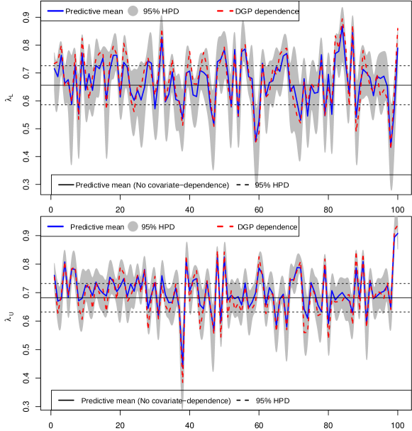
Figure 2: The excerpt summary of the predictive lower tail-dependences (top) and upper tail-dependences (bottom). The predictive lower and upper tail-dependences are calculated from the four-fold cross-validation of two modeling strategies (Joint+CD.+VS. and Joint+Const.). The data consists of $1,000$ observations with $\bar{\bm{\lambda}}_{L}=0.7$ and $\bar{\bm{\lambda}}_{U}=0.7$ as noted in Table  5. The plot only depicts predictive lower and upper tail-dependences for an excerpt of the first 100 observations for better visualization.

6 Application to financial data forecasting

In order to illustrate our method, we apply it to a financial application with daily stock returns. The copula models are reparameterized Joe-Clayton copula, Clayton copula, Gumbel copula, and Student’s t-copula with split-t distributions on the continuous margins. For the discrete case, see the latent variables approach for the Gaussian copula [34] and the extension to a general copula [41].

6.1 The S&P 100 and S&P 600 data

Our data are daily returns from the S&P 100 and S&P 600 daily stock market indices during the period from February 01, 1989 to February 06, 2015 (see Figure 3). The S&P 100 index includes the largest and most established companies in the U.S. and is a subset of the well-known S&P 500 index. The S&P 600 index covers the small capitalization companies which present the possibility of greater capital appreciation, but at greater risk. The S&P 600 index covers roughly three percent of the total US equities market.

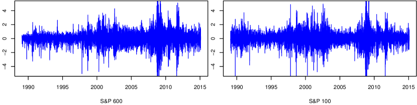
Figure 3: The daily returns of the S&P 600 and S&P 100 indices from February 01, 1989 to February 06, 2015.

Figure 3 shows the time series of the daily returns. It is shown that there is huge volatility in the returns for both the S&P 100 and the S&P 600 during the 2008 financial crisis. Figure 4 depicts six empirical densities for the Return variable that are partitioned into blocks estimated with normal kernel methods by assuming independent observations. The empirical densities in Figure 4 show that the dependences, especially the lower tail-dependence, changes over time. There are signs of extreme positive dependences during the 2008 financial crisis. Figure 4 also suggests that there is a strong lower tail-dependence and upper tail dependence during and after the 2008 financial crisis. The two-parameter Joe-Clayton copula is appropriate for modeling the data without rotation. Furthermore, Joe [20] shows that the usual two-stage approach for copula estimation is not fully efficient for extreme dependences, which is the case in the empirical studies exhibited in Figure 4.

The covariates described in Table 8 in the margins and in the copula features are from nonlinear transformation of historical returns and prices of the series. We standardize each covariate to have zero mean and unit variance. The covariates can be classified into two groups, time-varying variables (RM1, RM5 and RM20) and volatility indicators (CloseAbs95, CloseAbs80, MaxMin95, MaxMin80, CloseSqr95 and CloseSqr80). The reason we use time-varying variables as covariates for modeling tail-dependences is that the empirical study of Patton [33] shows that there exists significant time-varying dependence between the S&P 100 and the S&P 600. Volatility indicators are also used as covariates for measuring tail-dependences because heteroscedasticity is found to be a major source of tail-dependences in stock indices (see the discussion and empirical study in Poon et al. [35] and Hilal et al. [15]). Poon et al. [35] also argues that the choice of volatility indicators is unimportant. Therefore, one can replace the volatility indicators with any other volatility variables, and thus our modeling scheme can be generally applied. The volatility indicators are originally used in Geweke and Keane [14]. Villani et al. [44] and Li et al. [25] apply similar covariates to univariate regression density estimation on the S&P 500 data using mixtures of Gaussian and split-t densities, and they show that those covariates can efficiently capture the volatility in stock indices.

Table 8: Description of covariates used in the model for the S&P 100 and S&P 600 data.

Covariate	Description
Return	Daily return $y_{t}=100\log(p_{t}/p_{t-1})$ where $p_{t}$ is the closing price.
RM1	Return of last day.
RM5	Return of last week.
RM20	Return of last month.
CloseAbs95	Geometrically decaying average of absolute returns $(1-\rho)\sum\nolimits_{s=0}^{\infty}\rho^{s}|y_{t-2-s}|$ with $\rho=0.95$.
CloseAbs80	Geometrically decaying average of past absolute returns with $\rho=0.80$.
MaxMin95	Measure of volatility $(1-\rho)\sum\nolimits_{s=0}^{\infty}\rho^{s}(\log(p_{t-1-s}^{h})-\log(p_{t-1-s}^{l}))$ with $\rho=0.95$, where $p^{h}$ and $p^{l}$ are the highest and lowest prices.
MaxMin80	Measure of volatility with $\rho=0.80$.
CloseSqr95	Geometrically decaying average of returns $((1-\rho)\sum\nolimits_{s=0}^{\infty}\rho^{s}y_{t-2-s}^{2})^{1/2}$ with $\rho=0.95$.
CloseSqr80	Geometrically decaying average of returns with $\rho=0.80$.

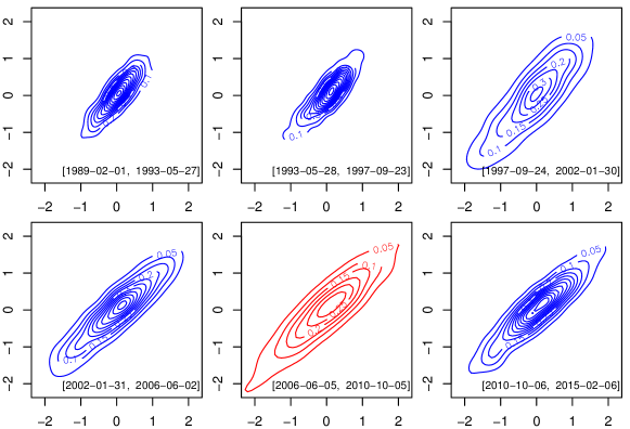
Figure 4: Contour plots for bivariate empirical densities with daily returns of the S&P 100 (y-axis) and the S&P 600 (x-axis) indices from February 01, 1989 to February 06, 2015. The full data are partitioned into six data blocks in chronological order (marked in squared brackets) and the densities are estimated via a normal kernel method within the corresponding blocks. The subplot in the middle of the second row is for the period during the 2008 financial crisis.

6.2 Posterior summary for S&P 100 and S&P 600 data

We firstly present the posterior summary for the Joe-Clayton copula model for S&P 100 and S&P 600 data with split-t margins in two parameterizations in terms of $(\lambda_{L},~{}\lambda_{U})$ in Table 9, and $(\lambda_{L},~{}\tau)$ in Figure 5. The mean posterior acceptance probability is $71\%$. Our MCMC algorithm reduces to the standard Metropolis-Hastings algorithm by setting the number of Newton’s iterations as zero.The MCMC scheme provides a higher posterior acceptance probability and a lower inefficiency factor compared to standard Metropolis-Hastings, where the average acceptance probability is below $20\%$ in our model.

Our marginal models are similar to the model used by Li et al. [25], except that the mean of the split-t is fixed in their model. We focus on explaining the results in the copula component, and one can refer to the work of Li et al. [25] for a detailed interpretation of the marginal models. The variable selection results show that important variables for the lower tail-dependence are RM5 from the S&P 100, CloseAbs95 from the S&P 600, CloseAbs80 from both margins, MaxMin95 from the S&P 100, and CloseSqr95 from both margins. Variables with large posterior inclusion probabilities in the upper-tail dependence are CloseAbs95 from the S&P 100, CloseSqr95 from the S&P 100 and CloseSqr80 from the S&P 600.

The same covariates in the S&P 100 and S&P 600 tend to be highly correlated. The posterior is therefore hard to evaluate using a poorly constructed MCMC algorithm because the likelihood is weakly identified when the same type of covariates in each margin are included in the the copula features. Table 9 shows that when a covariate in one margin is selected in the copula feature, the same covariate in the other margin does not appear in the copula with only two exceptions. This indicates that our variable selection algorithm is efficient in removing superfluous covariates. Also note that the initial values for variable selection indicators are all one. That is, initially, all covariates are included in the model. Our inclusion probabilities for variable selection indicators in Table 9 are very selective in the sense that very few indicators are close to an undecided region around $0.5$, and all of the finally selected variables do not rely on the initially included variables.

Table 9: The summary for the posterior mean values of the Joe-Clayton copula model reparameterized in terms of lower tail-dependence ($\lambda_{L}$) and upper tail-dependence ($\lambda_{U}$) for the S&P 100 and the S&P 600 data from February 01, 1989 to February 06, 2015. In the results for the copula component, the first and second rows for $\beta$ and $\mathcal{I}$ are obtained from the combined covariates that are used in the first and second marginal models. The intercepts are always included in the model. Variables that are selected with an inclusion probability greater than $0.5$ are marked in bold. The average of inefficiency factors for all parameters is $29$. The average acceptance probabilities are all above $0.70$ within each iteration of the Metropolis-Hastings algorithm.

	Intercept	RM1	RM5	RM20	CloseAbs95	CloseAbs80	MaxMin95	MaxMin80	CloseSqr95	CloseSqr80
Marginal component (S&P 600)
$\beta_{\mu}$	$0.146$	$\mathbf{0.120}$	$0.000$	$0.006$	$0.001$	$\mathbf{0.116}$	$-0.001$	$0.002$	$-0.013$	$\mathbf{-0.046}$
$\mathcal{I}_{\mu}$	$1.00$	$\mathbf{1.00}$	$0.01$	$0.22$	$0.02$	$\mathbf{0.96}$	$0.05$	$0.08$	$0.24$	$\mathbf{0.53}$
$\beta_{\phi}$	$-0.318$	$\mathbf{0.041}$	$\mathbf{-0.115}$	$-0.004$	$-0.010$	$-0.012$	$\mathbf{0.217}$	$0.002$	$0.019$	$\mathbf{0.243}$
$\mathcal{I}_{\phi}$	$1.00$	$\mathbf{1.00}$	$\mathbf{1.00}$	$0.16$	$0.13$	$0.17$	$\mathbf{0.94}$	$0.12$	$0.18$	$\mathbf{0.96}$
$\beta_{\nu}$	$1.405$	$0.008$	$\mathbf{-0.230}$	$0.041$	$-0.160$	$-0.098$	$-0.220$	$\mathbf{-0.414}$	$\mathbf{0.428}$	$\mathbf{0.641}$
$\mathcal{I}_{\nu}$	$1.00$	$0.13$	$\mathbf{0.78}$	$0.27$	$0.48$	$0.38$	$0.50$	$\mathbf{0.65}$	$\mathbf{0.56}$	$\mathbf{0.74}$
$\beta_{\kappa}$	$-0.248$	$\mathbf{-0.116}$	$0.000$	$0.000$	$-0.039$	$-0.009$	$-0.057$	$-0.015$	$\mathbf{0.174}$	$-0.003$
$\mathcal{I}_{\kappa}$	$1.00$	$\mathbf{1.00}$	$0.02$	$0.17$	$0.29$	$0.16$	$0.38$	$0.32$	$\mathbf{0.83}$	$0.13$
Marginal component (S&P 100)
$\beta_{\mu}$	$0.091$	$0.000$	$-0.001$	$\mathbf{-0.019}$	$0.010$	$0.000$	$0.011$	$-0.005$	$0.011$	$0.020$
$\mathcal{I}_{\mu}$	$1.00$	$0.02$	$0.05$	$\mathbf{0.57}$	$0.30$	$0.13$	$0.25$	$0.15$	$0.19$	$0.26$
$\beta_{\phi}$	$-0.432$	$-0.001$	$\mathbf{-0.109}$	$\mathbf{-0.026}$	$\mathbf{0.481}$	$\mathbf{-0.191}$	$\mathbf{0.135}$	$0.045$	$\mathbf{-0.477}$	$\mathbf{0.339}$
$\mathcal{I}_{\phi}$	$1.00$	$0.05$	$\mathbf{1.00}$	$\mathbf{0.60}$	$\mathbf{0.96}$	$\mathbf{0.96}$	$\mathbf{0.58}$	$0.33$	$\mathbf{1.00}$	$\mathbf{0.98}$
$\beta_{\nu}$	$0.641$	$-0.024$	$\mathbf{-0.173}$	$0.067$	$-0.151$	$-0.160$	$-0.001$	$0.035$	$-0.005$	$-0.055$
$\mathcal{I}_{\nu}$	$1.00$	$0.20$	$\mathbf{0.62}$	$0.36$	$0.41$	$0.42$	$0.34$	$0.43$	$0.32$	$0.27$
$\beta_{\kappa}$	$-0.140$	$\mathbf{-0.058}$	$0.000$	$-0.005$	$0.033$	$0.000$	$0.020$	$0.000$	$-0.077$	$0.007$
$\mathcal{I}_{\kappa}$	$1.00$	$\mathbf{1.00}$	$0.05$	$0.15$	$0.20$	$0.09$	$0.21$	$0.02$	$0.38$	$0.08$
Copula component ($C$)
$\beta_{\lambda_{L}}$	$0.508$	$0.003$	$-0.017$	$0.000$	$\mathbf{1.497}$	$\mathbf{-0.449}$	$0.031$	$-0.030$	$\mathbf{0.359}$	$0.040$
		$0.001$	$\mathbf{-0.072}$	$0.002$	$0.088$	$\mathbf{0.268}$	$\mathbf{-0.811}$	$0.043$	$\mathbf{-0.498}$	$-0.090$
$\mathcal{I}_{\lambda_{L}}$	$1.00$	$0.07$	$0.42$	$0.00$	$\mathbf{1.00}$	$\mathbf{0.84}$	$0.27$	$0.20$	$\mathbf{0.75}$	$0.37$
		$0.04$	$\mathbf{0.55}$	$0.04$	$0.44$	$\mathbf{0.64}$	$\mathbf{0.96}$	$0.16$	$\mathbf{0.82}$	$0.45$
$\beta_{\lambda_{U}}$	$0.246$	$-0.001$	$-0.001$	$0.000$	$0.044$	$0.001$	$1.384$	$0.005$	$0.199$	$\mathbf{0.347}$
		$-0.001$	$-0.005$	$-0.005$	$\mathbf{-0.887}$	$-0.066$	$-0.466$	$0.226$	$\mathbf{-0.229}$	$-0.157$
$\mathcal{I}_{\lambda_{U}}$	$1.00$	$0.03$	$0.02$	$0.11$	$0.11$	$0.08$	$1.00$	$0.13$	$0.47$	$\mathbf{0.94}$
		$0.02$	$0.09$	$0.36$	$\mathbf{1.00}$	$0.41$	$0.43$	$0.43$	$\mathbf{0.67}$	$0.38$

Figure 5 represents the posterior of marginal features from split-t and copula features, Kendall’s $\tau$ correlation, lower tail-dependence and the derived upper tail dependences between the S&P 100 and the S&P 600, and their 95% HPD. Both the lower and upper tail-dependences are not strong during low volatility periods, but they vary over time significantly. A very high dependence could occur in the tail even though the overall Kendall’s $\tau$ correlation is relatively small.

Figure 6 depicts the contour plot for the posterior density of the Joe-Clayton copula model. The dates selected are based on the ascending order of the estimated lower tail-dependences. We can see that the lower tail-dependence is much higher during the crisis in comparison to the dates before. Also note from the shape of the contour lines that the empirical densities in Figure 4 overestimate the dependences during the non-crisis period and underestimate the tail-dependences during the 2008 financial crisis because they assume temporally independent observations. Our covariate-dependent copula model is capable of capturing the dynamic nature of tail dependences.

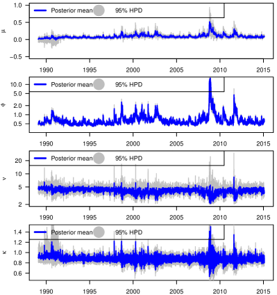
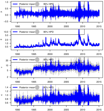
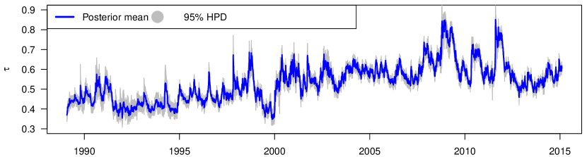
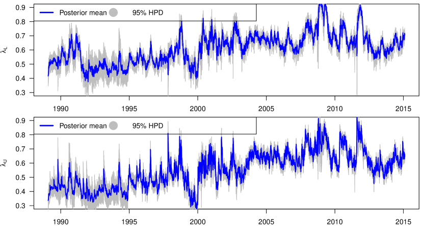
Figure 5: The posterior mean and the 95% highest probability density (HPD) intervals for the Joe-Clayton copula model reparameterized in terms of lower tail-dependence $\lambda_{L}$ and Kendall’s $\tau$ for the S&P 600 and the S&P 100 data from February 01, 1989 to February 06, 2015. The top-left and top-right four subplots show time series of the mean, scale (in log scale), degrees of freedom (in log scale) and skewness features in the margins of the S&P 600 and the S&P 100, respectively. The three subplots at the bottom are the time series for Kendall’s $\tau$, the lower tail-dependence, and the upper tail-dependence $\lambda_{U}$, which is derived based on the posterior of lower tail-dependence and Kendall’s $\tau$.

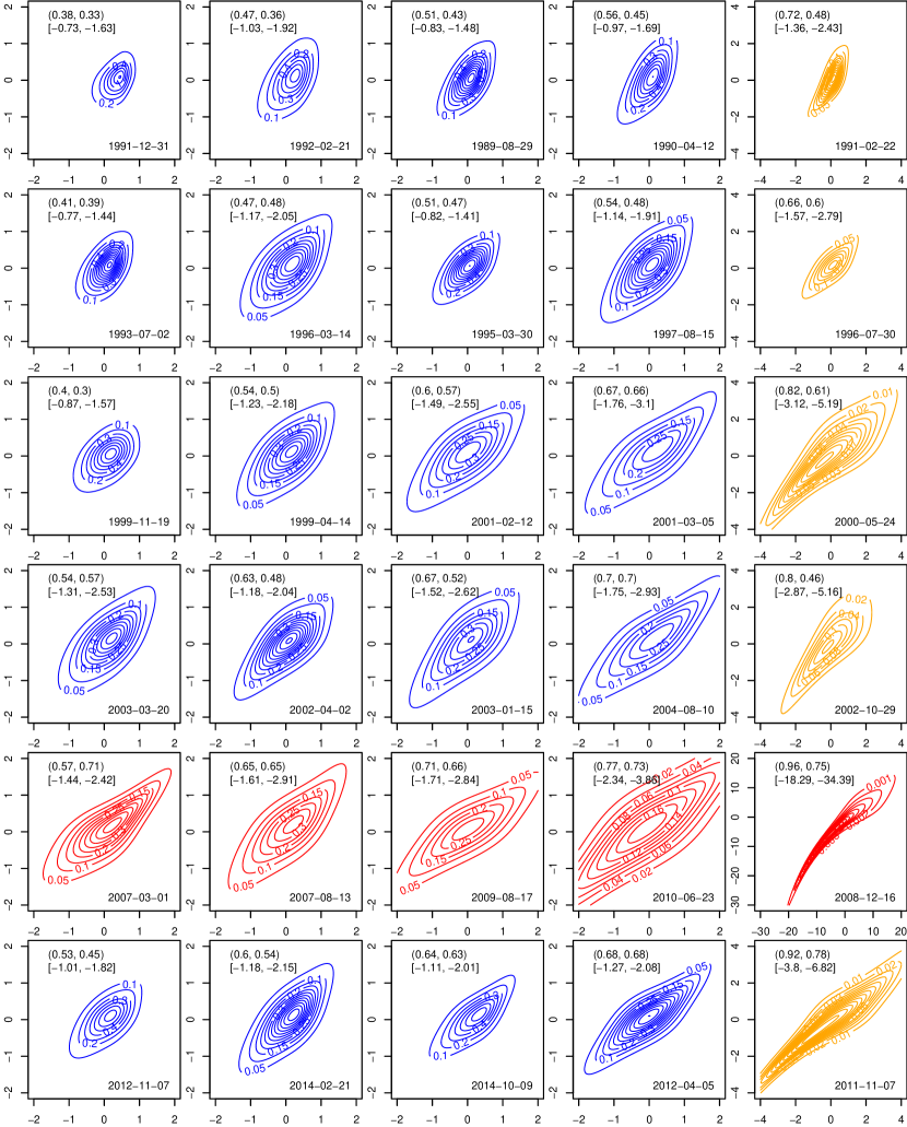
Figure 6: Contour plots of the posterior densities for selected dates with the Joe-Clayton copula model reparameterized in terms of lower tail-dependence $\lambda_{L}$ and upper tail-dependence $\lambda_{U}$ for the S&P 100 (y-axis) and the S&P 600 (x-axis) data from February 01, 1989 to February 06, 2015. The posterior means for $\lambda_{L}$ and $\lambda_{U}$ are marked in round brackets. The 5% VaR and 1% VaR are presented in square brackets. Five days (column-wise view) sorted by ascending order of lower tail-dependences (1%, 25%, 50%, 75% and 99% quantiles) are selected in each data block from the six blocks (row-wise view) used in Figure 4. The subplots in the second last row (highlighted in red) are for the period during the 2008 financial crisis. The magnitudes are enlarged in the subplots of the last column due to the extremely high dependences.

6.3 Forecasting comparisons

In our time series application, we calculate the LPS based on the posterior estimation of 80% of the historical data and the density forecasting of the last 20% of the data. It evaluates the quality of the one-step-ahead predictions using

$$\mathrm{LPS} =\log p(\bm{y}_{(T+1):(T+p)}|\bm{y}_{1:T})$$

$$=\sum\limits_{i=1}^{p}\log\int p(\bm{y}_{T+i}|\{\bm{\beta},\bm{\mathcal{I}}\},\bm{y}_{1:(T+i-1)})p(\{\bm{\beta},\bm{\mathcal{I}}\}|\bm{y}_{1:(T+i-1)})\mathrm{d}\{\bm{\beta},\bm{\mathcal{I}}\},$$

where $\bm{y}_{a:b}$ is the dataset from time $a$ to $b$ and $\{\bm{\beta},\bm{\mathcal{I}}\}$ are the model parameters. This way of calculating LPS is usually computationally costly because every one-step-ahead prediction needs a new posterior sample from the posterior based on the data available at the time of the forecast. We approximate the LPS by assuming that the posterior does not change much as we add a few data points to the estimation sample. Each time we predict 10% of the testing data based on previously estimated posterior by assuming that the observations are independent and then update the posterior. Thus calculating LPS for the whole testing data involves ten times of such a window expanding procedure. Villani et al. [44] documents that this type of approximation is accurate in the application of a smooth mixture of Gaussians for density predictions of the S&P 500 data. Furthermore, with simple algebra, it can be shown that the global LPS in a copula model equals to the sum of the LPS values in each marginal model and the copula component (i.e., $\mathrm{LPS}=\sum\nolimits_{i=1}^{M}\mathrm{LPS}_{i}+\mathrm{LPS}_{C}$). This allows us to parallel compute the LPS values and compare the contributions of different components.

Table 10 shows the out-of-sample comparisons based on LPS of the Joe-Clayton copula, Clayton copula, Gumbel copula and Student’s t-copula in combination with split-t, GARCH(1,1) with normal innovations and SV margins. The specification of the univariate SV model and its MCMC details are described in Kastner and Frühwirth-Schnatter [22]. We apply three modeling strategies (CD.+VS., CD., and Const.) for each reparameterized copula. Both the joint modeling approach and the two-stage approach are applied when possible. For each combination, the global LPS for the full model is decomposed into marginal LPS components ($M_{1}$ and $M_{2}$) and a copula LPS component ($C$).

In the joint approach comparison, the Joe-Clayton copula with covariate-dependent structure and variable selection scheme (CD.+VS.) outperforms the other three copulas that also have the same modeling strategy. The Student’s t-copula with a correlation feature and degrees of freedom modeled with covariate-dependent structure is the second best model, but still falls behind by 36 LPS points. Compared to only modeling constant copula features (Const.), introducing covariate-dependent copula modeling (CD.) improves forecasting performances regarding the global LPS in the four copulas. The improvement is further enhanced when the variable selection scheme is added to the covariate-dependent copula structure (CD.+VS.). Among the four copulas, the Student’s t-copula is the weakest one for modeling tail-dependences in theory because its tail dependences rely on small degrees of freedom. Allowing covariate-dependent structure applied to the degrees of freedom greatly increases the LPS by about $90$ points from $703.96$ to $792.14$.

In the two-stage approach comparison, we compare three types of margins, including the default split-t, GARCH(1,1) and SV margins with a combination of the four copula models with covariate-dependent structure applied to all the copula features. We also calculate the LPS for bivariate DCC-GARCH and bivariate volatility models as benchmarks shown at the bottom of Table 10. The Joe-Clayton copula with split-t margins still performs the best. For the same copula, variable selection significantly improves the forecasting performance in terms of global LPS mainly due to its capacity of preventing overfitting. The GARCH margin and the SV margin fall behind with distinctions in terms of the LPS. Although the bivariate DCC-GARCH does a much better job than bivariate volatility model, with a gap of $269$ LPS points and the bivariate DCC-GARCH also outperforms all of the four copulas with an SV margin and GARCH(1,1) margin, our four covariate-dependent copula models with split-t margins using variable selection outperform the DCC-GARCH with stronger significance of more than $350$ LPS points.

To summarize, copula models with covariate-dependent structure could greatly improve the capacity of capturing tail dependences, and thus they outperform the commonly used volatility models. Joint modeling is more efficient than the two-stage approach. Variable selection is useful in preventing overfitting, which also helps improve the model’s forecasting performances.

Table 10: Model comparison based on LPS. Note that in principle, the global LPS should be equal to the summation of LPS values in the marginal and copula components. But for numerical reasons in MCMC, they are not exactly the same. The numerical standard errors are all below one in all LPS values.

		Reparameterized Copulas
		Joe-Clayton				Clayton				Gumbel				Student’s t-Copula
		CD.+VS.	CD.	Const.		CD.+VS.	CD.	Const.		CD.+VS.	CD.	Const.		CD.+VS.	CD.	Const.
Margins	LPS
		(Joint modeling approach)
SPLIT-t	$M_{1}$	$-1743.12$	$-1745.96$	$-1747.99$		$-1741.04$	$-1805.79$	$-1789.27$		$-1754.36$	$-1756.09$	$-1756.21$		$-1741.47$	$-1859.05$	$-1782.37$
	$M_{2}$	$-1435.98$	$-1430.96$	$-1434.22$		$-1468.25$	$-1589.48$	$-1561.14$		$-1485.68$	$-1549.39$	$-1563.01$		$-1430.07$	$-1516.65$	$-1658.09$
	$C$	$837.50$	$832.63$	$779.14$		$690.22$	$774.34$	$646.57$		$797.78$	$794.91$	$684.60$		$792.14$	$594.60$	$703.96$
	$Global$	$-2344.12$	$-2377.01$	$-2411.06$		$-2523.75$	$-2639.05$	$-2714.69$		$-2448.14$	$-2518.48$	$-2639.58$		$-2380.12$	$-2786.45$	$-2736.49$
		(Two-stage modeling approach)
SPLIT-t	$M_{1}$	$-1740.10$	$-1737.20$	$-1734.57$		$-1741.05$	$-1735.22$	$-1735.81$		$-1737.73$	$-1738.03$	$-1736.72$		$-1741.47$	$-1735.03$	$-1736.18$
	$M_{2}$	$-1428.39$	$-1428.68$	$-1426.78$		$-1436.63$	$-1425.18$	$-1426.63$		$-1427.83$	$-1425.19$	$-1428.41$		$-1433.41$	$-1431.07$	$-1427.53$
	$C$	$819.63$	$225.30$	$121.84$		$694.84$	$262.49$	$121.50$		$781.39$	$621.78$	$129.60$		$788.22$	$553.50$	$289.14$
	$Global$	$-2346.61$	$-2941.80$	$-3045.04$		$-2483.93$	$-2903.64$	$-3043.71$		$-2392.13$	$-2545.14$	$-3036.39$		$-2389.41$	$-2617.19$	$-2883.14$
GARCH(1,1)	$M_{1}$	$-1948.07$	$-1948.07$	$-1948.07$		$-1948.07$	$-1948.07$	$-1948.07$		$-1948.07$	$-1948.07$	$-1948.07$		$-1948.07$	$-1948.07$	$-1948.07$
	$M_{2}$	$-1673.85$	$-1673.85$	$-1673.85$		$-1673.85$	$-1673.85$	$-1673.85$		$-1673.85$	$-1673.85$	$-1673.85$		$-1673.85$	$-1673.85$	$-1673.85$
	$C$	$702.35$	$495.35$	$294.18$		$530.48$	$450.42$	$148.83$		$810.39$	$441.49$	$147.90$		$791.55$	$632.48$	$598.06$
	$global$	$-2919.57$	$-3126.56$	$-3327.73$		$-3091.44$	$-3171.50$	$-3473.09$		$-2811.53$	$-3180.43$	$-3474.01$		$-2830.37$	$-2989.44$	$-3023.86$
SV	$M_{1}$	$-2166.90$	$-2159.29$	$-2178.93$		$-2154.18$	$-2170.90$	$-2194.82$		$-2168.17$	$-2162.75$	$-2168.62$		$-2179.36$	$-2186.61$	$-2183.65$
	$M_{2}$	$-1811.36$	$-1809.61$	$-1814.96$		$-1844.57$	$-1808.54$	$-1787.42$		$-1808.61$	$-1828.60$	$-1824.77$		$-1808.24$	$-1830.06$	$-1826.25$
	$C$	$964.37$	$768.19$	$344.22$		$698.30$	$513.081$	$126.46$		$1012.10$	$733.96$	$231.85$		$1053.19$	$906.58$	$755.63$
	$Global$	$-3013.90$	$-3200.70$	$-3649.67$		$-3300.46$	$-3466.36$	$-3855.78$		$-2964.68$	$-3257.39$	$-3761.53$		$-2934.40$	$-3110.09$	$-3254.27$
		(Bivariate volatility models)
Bivariate DCC-GARCH		$-2730.78$
Bivariate SV		$-2999.63$

6.4 Value-at-Risk comparisons

We also compare the out-of-sample Value-at-Risk for the portfolio of S&P100 and S&P 600 returns with equal weights based on the reparameterized covariate-dependent Joe-Clayton copula, Clayton copula, Gumbel copula models, and the bivariate DCC-GARCH model based on 80% of the historical data in Figure 7. The ratio of violations (RoV) in Figure 7 is the percentage of sample observations lying out of the VaR critical values. Overall, the Joe-Clayton copula captures the extrema most successfully in a time-varying fashion and detects more violations compared to the other methods. The benchmark DCC-GARCH model has the smallest variation in both $5\%$ VaR and $1\%$ VaR compared to other three models, and also has the smallest RoV, which is not suitable to reflect the risk of portfolio returns with time-varying effects. Compared with the Clayton copula and the Gumbel copula, the difference of VaRs in most regions is not obvious except for the volatility periods of mid 2010 and late 2011. In these regions, the $5\%$ VaR and $1\%$ VaR for Gumbel copula overreact to the portfolio’s volatility. From the $5\%$ VaR plot in the top panel of Figure 7, we notice that the Joe-Clayton copula and the Gumbel copula have the same RoV but the VaR for Joe-Clayton copula is more robust than the Gumbel copula. This phenomenon can be seen more clearly in both the periods of mid 2010 and late 2011, when the volatility occurs in portfolio returns.

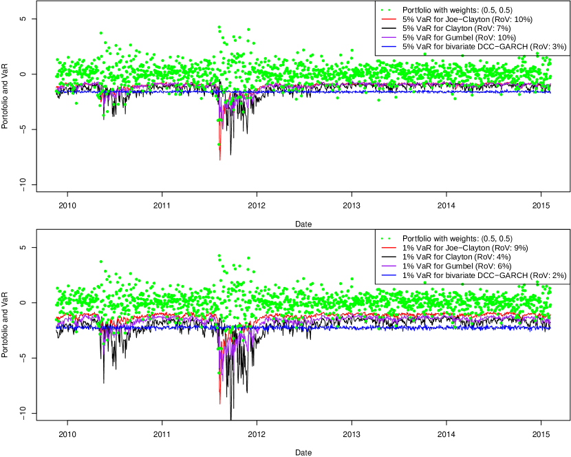
Figure 7: Out-of-sample Value-at-Risk (VaR) for the portfolio of S&P 100 and S&P 600 with equal weights. The 5% (top) and 1% (bottom) VaR are calculated for Joe-Clayton copula, Clayton copula, Gumbel copula, and bivariate DCC-GARCH models based on 80% of the historical data. The ratio of violations (RoV) indicating the percentage of sample observations lying out of the critical values is also reported for each model.

7 Concluding remarks

A general approach for covariate-dependent copula forecasting is proposed. The copula features, as well as the features in the margins are linked to covariates. We use an efficient Bayesian MCMC method to sample the posterior distribution and simultaneously perform variable selection in all components of the model. Both simulation studies and application to the daily returns of the S&P 100 and the S&P 600 indices show the advantages of this approach in terms of understanding the bivariate dependence via known covariates, improving the performances in both tail-dependence forecasting and predictive density forecasting, and evaluating Value-at-Risk. While bivariate applications of copula-based models are still popular, high-dimensional covariate-dependent copula modeling with discrete margins is also a direction for further research by using vine copula constructions or data augmentation such as that exhibited in Pitt et al. [34], Smith and Khaled [41], as well as Panagiotelis et al. [31], but requires further extensive studies.

References

Appendix A New properties of Joe-Clayton copula

The Joe-Clayton copula has some unique attributes. The upper tail-dependence and lower tail-dependence are not functionally dependent. The Clayton copula [Clayton, 1978] and the B5 copula [Joe, 1993] are special cases of the Joe-Clayton copula. All of them belong to a more general class of Archimedean copulas. Furthermore, we also find the following new properties.

1. The inequality holds $0\leq\lambda_{L}\leq 2^{1/2-1/(2\tau)}$ when the lower tail-dependence is not extremely high. We say that $\lambda_{L}$ and $\tau$ are variationally dependent. The proof is non-trivial, but we have verified the inequality numerically in a very careful way. We discover the bound of the inequality through the limit of $\tau(\lambda_{L},\lambda_{U})$ when $\lambda_{U}\to 0$. See Figure 1 for illustration.

2. When $\lambda_{L}\to 0$ (i.e. $\delta\to 0$), we have

   $$\tau\to 1-\frac{2H(2/\theta)-2}{2-\theta}=1-\frac{2H(2\log(2-\lambda_{u})/\log 2)-2}{2-\log 2/\log(2-\lambda_{u})},$$

   and

   $$\frac{\partial\tau}{\partial\theta}\to\frac{2(1-H(2/\theta))}{(\theta-2)^{2}}-\frac{4\psi_{1}(2/\theta+1)}{(\theta-2)\theta^{2}},$$

   where $H(\cdot)$ is the harmonic number. When $\theta\to 2$ (i.e. $\lambda_{U}\to 2-\sqrt{2}\approx 0.59)$, we have $\tau\to 2-\pi^{2}/6\approx 0.36$ and $\partial\tau/\partial\theta\to\pi^{2}/12-Zeta(3)/2\approx 0.22$, where $Zeta(\cdot)$ is the Riemann zeta function. This property allows us to have a more numerically robust posterior inference when a nearly non-dependent situation applies.

3. We also derive the analytical gradients for the copula density with respect to the Kendall’s $\tau$ and tail-dependence of Joe-Clayton copula in B.2, which are used to construct efficient proposal distributions for the MCMC.

The Joe-Clayton copula can only determine positive correlations. If the relationship between two variables is negative, we simply need to rotate the axes of the copula and the estimation procedure remains the same. For example, for copulas rotated by 90 degrees, $u$ has to be set to $1-u$. For 270 degrees, let $v$ be $1-v$. For 180 degrees, set $u$ and $v$ to $1-u$ and $1-v$, respectively. See Durrleman et al. [2000] for the proof that after this transformation, it is still a copula and for other possible transformations to extend the current bivariate copula with more desired properties. In the financial application exhibited in Section 6, the correlations are known to be positive, but modeling negative correlations requires no extra work with our developed R package.

Appendix B The MCMC details

In this section, we briefly present the MCMC details. The MCMC implementation is straightforward, but requires great care of the proposal distribution in the Metropolis–Hastings algorithm.

B.1 The chain rule for the features in copula models

We use the finite-step Newton method embedded in the Metropolis-Hastings algorithm that requires the analytical gradient for the posterior with respect to the features of interest in the marginal and copula components. The chain rule of gradient conveniently modularizes the copula model and reduces the complexity of the gradient calculation.

$$\frac{\partial\log c(u_{1},...,u_{M},\lambda_{L},\tau)}{\partial\lambda_{L}}= \frac{\partial\log c(u_{1},...,u_{M},\theta,\delta)}{\partial\delta}\times\left(\frac{\partial\lambda_{L}}{\partial\delta}\right)^{-1},$$

$$\frac{\partial\log c(u_{1},...,u_{m},\lambda_{L},\tau)}{\partial\tau}= \frac{\partial\log c(u_{1},...,u_{m},\theta,\delta)}{\partial\theta}\times\left(\frac{\partial\tau(\theta,\delta)}{\partial\theta}\right)^{-1},$$

$$\frac{\partial\log c(u_{1},...,u_{M},\lambda_{L},\tau)}{\partial\varphi_{m}}= \frac{\partial\log c(u_{1},...,u_{M},\theta,\delta)}{\partial u_{m}}\times\frac{\partial u_{m}}{\partial\varphi_{m}}+\frac{\partial\log p_{m}(y_{m},\varphi_{m})}{\partial\varphi_{m}},$$

where $\varphi_{m}$ is any feature in the $m$:th marginal density $p_{m}(y_{m},\varphi_{m})$ and $u_{m}$ is the CDF function of its marginal density. The parameters $\theta$ and $\delta$ are the intermediate parameters that link the dependence and correlations with the traditional parametrization for copulas. Particularly, obtaining the gradient for the Student’s t-copula requires the following extra decomposition,

$$\frac{\partial\log c_{t}(u_{1},...,u_{M},\lambda_{L},\tau)}{\partial u_{m}}=\frac{\partial\log p_{t}(x_{1},...,x_{M},\nu)}{\partial x_{m}}/\frac{\partial u_{m}}{\partial x_{m}},$$

where $u_{m}=\int p_{m}(x_{m},\nu)dx_{m}$ are the CDF for univariate Student $t$ density with $\nu$ degrees of freedom in the $m$th margin. Gradients for other elliptical copulas are obtained in a similar way.

The MCMC algorithm requires evaluating $\tau_{\lambda_{L}}^{-1}$ excessively. It can be evaluated numerically or through a dictionary-lookup method. In practice, we have found that the dictionary-lookup method is particularly fast and robust. Modeling the upper tail-dependence can be done in the same manner.

Our model in Section 2 is covariate-dependent. Let $l(\varphi)=x^{\prime}\beta$ be the link function where $\varphi$ is the feature of interest. The gradient expression can be written as

$$\frac{\partial\log c(u_{1},...,u_{M},\varphi)}{\partial\beta}=\frac{\partial\log c(u_{1},...,u_{M},\varphi)}{\partial\varphi}\times\left(\frac{\partial l(\varphi)}{\partial\varphi}\right)^{-1}\times\frac{\partial x^{\prime}\beta}{\partial\beta}.$$

When the conditional link function is used, e.g. $\tau$ depends on $\lambda_{L}$ in our model in the link function $l(\tau|\lambda_{L})=x^{\prime}\beta$, the gradient for $\lambda_{L}$ is slightly more complicated. One needs to write $\tau$ as a function of $\lambda_{L}$ with the link function and substitute it into the copula density. The gradient for $\lambda_{L}$ is obtained thereafter. The details are straightforward, but lengthy, and are omitted here.

B.2 Gradients for features in the Joe-Clayton copula

The gradient for the Joe-Clayton copula w.r.t lower tail-dependence $\lambda_{L}$ can be decomposed as

$$\frac{\partial\log c(u,v,\theta,\delta)}{\partial\delta}= -\log T_{1}(u)-\log T_{1}(v)-\frac{2(1+\delta)\Delta_{1}}{\delta L_{1}}-(\frac{1}{\theta}-2)\frac{\log L_{1}-\delta\Delta_{1}/L_{1}}{\delta^{2}(L_{1}^{1/\delta}-1)}$$

$$+\frac{2\log L_{1}}{\delta^{2}}+\frac{L_{1}^{1/\delta}-(1+\delta)L_{1}^{1/\delta}(\log L_{1}-\delta\Delta_{1}/L_{1})/\delta^{2}-1}{(1+\delta)L_{1}^{1/\delta}-\delta-1/\theta},$$

where $\Delta_{1}=\partial L_{1}/\partial\delta=-T_{1}(u)^{-\delta}\log T_{1}(u)-T_{1}(v)^{-\delta}\log T_{1}(v)$. Furthermore, $\partial\lambda_{L}/\partial\delta=2^{-1/\delta}\log(2)/\delta^{2}.$

The gradient for Joe-Clayton copula with respect to the Kendall’s $\tau$ is decomposed as

$$\frac{\partial\log c(u,v,\theta,\delta)}{\partial\theta}= -(1+\delta)\Delta_{2}(0)+\Delta_{3}(u)+\Delta_{3}(v)+2(1+\delta)\Delta_{2}(-\delta)/L_{1}$$

$$+\frac{(1-2\theta)\Delta_{2}(1/\delta)}{(1-L_{1}^{-1/\delta})\theta\delta}-\frac{\log(1-L_{1}^{-1/\delta})}{\theta^{2}}$$

$$+\frac{(1+\delta)L_{1}^{1/\delta}+\theta(1+\delta)/\delta L_{1}^{1/\delta-1}\Delta_{2}(-1/\delta)-\delta}{(1+\delta)\theta L_{1}^{1/\delta}-\theta\delta-1},$$

where $\Delta_{2}(d)=-T_{1}(u)^{d-1}(1-u)^{\theta}\log(1-u)-T_{1}(v)^{d-1}(1-v)^{\theta}\log(1-v)$ and $\Delta_{3}(s)=\partial\log T_{2}(s)/\partial\theta=(1-s)^{\theta-1}\log(1-s)/T_{2}(s)$. Furthermore,

$$\frac{\partial\tau(\theta,\delta)}{\partial\theta}=\begin{cases}-2/[(\theta-2)^{2}\delta]-8B(2+\delta,2/\theta-1)\left[\theta+\psi(2/\theta-1)-\psi(2/\theta+\delta+1)\right]/(\theta^{4}\delta),\\ \hskip 303.53267pt1\leq\theta<2;\\ -[12+24\psi(1)+6\psi^{2}(1)+\pi^{2}-12(2+\psi(1))\psi(2+\delta)+6\psi^{2}(2+\delta)-6\psi_{1}(2+\delta)]/(24\delta),\\ \hskip 303.53267pt\theta=2;\\ \frac{\left({\begin{array}[]{c}-2(2+\delta)\theta^{4}B(1+\delta+2/\theta,2-2/\theta)-8\pi^{2}(\theta-2)^{2}\cos(2\pi/\theta)/\sin^{2}(2\pi/\theta)\\ -8\pi(\theta-2)^{2}[\psi(1+\delta+2/\theta)-\psi(2-2/\theta)-\theta]/\sin(2\pi/\theta)\end{array}}\right)}{\begin{array}[]{l}\delta(2+\delta)(\theta-2)^{2}\theta^{4}B(1+\delta+2/\theta,2-2/\theta)\end{array}},\\ \hskip 303.53267pt\theta>2,\end{cases}$$

where $\psi_{1}(\cdot)$ is the trigamma function. then gradient for the case $\theta=2$ can be obtained by taking the limiting result from the cases of $1\leq\theta<2$ or $\theta>2$ when $\theta\to 2$,

$$\frac{\partial\tau(\theta,\delta)}{\partial\delta}=\begin{cases}-2/[(\theta-2)\delta^{2}]+4B(2+\delta,2/\theta-1)[\psi(2+\delta)-\psi(2/\theta+\delta+1)-1/\delta]/(\theta^{2}\delta),\\ \hskip 303.53267pt1\leq\theta<2;\\ {}[\psi(2+\delta)-\delta\psi_{1}(2+\delta)-\psi(1)-1]/\delta^{2},{\hskip 147.95424pt}\theta=2;\\ \begin{aligned} -\frac{2}{(\theta-2)\delta^{2}}-\frac{4\pi[\psi(3+\delta)-\psi(2/\theta+\delta+1)-2(1+\delta)/(2\delta+\delta^{2})]}{(2+\delta)\delta\theta^{2}\sin(2\pi/\theta)B(1+\delta+2/\theta,2-2/\theta)},\end{aligned}\\ \hskip 303.53267pt\theta>2.\end{cases}$$

For the Joe-Clayton copula, $u$ and $v$ are exchangeable, and we only present the derivative with respect to $u$:

$$\frac{\partial\log c(u,v,\theta,\delta)}{\partial u}= (1+\delta)\theta\Delta_{4}(0)+(1-\theta)[(1-u)^{\theta-2}/T_{2}(u)+(1-v)^{\theta-2}/T_{2}(v)]$$

$$-2(1+\delta)\Delta_{4}(-\delta)/L_{1}-(1/\theta-2)L_{1}^{-1/\delta-1}\Delta_{4}(-\delta)/(1-L_{1}^{-1/\delta})$$

$$-(1+\delta)\theta L_{1}^{1/\delta-1}\Delta_{4}(-\delta)/\left[(1+\delta)\theta L_{1}^{1/\delta}-\theta\delta-1\right]$$

where $\Delta_{4}(d)=-T_{1}(u)^{d-1}(1-u)^{\theta-1}\theta-T_{1}(v)^{d-1}(1-v)^{\theta-1}\theta$.

B.3 Gradients for features in Student’s t-copula and the covariate-dependent structure

The gradient for the Student’s t-copula w.r.t. the lower tail dependence $\lambda_{Lij}$ for the $i$th and $j$th margins can be obtained via the following chain rule,

$$\frac{\partial\log c_{t}(\bm{u},\lambda_{Lij},\tau)}{\partial\lambda_{Lij}}=\frac{\partial\log p_{t}(\bm{x},\nu,\rho_{ij})}{\partial\nu}/\frac{\partial\lambda_{Lij}}{\partial\nu},$$

where the tail-dependence for $i$th and $j$th margins ($\lambda_{Lij}$) are [Embrechts et al., 1997]

$$\lambda_{Lij}=\frac{\int_{\pi/4-\mathrm{arcsin}(\rho_{ij})/2}^{\pi/2}\mathrm{cos}^{\nu}(t)dt}{\int_{0}^{\pi}\mathrm{cos}^{\nu}(t)dt},$$

where $\rho_{ij}$ is the correlation coefficient for $i$th and $j$th margins.

In a $M$-dimensional Student’s t-copula, the covariate-dependent structure can be conveniently represented in a matrix form as

$$\mathrm{vec}(\bm{T})=l^{-1}([\bm{I}\otimes\bm{X}]\mathrm{vec}\bm{B}),$$

where $\bm{T}$ is a $n\times[M(M-1)/2]$ dependence matrix, $\bm{I}$ is a $M(M-1)/2$ dimensional identity matrix, $\bm{X}$ is the set of covariates used in all marginal models, and $\bm{B}$ is the corresponding coefficient matrix. Other copula features can be linked to covariates in the same way. This representation allows us to jointly estimate the correlation and tail-dependences. Note that there is a curse of dimensionality in higher dimensional modeling with covariate-dependent structures. Currently, limited tests for a smaller number of dimensions (less than $10$) are tried with the Student’s $t$-copula. We find that the computation time dramatically increases as the number of dimension grows.

B.4 Gradients for features in the marginal distributions

The direct derivatives of CDF function and PDF functions with respect to their features are straightforward for most densities. We only document the split-t case for CDF functions. Let $I=\kappa$ if $y>\mu$ and $I=1$ elsewhere, $J=1$, if $y>\mu$ and $J=-1$ elsewhere, and $A=I^{2}\nu\phi^{2}/[(y-\mu)^{2}+I^{2}\nu\phi^{2}]$. The gradient for the split-t CDF function with respect to its features $\mu,\phi,\kappa,\nu$ are as follows,

$$\frac{\partial u_{split-t}(y,\mu,\phi,\kappa,\nu)}{\partial\mu}= -\frac{2I\sqrt{\frac{1}{(y-\mu)^{2}+I^{2}\nu\phi^{2}}}A^{\nu/2}}{(1+\kappa)\text{Beta}\left[\frac{\nu}{2},\frac{1}{2}\right]},$$

$$\frac{\partial u_{split-t}(y,\mu,\phi,\kappa,\nu)}{\partial\phi}= -\frac{2I(y-\mu)\sqrt{\frac{1}{(y-\mu)^{2}+I^{2}\nu\phi^{2}}}A^{\nu/2}}{(1+\kappa)\phi\text{Beta}\left[\frac{\nu}{2},\frac{1}{2}\right]},$$

$$\frac{\partial u_{split-t}(y,\mu,\phi,\kappa,\nu)}{\partial\phi}= \begin{cases}-\frac{\text{Beta}_{R}\left[A,\frac{\nu}{2},\frac{1}{2}\right]}{(1+\kappa)^{2}}&y<\mu\\ -\frac{2(1+\kappa)(y-\mu)\sqrt{\frac{1}{(y-\mu)^{2}+\kappa^{2}\nu\phi^{2}}}A^{\nu/2}+\text{Beta}\left[A,\frac{\nu}{2},\frac{1}{2}\right]}{(1+\kappa)^{2}\text{Beta}\left[\frac{\nu}{2},\frac{1}{2}\right]}&\text{elsewhere,}\end{cases}$$

$$\frac{\partial u_{split-t}(y,\mu,\phi,\kappa,\nu)}{\partial\phi}= \frac{I}{2(1+\kappa)\nu^{2}\text{Beta}\left[\frac{\nu}{2},\frac{1}{2}\right]}\left\{4JA^{\nu/2}{}_{p}F_{q}\left[\left\{\frac{1}{2},\frac{\nu}{2},\frac{\nu}{2}\right\},\left\{1+\frac{\nu}{2},1+\frac{\nu}{2}\right\},A\right]\right.$$

$$\left.+\nu\left(-2(y-\mu)\sqrt{\frac{1}{(y-\mu)^{2}+\kappa^{2}\nu\phi^{2}}}A^{\nu/2}\right.\right.$$

$$-\nu J\text{ Beta}\left[A,\frac{\nu}{2},\frac{1}{2}\right]\left(\log\left(A\right)-\text{$\psi$}\left(\frac{\nu}{2}\right)+\text{$\psi$}\left(\frac{1+\nu}{2}\right)\right)\left.\right.\Bigg{\}},$$

where $\mathrm{Beta}_{R}$ is the regularized beta function, ${}_{p}F_{q}$ is the generalized hypergeometric function.

However, there are exceptions when this derivative is numerically unstable in practice. In this situation, we propose an alternative approach. Note that

$$\frac{\partial u}{\partial\varphi}=\frac{\partial F(y,\varphi)}{\partial\varphi}=\int_{-\infty}^{y}\frac{\partial f(x,\varphi)}{\partial\varphi}\mathrm{d}x,$$

where $u=F(y,\varphi)$ is the CDF function of density $f(y,\varphi)$, and calculating $\partial f(y,\varphi)/\partial\varphi$ is usually easier than $\partial F(y,\varphi)/\partial\varphi$. When the integral cannot be easily obtained analytically, numerical methods can be applied in the last stage.

References

- Aas et al. [2009] Aas, K., Czado, C., Frigessi, A., Bakken, H., Apr. 2009. Pair-copula constructions of multiple dependence. Insurance: Mathematics and Economics 44 (2), 182–198.
- Bollerslev [1986] Bollerslev, T., 1986. Generalized autoregressive conditional heteroskedasticity. Journal of Econometrics 31 (3), 307–327.
- Clayton [1978] Clayton, D., 1978. A model for association in bivariate life tables and its application in epidemiological studies of familial tendency in chronic disease incidence. Biometrika 65 (1), 141–151.
- Czado [2010] Czado, C., 2010. Pair-copula constructions of multivariate copulas. In: Jaworski, P., Durante, F., Härdle, W. K., Rychlik, T. (Eds.), Copula theory and its applications: proceedings of the workshop held in Warsaw, 25-26 September 2009. Springer, pp. 93–109.
- Czado et al. [2012] Czado, C., Schepsmeier, U., Min, A., 2012. Maximum likelihood estimation of mixed c-vines with application to exchange rates. Statistical Modelling 12 (3), 229–255.
- Dobrić and Schmid [2005] Dobrić, J., Schmid, F., 2005. Nonparametric estimation of the lower tail dependence in bivariate copulas. Journal of Applied Statistics 32 (4), 387–407.
- Draisma et al. [2004] Draisma, G., Drees, H., Ferreira, A., De Haan, L., 2004. Bivariate tail estimation: dependence in asymptotic independence. Bernoulli 10 (2), 251–280.
- Durrleman et al. [2000] Durrleman, V., Nikeghbali, A., Roncalli, T., 2000. A simple tranformation of copulas. Working paperGroupe de Recherce Operationelle, Credit Lyonnais, France.
- Embrechts et al. [1997] Embrechts, P., Klüppelberg, C., Mikosch, T., 1997. Modelling extremal events. Vol. 33. Springer Science & Business Media.
- Engle [2002] Engle, R., 2002. Dynamic conditional correlation: A simple class of multivariate generalized autoregressive conditional heteroskedasticity models. Journal of Business & Economic Statistics 20 (3), 339–350.
- García et al. [2013] García, J. E., González-López, V., Nelsen, R., Mar. 2013. A new index to measure positive dependence in trivariate distributions. Journal of Multivariate Analysis 115, 481–495.
- Geweke [2001] Geweke, J., 2001. Bayesian econometrics and forecasting. Journal of Econometrics 100 (1), 11–15.
- Geweke and Amisano [2010] Geweke, J., Amisano, G., 2010. Comparing and evaluating Bayesian predictive distributions of asset returns. International Journal of Forecasting 26 (2), 216–230.
- Geweke and Keane [2007] Geweke, J., Keane, M., 2007. Smoothly mixing regressions. Journal of Econometrics 138 (1), 252–290.
- Hilal et al. [2011] Hilal, S., Poon, S.-H., Tawn, J., Sep. 2011. Hedging the black swan: Conditional heteroskedasticity and tail dependence in S&P500 and VIX. Journal of Banking & Finance 35 (9), 2374–2387.
- Huang et al. [2009] Huang, J.-J., Lee, K.-J., Liang, H., Lin, W.-F., 2009. Estimating value at risk of portfolio by conditional copula-GARCH method. Insurance: Mathematics and economics 45 (3), 315–324.
- Jaworski et al. [2010] Jaworski, P., Durante, F., Härdle, W. K., Rychlik, T., 2010. Copula theory and its applications: proceedings of the workshop held in Warsaw, 25-26 September 2009. Vol. 198. Springer.
- Joe [1993] Joe, H., 1993. Parametric families of multivariate distributions with given margins. Journal of Multivariate Analysis 46 (2), 262–282.
- Joe [1997] Joe, H., 1997. Multivariate models and dependence concepts. Chapman & Hall, London.
- Joe [2005] Joe, H., Jun. 2005. Asymptotic efficiency of the two-stage estimation method for copula-based models. Journal of Multivariate Analysis 94 (2), 401–419.
- Kass [1993] Kass, R., 1993. Bayes factors in practice. Journal of the Royal Statistical Society. Series D (The Statistician) 42 (5), 551–560.
- Kastner and Frühwirth-Schnatter [2014] Kastner, G., Frühwirth-Schnatter, S., 2014. Ancillarity-sufficiency interweaving strategy (asis) for boosting mcmc estimation of stochastic volatility models. Computational Statistics & Data Analysis 76, 408–423.
- Kurowicka and Joe [2010] Kurowicka, D., Joe, H., 2010. Dependence modeling: vine copula handbook. World Scientific.
- Ledford and Tawn [1997] Ledford, A. W., Tawn, J. a., May 1997. Modelling Dependence within Joint Tail Regions. Journal of the Royal Statistical Society: Series B (Statistical Methodology) 59 (2), 475–499.
- Li et al. [2010] Li, F., Villani, M., Kohn, R., 2010. Flexible modeling of conditional distributions using smooth mixtures of asymmetric student t densities. Journal of Statistical Planning and Inference 140 (12), 3638–3654.
- Lucas et al. [2014] Lucas, A., Schwaab, B., Zhang, X., 2014. Conditional euro area sovereign default risk. Journal of Business & Economic Statistics 32 (2), 271–284.
- Mardia and Kent [1979] Mardia, K., Kent, J., 1979. Multivariate analysis. Academic Press, London.
- Melino and Turnbull [1990] Melino, A., Turnbull, S. M., 1990. Pricing foreign currency options with stochastic volatility. Journal of Econometrics 45 (1), 239–265.
- Nelsen [2006] Nelsen, R., 2006. An introduction to copulas. Springer Verlag.
- Nott and Kohn [2005] Nott, D., Kohn, R., 2005. Adaptive sampling for Bayesian variable selection. Biometrika 92 (4), 747–763.
- Panagiotelis et al. [2017] Panagiotelis, A., Czado, C., Joe, H., Stöber, J., 2017. Model selection for discrete regular vine copulas. Computational Statistics & Data Analysis 106, 138–152.
- Patton [2006] Patton, A., 2006. Modelling asymmetric exchange rate dependence. International economic review 47 (2), 527–556.
- Patton [2012] Patton, A., 2012. Copula methods for forecasting multivariate time series. In: Handbook of economic forecasting. Vol. 2. Elsevier Oxford, pp. 899–960.
- Pitt et al. [2006] Pitt, M., Chan, D., Kohn, R., Sep. 2006. Efficient Bayesian inference for Gaussian copula regression models. Biometrika 93 (3), 537–554.
- Poon et al. [2003] Poon, S.-H., Rockinger, M., Tawn, J., 2003. Extreme value dependence in financial markets: Diagnostics, models, and financial implications. The Review of Financial Studies 17 (2), 581–610.
- Richardson and Green [1997] Richardson, S., Green, P., 1997. On Bayesian analysis of mixtures with an unknown number of components (with discussion). Journal of the Royal Statistical Society. Series B. Statistical Methodology 59 (4), 731–792.
- Schmidt and Stadtmuller [2006] Schmidt, R., Stadtmuller, U., Jun. 2006. Non-parametric Estimation of Tail Dependence. Scandinavian Journal of Statistics 33 (2), 307–335.
- Scott et al. [2010] Scott, J. G., Berger, J. O., et al., 2010. Bayes and empirical-bayes multiplicity adjustment in the variable-selection problem. The Annals of Statistics 38 (5), 2587–2619.
- Siburg et al. [2015] Siburg, K. F., Stoimenov, P., Weiß, G. N., 2015. Forecasting portfolio-value-at-risk with nonparametric lower tail dependence estimates. Journal of Banking & Finance 54, 129–140.
- Sklar [1959] Sklar, A., 1959. Fonctions de répartition à n dimensions et leurs marges. Publications de l’Institut de Statistique de L’Université de Paris 8, 229–231.
- Smith and Khaled [2012] Smith, M., Khaled, M., 2012. Estimation of copula models with discrete margins via Bayesian data augmentation. Journal of the American Statistical Association 107 (497), 290–303.
- Smith [2015] Smith, M. S., 2015. Copula modelling of dependence in multivariate time series. International Journal of Forecasting 31 (3), 815–833.
- Tran et al. [2014] Tran, M.-N., Giordani, P., Mun, X., Kohn, R., Pitt, M. K., 2014. Copula-type estimators for flexible multivariate density modeling using mixtures. Journal of Computational and Graphical Statistics 23 (4), 1163–1178.
- Villani et al. [2009] Villani, M., Kohn, R., Giordani, P., Dec. 2009. Regression density estimation using smooth adaptive Gaussian mixtures. Journal of Econometrics 153 (2), 155–173.
- Villani et al. [2012] Villani, M., Kohn, R., Nott, D. J., 2012. Generalized smooth finite mixtures. Journal of Econometrics 171 (2), 121–133.
- Yau et al. [2003] Yau, P., Kohn, R., Wood, S., 2003. Bayesian variable selection and model averaging in high-dimensional multinomial nonparametric regression. Journal of Computational and Graphical Statistics 12 (1), 23–54.
- Yu and Meyer [2006] Yu, J., Meyer, R., 2006. Multivariate stochastic volatility models: Bayesian estimation and model comparison. Econometric Reviews 25 (2-3), 361–384.