Tachyon potentials from a supersymmetric FRW model

Abstract

Considering that the effective theory of closed string tachyons can have worldsheet supersymmetry, as shown by Vafa, we study a worldline supersymmetric action in a FRW background, whose superpotential originates a tachyon scalar potential. There are such potentials with spontaneously broken supersymmetry at the instability and supersymmetric after tachyon condensation. Furthermore, given a tachyonic potential, the superpotential can be computed by a power series ansatz and has a free parameter which can be chosen such that complex solutions become real.

I Introduction

Many phenomena in physics are related to the transition or decay from an unstable state, to other stable one. The corresponding evolution is described frequently by a tachyonic potential, with a ‘negative’ mass term, like in the case of the Higgs potential or in the Landau-Ginzburg theory. String theory has in its lowest mode tachyons. However the inclusion of supersymmetry is consistent because they can be eliminated by the GSO truncation. Nevertheless, a better knowledge of string theory requires the understanding of the unstable configurations, whose evolution can be described by the condensation of the tachyonic modes. The complexity of string theory has made this study rather difficult, and it was first performed in the somewhat simpler instance of open strings, resumed by the well known Sen conjectures sen . For closed strings the situation is more complicated, in particular because it involves the structure of space-time. An interesting fact in this case, is that closed string tachyons, which are nonsupersymmetric in target space, can have worldsheet supersymmetry vafa . In this sense we address the question of supersymmetric tachyons in the simplified framework of a FRW background, with ‘worldline’ local supersymmetry, i.e. the time variable is extended to the superspace of supersymmetry.

Supersymmetric quantum cosmology has been studied in various formulations. As usual for uniform spaces, it has been obtained as the “minisuperspace” formulation ryan of four dimensional supergravity obregon0 , see also eath . The Wheeler-deWitt equation is traced back to the ‘square root’ of the hamiltonian constraint, i.e. the supersymmetric charge constraints. Additionally to these constraints, there are also the Lorentz transformations of the fermionic degrees of freedom obregon0 , which restrict strongly the solutions obregon . An alternative supersymmetrization of these models has been given in superfield , by a ‘worldline’ one-dimensional superfield approach, where the time variable is extended to a (supersymmetry) superspace. This formulation has been worked out systematically for all Bianchi models bianchi , matter has been included as well superfield , see also moniz . We follow an approach of this type, by means of the covariant formulation of one-dimensional supergravity, given by the so called ‘new’ $\Theta$ variables wess ; cupa , which allows in a systematic and straightforward way to write supergravity invariant actions. The fermionic sector of the superfield approach has less components than the one of the reduction of four dimensional supergravity, as it is one dimensional, which is some sense compensates the absence of Lorentz constraints. In fact, in both approaches the wave function of the universe seems to have only two independent components tkachwf ; obregon . However, the complexity of four, or higher dimensional supergravity, has made interesting the study of the worldline superfield approach, which keeps the essence of supersymmetry in a relative simple way.

The action we are considering contains two real scalars, one of them the dilaton, and the other one has a tachyonic potential $V(T)$ zwiebach , coupled to FRW supergravity. We formulate one-dimensional $N=2$ supespace supergravity following cupa and the superfield form of the action is taken from superfield . The final action is obtained after a rescaling and eliminating the auxiliary fields. For completeness we give also the hamiltonian formulation which closes consistently without further complications. As usual in supergravity, the superpotential is related to the scalar potential by a differential equation which is not positive definite. In order to solve this equation, we consider the case $k=0$ and make an ansatz of separation of variables. We look for superpotentials corresponding to tachyonic potentials $V(T)$ and in particular such that both supersymmetries are spontaneously broken at the maximum, and after condensation they are restored. We look also for a general solution of this differential equation by a power series ansatz. With this ansatz, depending on the potential, the superpotential can be complex, with complex values for quantities like the mass. However there is a parameter which can be chosen in such a way that the solutions are real. In the second section of this work we give our start point bosonic action, in the third section we give the one-dimensional superspace supergravity formulation, in the fifth section we give the tachyon action, in the sixth section the hamiltonian is formulated and in the next section we study the solutions for the superpotential, in the last section we sketch conclusions. There are two appendices, the first one on the ‘new’ $\Theta$-variables formulation and in the second one there are details of the power series solutions.

II Closed String Tachyon Effective Action

The closed string tachyon effective action in the bosonic sector is given according to zwiebach as

$$S=\frac{1}{2\kappa_{D}^{2}}\int\sqrt{-g}e^{-2\phi}\left[R+4\left(\partial\phi\right)^{2}-\left(\partial T\right)^{2}-2V(T)\right]d^{D}x,$$ (1)

where $T$ is the closed string tachyon field, $V(T)$ is the tachyon potential and $\phi$ is the dilaton field. This action can be written in the Einstein frame by means of $g_{\mu\nu}^{string}=e^{\phi}g_{\mu\nu}^{Einstein}$, which is more suitable for our cosmological approach. For a four dimensional FRW metric and in the Einstein frame, the Lagrangian takes the form

$$S=\int\left[-\frac{3\dot{a}^{2}a}{\kappa^{2}N}+\frac{3Nka}{\kappa^{2}}+\frac{a^{3}}{\kappa^{2}N}\dot{\phi}^{2}+\frac{a^{3}}{2\kappa^{2}N}\dot{T}^{2}-\frac{a^{3}Ne^{2\phi}V\left(T\right)}{\kappa^{2}}\right]dt,$$ (2)

where $N$ is the lapse function and $a$ is the scale factor. This Lagrangian is invariant (up to a total derivative) under time reparametrizations of the form $t\rightarrow f(t)$. This invariance under time reparametrization is extended to supersymmetry supersymmetry by the introduction of a Grassmann superspace associated to the bosonic time coordinate $t$ (see Tkach et al. in superfield ).

As usual, the Hamiltonian of the bosonic theory, has the form $H=NH_{0}$ where $N$ is the lapse function. Then, the associated equation of motion $\partial H/\partial N=0$ implies the first class constraint

$$H_{0}=-\frac{\kappa^{2}}{12a}\pi_{a}^{2}-\frac{3ka}{\kappa^{2}}+\frac{\kappa^{2}}{4a^{3}}\pi_{\phi}^{2}+\frac{\kappa^{2}}{2a^{3}}\pi_{T}^{2}+\frac{a^{3}e^{2\phi}V(T)}{\kappa^{2}}=0,$$ (3)

where $\pi_{i}$ are the canonical momenta of the coordinates $i=a,T,\phi$.

III Superspace supergravity

Superspace is the natural framework for a geometrical formulation of supersymmetry and supergravity salam . It extends spacetime by anticommuting Grassmann variables, $x^{m}\rightarrow(x^{m},\theta^{\mu})$. The field content of the superfields is given by the Grassmann power expansion in the anticommuting variables $\phi(z)=\sum_{n}1/n!\,\theta^{\mu_{1}}\cdots\theta^{\mu_{n}}\phi_{\mu_{1}\cdots\mu_{n}}(x)$. Supergravity is invariant under local supersymmetry transformations $\xi^{m}\rightarrow\xi^{m}(x)$, $\xi^{\mu}\rightarrow\xi^{\mu}(x)$, where $\xi^{m}$ are spacetime translation and $\xi^{\mu}$ supersymmetry transformation parameters. It can be generalized to superspace diffeomorphisms wess , $z^{M}\equiv(x^{m},\theta^{\mu})\rightarrow{z^{\prime}}^{M}=z^{M}+\xi^{M}(z)$. This generalization actually amounts to introduce additional ‘superspace’ gauge degrees of freedom corresponding to the $\theta$-components of the Grassmann expansion of $\xi^{M}(x,\theta)$. In order to formulate such a theory, the vierbein and spin connection are generalized to superspace tensors, the vielbein ${E_{M}}^{A}(z)$, and the superconnection ${\phi_{MA}}^{B}$, where $A=(a,\alpha)$ are local Lorentz indices and $M=(m,\mu)$ are superspace world indices wess . If $V_{A}$ is a Lorentz supervector, its covariant derivatives are $\mathcal{D}_{A}V_{B}={E_{A}}^{M}(\partial_{M}V_{A}-{\phi_{MB}}^{C}V_{C})$, and satisfy the graded (anti)commutators $[\mathcal{D}_{A},\mathcal{D}_{B}]_{\pm}V_{C}=-{T_{AB}}^{D}\mathcal{D}_{D}V_{C}-{R_{ABC}}^{D}V_{D}$, where ${E_{A}}^{M}(z)$ is the inverse vielbein and the torsion and curvature tensors satisfy the graded Bianchi identitites. For the construction of the lagrangian, in superfield a somewhat adhoc superspace formulation has been proposed. Here we will use the ‘new’ superspace formulation, see Apendix A, which follows from general superspace covariance, by a consistent elimination of the superspace gauge degrees of freedom wess ; new ; cupa , without requiring a gauge fixing. This parametrization corresponds to a field redefinition of the superfield components $\phi_{\mu_{1}\cdots\mu_{n}}(x)\rightarrow\left.\mathcal{D}_{[\alpha_{1}}\cdots\mathcal{D}_{\alpha_{n}]}\phi(z)\right|_{\theta=0}$ and the superfields are given by $\Phi(x,\Theta)=\left.e^{\Theta^{\alpha}\mathcal{D}_{\alpha}}\phi(z)\right|_{\theta=0}$, where $\Theta$ are anticommuting Lorentz spinor variables. Full manifest covariance can be mantained by keeping $\Phi(z,\Theta)=e^{\Theta^{\alpha}\mathcal{D}_{\alpha}}\phi(z)$ and setting $\theta=0$ at the end of the computations. In this formulation, the supergravity multiplet contains the vierbein, the spin conection, and certain components of the curvature and torsion tensors, constrained by the Bianchi identities. In Appendix A this formulation is reviewed, following cupa . Superfields transform by field dependent transformations (49) and covariant derivatives can be defined consistently (53) in such a way that there is a vielbein whose superdeterminant is an invariant density (58) and allows to construct invariant supergravity actions. We use these results for a superspace formulation of one-dimensional supergravity. To set conventions, we first observe that simple one-dimensional supersymmetry has the grassmanian variables $\theta$ and $\bar{\theta}=\theta^{\dagger}$. The integration properties for these variables are $\int d\theta=0$, $\int\theta d\theta=1$. Generic superfields are real and are given by $\phi(t,\theta,\bar{\theta})=A(t)+\theta\psi(t)-\bar{\theta}\bar{\psi}(t)+\theta\bar{\theta}B(t)$, where $A(t)$ and $B(t)$ are real and $\psi^{\dagger}=\bar{\psi}$. The representation of supersymmetric charges is $Q=\frac{d}{d\theta}-i\bar{\theta}\frac{d}{dt}$ and $\bar{Q}=-\frac{d}{d\bar{\theta}}+i\theta\frac{d}{dt}$, which satisfy $\{Q,\bar{Q}\}=2i\frac{d}{dt}$, the covariant derivatives are $D=\frac{d}{d\theta}+i\bar{\theta}\frac{d}{dt}$ and $\bar{D}=-\frac{d}{d\bar{\theta}}-i\theta\frac{d}{dt}$. There are also chiral superfields which are complex and satisfy $\bar{D}\phi=0$, and which in the chiral base have the expansion $\phi(t,\theta)=A(t)+\theta\psi(t)$.

Supergravity in one dimension, as well as gravity, is trivial and there is no curvature tensor, and in a minimal version, the torsion tensor is the same as in flat superspace, i.e. its only non-vanishing component is ${T_{\theta\bar{\theta}}}^{t}=2i$, consistently with the Bianchi identities, as can be easily verified by dimensional reduction from minimal supergravity in four dimensions wess , or by direct computation in one dimension. For the one-dimensional ‘new’ superspace formulation, unlike the appendix A, we will denote $z^{M}=(t,\Theta,\bar{\Theta})$ and for simplicity we will omit the tildes. Thus superfields $\Phi(z)=A(t)+\Theta\chi(t)-\bar{\Theta}\bar{\chi}(t)+\Theta\bar{\Theta}B(t)$ transform as

$$\delta_{\xi}\Phi(z)={\eta_{\xi}}^{M}(z)\partial_{M}\Phi(z)\equiv\xi^{M}(x)\left[\eta_{M}^{\ t}(z)\frac{\partial\Phi(z)}{\partial t}+\eta_{M}^{\ \theta}(z)\frac{\partial\Phi(z)}{\partial\Theta}+\eta_{M}^{\ \bar{\theta}}(z)\frac{\partial\Phi(z)}{\partial\bar{\Theta}}\right],$$ (4)

Thus, from (51) it turns out that

$${\eta_{\xi}}^{t} =-\xi-ie^{-1}\left(\Theta\bar{\zeta}+\bar{\Theta}\zeta\right)+\frac{1}{2}e^{-2}\Theta\bar{\Theta}\left(\bar{\zeta}\psi-\zeta\bar{\psi}\right),$$ (5)

$${\eta_{\xi}}^{\theta} =-\zeta+\frac{i}{2}e^{-1}\left(\Theta\bar{\zeta}+\bar{\Theta}\zeta\right)\psi-\frac{1}{4}e^{-2}\Theta\bar{\Theta}\zeta\psi\bar{\psi},$$ (6)

where the supersymmetry parameters are $\xi^{M}(x)=(\xi^{t},\xi^{\theta},\xi^{\bar{\theta}})\equiv(\xi,\zeta,\bar{\zeta})$ and ${\eta_{\xi}}^{\bar{\theta}}=({\eta_{\xi}}^{\theta})^{\dagger}$. The resulting component transformations are

$$\delta_{\xi}A =-\xi\dot{A}-\zeta\chi+\bar{\zeta}\bar{\chi},$$ (7)

$$\delta_{\xi}\chi =-\xi\dot{\chi}-ie^{-1}\bar{\zeta}\dot{A}+\frac{i}{2}e^{-1}\bar{\zeta}(\psi\chi-\bar{\psi}\bar{\chi})+\bar{\zeta}B,$$ (8)

$$\delta_{\xi}\bar{\chi} =-\xi\dot{\bar{\chi}}+ie^{-1}{\zeta}\dot{A}-\frac{i}{2}e^{-1}{\zeta}(\psi\chi-\bar{\psi}\bar{\chi})+{\zeta}B,$$ (9)

$$\delta_{\xi}B =-\xi\dot{B}-ie^{-1}(\zeta\dot{\chi}+\bar{\zeta}\dot{\bar{\chi}})+\frac{1}{2}e^{-2}\zeta\bar{\psi}(\dot{A}+iB)-\frac{1}{2}e^{-2}\bar{\zeta}\psi(\dot{A}-iB)-\frac{1}{12}e^{-2}(\zeta\chi-\bar{\zeta}\bar{\chi})\psi\bar{\psi},$$ (10)

as well as the one of $\bar{\chi}$, obtained from (8) by complex conjugation. Further, the vielbein corresponding to transformations (4), which transforms as $\delta_{\xi}{\nabla_{M}}^{A}=\partial_{M}\eta_{\xi}^{N}{\nabla_{N}}^{A}+\eta_{\xi}^{N}\partial_{N}{\nabla_{M}}^{A}$, can be obtained from (56)

$${\nabla_{M}}^{A}=\left(\begin{array}[c]{ccc}e+i(\Theta\bar{\Psi}+\bar{\Theta}\psi)&\frac{1}{2}\psi&\frac{1}{2}\bar{\psi}\\ -i\bar{\Theta}&0&-1\\ i\Theta&1&0\end{array}\right),$$ (11)

and from its transformation law we get

$$\delta_{\xi}e =-\frac{d}{dt}(\xi e)+i(\zeta\bar{\psi}+\bar{\zeta}\psi),$$ (12)

$$\delta_{\xi}\psi =-2\frac{d}{dt}\left(\zeta+\frac{1}{2}\xi\psi\right),$$ (13)

which can be verified to be consistent with the usual vielbein transformations wess . The invariant density is obtained as usual from the superdeterminant $\mathcal{E}=\mathrm{Sdet}({\nabla_{M}}^{A})$, and transforms as $\delta_{\xi}\mathcal{E}=(-1)^{m}\partial_{M}(\xi^{M}\mathcal{E})$

$$\mathcal{E}=-e-\frac{i}{2}(\Theta\bar{\Psi}+\bar{\Theta}\psi),$$ (14)

The inverse vielbein can be computed from (11), and from it we get the covariant derivatives which will be needed for the lagrangian of the next section

$$\nabla_{\theta}\Phi =\chi+ie^{-1}\bar{\Theta}\left[\dot{A}-\frac{1}{2}(\psi\chi-\bar{\psi}\bar{\chi})-ieB\right]+e^{-1}\Theta\bar{\Theta}\left(-i\dot{\chi}-\frac{1}{2}e^{-1}\bar{\psi}\dot{A}-\frac{1}{4}e^{-1}\psi\bar{\psi}\chi+\frac{i}{2}\bar{\psi}B\right),$$ (15)

$$\nabla_{\bar{\theta}}\Phi =\bar{\chi}-ie^{-1}\Theta\left[\dot{A}-\frac{1}{2}(\psi\chi-\bar{\psi}\bar{\chi})+ieB\right]+e^{-1}\Theta\bar{\Theta}\left(i\dot{\bar{\chi}}-\frac{1}{2}e^{-1}\psi\dot{A}-\frac{1}{4}e^{-1}\psi\bar{\psi}\bar{\chi}-\frac{i}{2}\psi B\right).$$ (16)

IV Susy Closed Tachyon Model

The supersymmetric cosmological model is obtained upon an extension of the time coordinate into a supermultiplet $t\rightarrow(t,\Theta,\bar{\Theta})$. Due to this time supersymmetric generalization, also the fields of the theory are generalized as superfields, the expansion is given by

$$\begin{array}[c]{c}\mathcal{A}\left(t,\Theta,\bar{\Theta}\right)=a\left(t\right)+i\Theta\bar{\lambda}\left(t\right)+i\bar{\Theta}\lambda\left(t\right)+B\left(t\right)\Theta\bar{\Theta},\\ \mathcal{T}\left(t,\Theta,\bar{\Theta}\right)=T\left(t\right)+i\Theta\bar{\eta}\left(t\right)+i\bar{\Theta}\eta(t)+G\left(t\right)\Theta\bar{\Theta},\\ \Phi\left(t,\Theta,\bar{\Theta}\right)=\phi\left(t\right)+i\Theta\bar{\chi}\left(t\right)+i\bar{\Theta}\chi\left(t\right)+F\left(t\right)\Theta\bar{\Theta},\end{array}$$ (17)

where, $\mathcal{A}$, $\mathcal{T}$ and $\Phi$ are the superfields of $a$, $T$ and $\phi$.

The supersymmetric generalization of the action is given by

$$S=S_{Rsusy}+S_{Msusy},$$ (18)

where, $S_{Rsusy}$ is the cosmological supersymmetric generalization of the free FRW model

$$S_{Rsusy}=\int\left(\frac{3\mathcal{E}}{\kappa^{2}}\mathcal{A}\nabla_{\bar{\theta}}\mathcal{A}\nabla_{\theta}\mathcal{A}-\frac{3\sqrt{k}}{\kappa^{2}}\mathcal{EA}^{2}\right)d\Theta d\bar{\Theta}dt,$$ (19)

and the supersymmetric matter term is

$$S_{Msusy} =\frac{1}{\kappa^{2}}\int\left[-\mathcal{E}\mathcal{A}^{3}\nabla_{\bar{\Theta}}\Phi\nabla_{\Theta}\Phi-\frac{1}{2}\mathcal{EA}^{3}\nabla_{\bar{\Theta}}\mathcal{T}\nabla_{\Theta}\mathcal{T}\right.$$ (20)

$$\left.+\mathcal{EA}^{3}W\left(\Phi,\mathcal{T}\right)\right]d\Theta d\bar{\Theta}dt,$$

where $W\left(\Phi,\mathcal{T}\right)$ is the superpotential. The superpotential expansion can be written as $W\left(\Phi,\mathcal{T}\right)=W(\phi,T)+\frac{\partial W}{\partial\phi}(\Phi-\phi)+\frac{\partial W}{\partial T}(\mathcal{T}-T)+\frac{1}{2}\frac{\partial^{2}W}{\partial T^{2}}(\mathcal{T}-T)^{2}+\frac{1}{2}\frac{\partial^{2}W}{\partial\phi^{2}}(\Phi-\phi)^{2}+\frac{\partial^{2}W}{\partial T\partial\phi}(\mathcal{T}-T)(\Phi-\phi)$. This expansion is finite because the terms $(\mathcal{T}-T)$ and $(\Phi-\phi)$ are purely grassmannian. Upon integration over the Grassmann parameters, we find the supersymmetric cosmological Lagrangian in the gravity sector

$$L_{FRWsusy} =-\frac{3a\dot{a}^{2}}{e\kappa^{2}}+\frac{3ia}{\kappa^{2}}\left(\lambda\dot{\bar{\lambda}}-\dot{\lambda}\bar{\lambda}\right)+\frac{6e\sqrt{k}\lambda\bar{\lambda}}{\kappa^{2}}+\frac{3a\dot{a}}{e\kappa^{2}}\left(\psi\lambda-\bar{\psi}\bar{\lambda}\right)+\frac{3ia\sqrt{k}}{\kappa^{2}}\left(\psi\lambda+\bar{\psi}\bar{\lambda}\right)$$

$$-\frac{3aB^{2}e}{\kappa^{2}}+\frac{6aBe\sqrt{k}}{\kappa^{2}}-\frac{3Be\lambda\bar{\lambda}}{\kappa^{2}}-\frac{3a}{2e\kappa^{2}}\lambda\bar{\lambda}\psi\bar{\psi},$$

the dilaton sector of the matter Lagrangian is given by

$$L_{\phi susy} =\frac{a^{3}\dot{\phi}^{2}}{e\kappa^{2}}+\frac{a^{3}\dot{\phi}}{e\kappa^{2}}\left(\bar{\psi}\bar{\chi}-\psi\chi\right)+\frac{ia^{3}}{\kappa^{2}}\left(\dot{\chi}\bar{\chi}-\chi\dot{\bar{\chi}}\right)+\frac{3ia^{2}\dot{\phi}}{\kappa^{2}}\left(\lambda\bar{\chi}+\bar{\lambda}\chi\right)$$

$$+\frac{a^{3}eF^{2}}{\kappa^{2}}+\frac{3a^{2}eF}{\kappa^{2}}\left(\lambda\bar{\chi}-\bar{\lambda}\chi\right)-\frac{3a^{2}Be\chi\bar{\chi}}{\kappa^{2}}+\frac{a^{3}\chi\bar{\chi}\psi\bar{\psi}}{2e\kappa^{2}}-\frac{6ae\lambda\bar{\lambda}\chi\bar{\chi}}{\kappa^{2}},$$

while for the tachyonic sector we find

$$L_{Tsusy} =\frac{a^{3}\dot{T}^{2}}{2e\kappa^{2}}+\frac{a^{3}\dot{T}}{2e\kappa^{2}}\left(\bar{\psi}\bar{\eta}-\psi\eta\right)+\frac{ia^{3}}{2\kappa^{2}}\left(\dot{\eta}\bar{\eta}-\eta\dot{\bar{\eta}}\right)+\frac{3ia^{2}\dot{T}}{2\kappa^{2}}\left(\lambda\bar{\eta}+\bar{\lambda}\eta\right)$$

$$+\frac{a^{3}eG^{2}}{2\kappa^{2}}+\frac{3a^{2}eG}{2\kappa^{2}}\left(\lambda\bar{\eta}-\bar{\lambda}\eta\right)-\frac{3a^{2}Be\eta\bar{\eta}}{2\kappa^{2}}+\frac{a^{3}\eta\bar{\eta}\psi\bar{\psi}}{4e\kappa^{2}}-\frac{3ae\lambda\bar{\lambda}\eta\bar{\eta}}{\kappa^{2}},$$

and the superpotential term

$$L_{W} =-\frac{6aeW\lambda\bar{\lambda}}{\kappa^{2}}-\frac{3ia^{2}W}{2\kappa^{2}}\left(\bar{\psi}\bar{\lambda}+\psi\lambda\right)-\frac{3a^{2}BeW}{\kappa^{2}}+\frac{3a^{2}eW_{T}}{\kappa^{2}}\left(\bar{\lambda}\eta-\lambda\bar{\eta}\right)$$

$$-\frac{ia^{3}W_{T}}{2\kappa^{2}}\left(\bar{\psi}\bar{\eta}+\psi\eta\right)-\frac{a^{3}eGW_{T}}{\kappa^{2}}+\frac{3a^{2}eW_{\phi}}{\kappa^{2}}\left(\bar{\lambda}\chi-\lambda\bar{\chi}\right)-\frac{ia^{3}W_{\phi}}{2\kappa^{2}}\left(\bar{\psi}\bar{\chi}+\psi\chi\right)$$

$$-\frac{a^{3}eFW_{\phi}}{\kappa^{2}}-\frac{a^{3}e\chi\bar{\chi}W_{\phi\phi}}{\kappa^{2}}+\frac{a^{3}eW_{T\phi}}{\kappa^{2}}\left(\bar{\chi}\eta-\chi\bar{\eta}\right)-\frac{a^{3}e\eta\bar{\eta}W_{TT}}{\kappa^{2}}.$$

Thus the total Lagrangian is

$$L =-\frac{3a\dot{a}^{2}}{e\kappa^{2}}+\frac{3a\dot{a}}{e\kappa^{2}}\left(\psi\lambda-\bar{\psi}\bar{\lambda}\right)+\frac{a^{3}\dot{T}^{2}}{2e\kappa^{2}}-\frac{a^{3}\dot{T}}{2e\kappa^{2}}\left(\psi\eta-\bar{\psi}\bar{\eta}\right)+\frac{3ia^{2}\dot{T}}{2\kappa^{2}}\left(\lambda\bar{\eta}+\bar{\lambda}\eta\right)+\frac{a^{3}\dot{\phi}^{2}}{e\kappa^{2}}$$

$$-\frac{a^{3}\dot{\phi}}{e\kappa^{2}}\left(\psi\chi-\bar{\psi}\bar{\chi}\right)+\frac{3ia^{2}\dot{\phi}}{\kappa^{2}}\left(\lambda\bar{\chi}+\bar{\lambda}\chi\right)+\frac{3ia}{\kappa^{2}}\left(\lambda\dot{\bar{\lambda}}+\bar{\lambda}\dot{\lambda}\right)-\frac{ia^{3}}{2\kappa^{2}}\left(\eta\dot{\bar{\eta}}+\bar{\eta}\dot{\eta}\right)-\frac{ia^{3}}{\kappa^{2}}\left(\chi\dot{\bar{\chi}}+\bar{\chi}\dot{\chi}\right)$$

$$+\frac{6e\sqrt{k}\lambda\bar{\lambda}}{\kappa^{2}}+\frac{3ia\sqrt{k}}{\kappa^{2}}\left(\psi\lambda+\bar{\psi}\bar{\lambda}\right)-\frac{6aeW\lambda\bar{\lambda}}{\kappa^{2}}-\frac{3ia^{2}W}{2\kappa^{2}}\left(\psi\lambda+\bar{\psi}\bar{\lambda}\right)-\frac{ia^{3}W_{T}}{2\kappa^{2}}\left(\psi\eta+\bar{\psi}\bar{\eta}\right)$$

$$+\frac{3a^{2}eW_{T}}{\kappa^{2}}\left(\bar{\lambda}\eta-\lambda\bar{\eta}\right)-\frac{ia^{3}W_{\phi}}{2\kappa^{2}}\left(\psi\chi+\bar{\psi}\bar{\chi}\right)+\frac{3a^{2}eW_{\phi}}{\kappa^{2}}\left(\bar{\lambda}\chi-\lambda\bar{\chi}\right)-\frac{a^{3}eW_{TT}}{\kappa^{2}}\eta\bar{\eta}$$

$$+\frac{a^{3}eW_{T\phi}}{\kappa^{2}}\left(\bar{\chi}\eta-\chi\bar{\eta}\right)-\frac{a^{3}eW_{\phi\phi}}{\kappa^{2}}\chi\bar{\chi}-\frac{3a\psi\bar{\psi}\lambda\bar{\lambda}}{2e\kappa^{2}}+\frac{a^{3}\psi\bar{\psi}\eta\bar{\eta}}{4e\kappa^{2}}+\frac{a^{3}\chi\bar{\chi}\psi\bar{\psi}}{2e\kappa^{2}}-\frac{3ae\lambda\bar{\lambda}\eta\bar{\eta}}{\kappa^{2}}$$

$$-\frac{6ae\lambda\bar{\lambda}\chi\bar{\chi}}{\kappa^{2}}-\frac{3aB^{2}e}{\kappa^{2}}+\frac{6aBe\sqrt{k}}{\kappa^{2}}-\frac{3Be\lambda\bar{\lambda}}{\kappa^{2}}-\frac{3a^{2}Be\eta\bar{\eta}}{2\kappa^{2}}-\frac{3a^{2}Be\chi\bar{\chi}}{\kappa^{2}}-\frac{3a^{2}BeW}{\kappa^{2}}$$

$$+\frac{a^{3}eG^{2}}{2\kappa^{2}}+\frac{3a^{2}eG}{2\kappa^{2}}\left(\lambda\bar{\eta}-\bar{\lambda}\eta\right)-\frac{a^{3}eGW_{T}}{\kappa^{2}}+\frac{a^{3}eF^{2}}{\kappa^{2}}+\frac{3a^{2}eF}{\kappa^{2}}\left(\lambda\bar{\chi}-\bar{\lambda}\chi\right)-\frac{a^{3}eFW_{\phi}}{\kappa^{2}},$$

where the subscripts in $W$ denote partial differentiation with respect to $\phi$ and $T$ respectively. When we perform the variation of the lagrangian with respect to the fields $B$, $F$ and $G$, as usual the following algebraic constraints are obtained,

$$B = \sqrt{k}-\frac{aW}{2}-\frac{1}{2a}\lambda\bar{\lambda}-\frac{1}{4}a\eta\bar{\eta}-\frac{1}{2}a\chi\bar{\chi},$$

$$G = W_{T}-\frac{3}{2a}\left(\lambda\bar{\eta}-\bar{\lambda}\eta\right),$$ (21)

$$F = \frac{W_{\phi}}{2}-\frac{3}{2a}\left(\lambda\bar{\chi}-\bar{\lambda}\chi\right),$$

that is $B$, $F$ and $G$ play the role of auxiliary fields, and they can be solved and eliminated from the lagrangian. When we solve for the auxiliary fields and make the further rescalings $\lambda\rightarrow\kappa a^{-1/2}\lambda$, $\bar{\lambda}\rightarrow\kappa a^{-1/2}\bar{\lambda}$, $\eta\rightarrow\kappa a^{-3/2}\eta$, $\bar{\eta}\rightarrow\kappa a^{-3/2}\bar{\eta}$, $\chi\rightarrow\kappa a^{-3/2}\chi$, $\bar{\chi}\rightarrow\kappa a^{-3/2}\bar{\chi}$, we find the Lagrangian

$$L =-\frac{3a\dot{a}^{2}}{e\kappa^{2}}+\frac{3\sqrt{a}\dot{a}}{e\kappa}\left(\psi\lambda-\bar{\psi}\bar{\lambda}\right)+\frac{3eka}{\kappa^{2}}+\frac{\dot{T}^{2}a^{3}}{2e\kappa^{2}}-\frac{\sqrt{a^{3}}\dot{T}}{2e\kappa}\left(\psi\eta-\bar{\psi}\bar{\eta}\right)+\frac{3i\dot{T}}{2}\left(\lambda\bar{\eta}+\bar{\lambda}\eta\right)$$

$$+\frac{\dot{\phi}^{2}a^{3}}{e\kappa^{2}}-\frac{\sqrt{a^{3}}\dot{\phi}}{e\kappa}\left(\psi\chi-\bar{\psi}\bar{\chi}\right)+3i\dot{\phi}\left(\lambda\bar{\chi}+\bar{\lambda}\chi\right)+3i\left(\lambda\dot{\bar{\lambda}}+\bar{\lambda}\dot{\lambda}\right)-\frac{i}{2}\left(\eta\dot{\bar{\eta}}+\bar{\eta}\dot{\eta}\right)$$

$$-i\left(\chi\dot{\bar{\chi}}+\bar{\chi}\dot{\chi}\right)+\frac{3e\sqrt{k}\lambda\bar{\lambda}}{a}-\frac{3e\sqrt{k}\eta\bar{\eta}}{2a}-\frac{3e\sqrt{k}\chi\bar{\chi}}{a}+\frac{3i\sqrt{ak}}{\kappa}\left(\psi\lambda+\bar{\psi}\bar{\lambda}\right)$$

$$+\frac{3eW^{2}a^{3}}{4\kappa^{2}}-\frac{3e\sqrt{k}a^{2}W}{\kappa^{2}}-\frac{eW_{T}^{2}a^{3}}{2\kappa^{2}}-\frac{eW_{\phi}^{2}a^{3}}{4\kappa^{2}}-\frac{9}{2}eW\lambda\bar{\lambda}+\frac{3}{4}eW\eta\bar{\eta}+\frac{3}{2}eW\chi\bar{\chi}$$

$$-\frac{3ia^{3/2}W}{2\kappa}\left(\psi\lambda+\bar{\psi}\bar{\lambda}\right)-\frac{i\sqrt{a^{3}}W_{T}}{2\kappa}\left(\psi\eta+\bar{\psi}\bar{\eta}\right)+\frac{3eW_{T}}{2}\left(\bar{\lambda}\eta-\lambda\bar{\eta}\right)-\frac{i\sqrt{a^{3}}W_{\phi}}{2\kappa}\left(\psi\chi+\bar{\psi}\bar{\chi}\right)$$

$$+\frac{3eW_{\phi}}{2}\left(\bar{\lambda}\chi-\lambda\bar{\chi}\right)-eW_{TT}\eta\bar{\eta}+eW_{T\phi}\left(\bar{\chi}\eta-\chi\bar{\eta}\right)-eW_{\phi\phi}\chi\bar{\chi}+\frac{3e\kappa^{2}}{4a^{3}}\eta\bar{\eta}\chi\bar{\chi}-\frac{3}{2e}\psi\bar{\psi}\lambda\bar{\lambda}$$

$$+\frac{1}{2e}\psi\bar{\psi}\chi\bar{\chi}+\frac{1}{4e}\psi\bar{\psi}\eta\bar{\eta}.$$

Substituting the equations of motion of the auxiliary fields (21) into the supersymetry transformation of the fermions $\lambda$, $\eta$ and $\chi$ from (8), we get $\delta_{\zeta}\lambda=\bar{\zeta}\left(\sqrt{k}-aW/2\right)+\cdots$, $\delta\eta=\bar{\zeta}W_{T}+\cdots$ and $\delta\chi=\bar{\zeta}W_{\phi}+\cdots$. Therefore, if any the fields on the r.h.s. of these equations has nonvanishing v.e.v., the corresponding fermion is a goldstino and supersymmetry is broken. In the case of $\lambda$, the breaking can be due to the cosmological constant or to a nonvanishing $W$. In fact, if the superpotential has the form $W\sim e^{\phi}f(T)$, as in the examples in the next section, then $W_{\phi}=W$, i.e. $\chi$ contributes to the goldstino if $W\neq 0$.

V Hamiltonian analysis

The canonical momenta are

$$\pi_{a} =-\frac{6a\dot{a}}{e\kappa^{2}}-\frac{3\sqrt{a}\bar{\psi}\bar{\lambda}}{e\kappa}+\frac{3\sqrt{a}\psi\lambda}{e\kappa},$$

$$\pi_{T} =\frac{a^{3}\dot{T}}{e\kappa^{2}}+\frac{\sqrt{a^{3}}\bar{\psi}\bar{\eta}}{2e\kappa}-\frac{\sqrt{a^{3}}\psi\eta}{2e\kappa}+\frac{3a^{3/2}i\lambda\bar{\eta}}{2\sqrt{a^{3}}}+\frac{3a^{3/2}i\bar{\lambda}\eta}{2\sqrt{a^{3}}},$$

$$\pi_{\phi} =\frac{2a^{3}\dot{\phi}}{e\kappa^{2}}+\frac{\sqrt{a^{3}}\bar{\psi}\bar{\chi}}{e\kappa}-\frac{\sqrt{a^{3}}\psi\chi}{e\kappa}+\frac{3a^{3/2}i\lambda\bar{\chi}}{\sqrt{a^{3}}}+\frac{3a^{3/2}i\bar{\lambda}\chi}{\sqrt{a^{3}}},$$

$$\pi_{\lambda} =-3i\bar{\lambda},\text{\ \ }\pi_{\bar{\lambda}}=-3i\lambda,$$

$$\pi_{\eta} =\frac{i}{2}\bar{\eta},\text{\ \ }\pi_{\bar{\eta}}=\frac{i}{2}\eta,$$

$$\pi_{\chi} =i\bar{\chi},\text{\ \ }\pi_{\bar{\chi}}=i\chi.$$

As usual, we can see the appearence of the fermionic constraints

$$\Omega_{\lambda} =\pi_{\lambda}+3i\bar{\lambda},\text{ \ }\Omega_{\bar{\lambda}}=\pi_{\bar{\lambda}}+3i\lambda,$$

$$\Omega_{\eta} =\pi_{\eta}-\frac{i}{2}\bar{\eta},\text{ \ }\Omega_{\bar{\eta}}=\pi_{\bar{\eta}}-\frac{i}{2}\eta,$$ (22)

$$\Omega_{\chi} =\pi_{\chi}-i\bar{\chi},\text{ \ }\Omega_{\bar{\chi}}=\pi_{\bar{\chi}}-i\chi.$$

According to the Dirac formalism, the previous constraints are second class and the dynamics of the system is obtained when we impose the set of constraints (22) and introduce the Dirac brackets, and we obtain

$$\left\{a,\pi_{a}\right\}_{D} =1,\text{ }\left\{\phi,\pi_{\phi}\right\}_{D}=1,\text{ }\left\{T,\pi_{T}\right\}_{D}=1,$$

$$\left\{\lambda,\bar{\lambda}\right\}_{D} =-\frac{1}{6i},\text{ }\left\{\chi,\bar{\chi}\right\}_{D}=-\frac{i}{2},\text{ }\left\{\eta,\bar{\eta}\right\}_{D}=-i.$$ (23)

Using the standard definition for the Hamiltonian and imposing the constraints (22), we can write the Hamiltonian of the theory as

$$H=NH_{0}+\frac{1}{2}\psi S-\frac{1}{2}\bar{\psi}\bar{S},$$ (24)

where

$$\begin{array}[c]{c}H_{0}=-\frac{\kappa^{2}\pi_{a}^{2}}{12a}+\frac{\kappa^{2}\pi_{T}^{2}}{2a^{3}}-\frac{3i\kappa^{2}\pi_{T}}{2a^{3}}\left(\lambda\bar{\eta}+\bar{\lambda}\eta\right)+\frac{\kappa^{2}\pi_{\phi}^{2}}{4a^{3}}-\frac{3i\kappa^{2}\pi_{\phi}}{2a^{3}}\left(\lambda\bar{\chi}+\bar{\lambda}\chi\right)-\frac{3a^{3}}{4\kappa^{2}}W^{2}\\ +\frac{3\sqrt{k}a^{2}}{\kappa^{2}}W-\frac{3ka}{\kappa^{2}}+\frac{a^{3}}{2\kappa^{2}}W_{T}^{2}+\frac{a^{3}}{4\kappa^{2}}W_{\phi}^{2}+\frac{9}{2}W\lambda\bar{\lambda}-\frac{3}{4}W\eta\bar{\eta}-\frac{3}{2}W\chi\bar{\chi}\\ +\frac{3}{2}W_{T}\left(\lambda\bar{\eta}-\bar{\lambda}\eta\right)+\frac{3}{2}W_{\phi}\left(\lambda\bar{\chi}-\bar{\lambda}\chi\right)+W_{TT}\eta\bar{\eta}+W_{T\phi}\left(\chi\bar{\eta}-\bar{\chi}\eta\right)\\ +W_{\phi\phi}\chi\bar{\chi}-\frac{3\sqrt{k}}{a}\lambda\bar{\lambda}+\frac{3\sqrt{k}}{2a}\eta\bar{\eta}+\frac{3\sqrt{k}}{a}\chi\bar{\chi}-\frac{9\kappa^{2}}{2a^{3}}\lambda\bar{\lambda}\chi\bar{\chi}-\frac{9\kappa^{2}}{4a^{3}}\lambda\bar{\lambda}\eta\bar{\eta}-\frac{3\kappa^{2}}{4a^{3}}\eta\bar{\eta}\chi\bar{\chi},\end{array}$$ (25)

$$\begin{array}[c]{c}S=\frac{\kappa\pi_{a}}{\sqrt{a}}\lambda+\frac{\kappa\pi_{T}}{\sqrt{a^{3}}}\eta+\frac{\kappa\pi_{\phi}}{\sqrt{a^{3}}}\chi-\frac{6i\sqrt{ak}}{\kappa}\lambda+\frac{3i\sqrt{a^{3}}}{\kappa}W\lambda\\ +\frac{i\sqrt{a^{3}}}{\kappa}W_{T}\eta+\frac{i\sqrt{a^{3}}}{\kappa}W_{\phi}\chi+\frac{3i\kappa}{2a^{3/2}}\lambda\eta\bar{\eta}+\frac{3i\kappa}{a^{3/2}}\lambda\chi\bar{\chi},\end{array}$$ (26)

$$\begin{array}[c]{c}\bar{S}=\frac{\kappa\pi_{a}}{\sqrt{a}}\bar{\lambda}+\frac{\kappa\pi_{T}}{\sqrt{a^{3}}}\bar{\eta}+\frac{\kappa\pi_{\phi}}{\sqrt{a^{3}}}\bar{\chi}+\frac{6i\sqrt{ak}}{\kappa}\bar{\lambda}-\frac{3i\sqrt{a^{3}}}{\kappa}W\bar{\lambda}\\ -\frac{i\sqrt{a^{3}}}{\kappa}W_{T}\bar{\eta}-\frac{i\sqrt{a^{3}}}{\kappa}W_{\phi}\bar{\chi}-\frac{3i\kappa}{2a^{3/2}}\bar{\lambda}\eta\bar{\eta}-\frac{3i\kappa}{a^{3/2}}\bar{\lambda}\chi\bar{\chi},\end{array}$$ (27)

satisfy the Dirac algebra $\{S,\bar{S}\}_{D}=2H_{0}$, $\{H_{0},S\}_{D}=\{H_{0},\bar{S}\}_{D}=0$.

VI Superpotential solutions

From the $H_{0}$, (25), we identify the scalar potential

$$U(a,\phi,T)=-\frac{3k}{a^{2}}+e^{2\phi}V(T),$$ (28)

which is related to the superpotential $W(\phi,T)$ by

$$U=-\frac{3W^{2}}{4}+\frac{3\sqrt{k}}{a}W-\frac{3k}{a^{2}}+\frac{1}{4}\left(\frac{\partial W}{\partial\phi}\right)^{2}+\frac{1}{2}\left(\frac{\partial W}{\partial T}\right)^{2}.$$ (29)

The form of the scalar potential (28) of a FRW geometry is consistent with $k=0$, hence we restrict ourselves to this geometry, and we get the equation

$$e^{2\phi}V(T)=-\frac{3W^{2}}{4}+\frac{1}{4}\left(\frac{\partial W}{\partial\phi}\right)^{2}+\frac{1}{2}\left(\frac{\partial W}{\partial T}\right)^{2}.$$ (30)

This suggest us a separation of variables of the form $W(\phi,T)=\frac{1}{\sqrt{2}}e^{\phi}f(T)$. With this ansatz we obtain the following relation between the tachyon potential and the tachyonic component of the superpotential

$$(f^{\prime})^{2}-f^{2}=V(T),$$ (31)

where the prime denotes differentiation with respect to $T$. In order to find solutions to this equation we must fix the function $V\left(T\right)$. For example if $V(T)=0$, the solution is $f(T)=e^{T}$. Further, for

$$V(T)=\frac{m^{2}}{2}\left(-T^{2}+\frac{1}{4}T^{4}\right),$$ (32)

which according to the analysis of Zwiebach et.al., produces a big crunch scenario as the final state of the universe zwiebach , there is an imaginary solution $f(T)=imT^{2}/({2\sqrt{2}})$, whose superpotential is

$$W(T)=\frac{i}{4}me^{\phi}T^{2},$$ (33)

which generates complex fermion masses. However, as we show in Appendix B, there is also a real solution given by an infinite power series, which can be written as (63),

$$W(T)=\frac{1}{\sqrt{2}}e^{\phi}\left\{e^{T}-\frac{1}{12}m^{2}T^{3}\left[1-\frac{1}{2}T+\frac{1}{20}\left(1+\frac{3}{2}m^{2}\right)T^{2}+\mathcal{O}(T^{3})\right]\right\}.$$ (34)

Other proposal are potentials of the form $V(T)=\exp(\nu T)$ zwiebach , they are known to prevent the tachyon from reaching infinity in certain cases, with $\nu\geq 2$ there is no initial (positive) tachyon velocity for which the tachyon can reach $T=\infty$. For this potential we find $f(T)=\pm 2(\nu^{2}-4)^{-1/2}\exp(\nu T/2)$, and the superpotential is in this case

$$W(\phi,T)=\pm\frac{2}{\sqrt{\nu^{2}-4}}\exp\left(\phi+\frac{\nu}{2}T\right),\text{ }\nu\neq 2.$$ (35)

Another interesting proposal is for instance

$$W(\phi,T)=e^{\phi}f(T)=\frac{ie^{\phi}[(T-\tau)(\tau+T)+2]}{2\tau^{2}},$$ (36)

as in the case of eq. (33) this superpotential generates complex fermion masses, however it can be made to be real in complete analogy with (34). The tachyon potential corresponding to (36) is

$$V(T)=\frac{1}{4\tau^{4}}\left[\left(\tau^{2}-2\right)^{2}+T^{4}-2\tau^{2}T^{2}\right],$$ (37)

this potential, shown in Fig. 1, has a maximum at $T=0$, with $V(0)=1/4-1/\tau^{2}+1/\tau^{4}$, and minima at $T=\pm\tau$, with $V(\tau)=V(-\tau)=-1/\tau^{2}+1/\tau^{4}$, it also holds that $V(0)-V(\pm\tau)=1/4$, thus if we let $\tau\to\infty$ the potential difference will remain the same, as in the case of Sen’s conjectures.

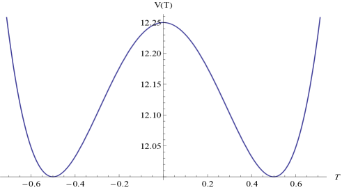
Figure 1: Tachyon potential V(T) from eq. (37) for $\tau=1/2$.

If we compute the superpotential corresponding to (37) following Appendix B, it can be shown that $W_{T}(\phi,0)=e^{\phi}\sqrt{4(1-\tau^{2})+\tau^{4}(A^{2}-1)}/\tau^{2}$, where $A=f(0)$. Further, at the minimum, i.e. at $T=\tau$, we make the power expansion around this point and we get $W_{T}(\phi,\tau)=e^{\phi}\sqrt{4(1-\tau^{2})+\tau^{4}(B^{2}-2)}/\tau^{2}$, where $B=f(\tau)$. If we take the limit $\tau\to\infty$, in order to make the computation we set $u=1/T$ and $\vartheta=1/\tau$ and evaluate the result first at $u=0$ and then we set $\vartheta=0$, we get $W_{T}(\phi,u)|_{u=0,\vartheta=0}=e^{\phi}\sqrt{C^{2}-1}$, where $C=f(u)_{u=0,\vartheta=0}$. Thus if we set $C=1$, the minimum in this limit is supersymmetric. In the limit $\tau\to\infty$ we have also $W_{T}(\phi,T)|_{T=0}=e^{\phi}\sqrt{A^{2}-1}$

hence it does not vanish and supersymmetry is broken. Further, for $T=\tau$ we can make the power series ansatz in the neighborhood of this value, and we get $W_{T}(\phi,\tau)=b$, where $b$ is another constant and it can be easily seen that if $b=0$, the whole power series tends to zero when $\tau\to\infty$, i.e. in this limit $W_{T}(\phi,T)=0$ and supersymmetry is conserved.

An interesting question regards potentials with suitable supersymmetric properties, of the type of Sen conjectures. For instance the potential

$$V(T)=\exp(-nT)\left[\alpha_{0}+\alpha_{1}T+\alpha_{2}T^{2}+\alpha_{3}T^{3}+\alpha_{4}T^{4}\right],$$ (38)

in this case we have $f(T)=(a+bT+cT^{2})\exp\left(-nT/2\right)$ from which we obtain

$$W(T,\phi)=(a+bT+cT^{2})\exp\left(\phi-nT/2\right),$$ (39)

the explicit coefficients $\alpha_{i}$ depend on the free parameters $a$, $n$ and $V_{0}$, in fact we demand the presence of a maximum for $T=0$, this provides us with two equations which can be solved for $b$ and $c$ in (39) and with the condition $V(0)<0$, details of the calculations are given in Appendix (C), see Fig. 2.

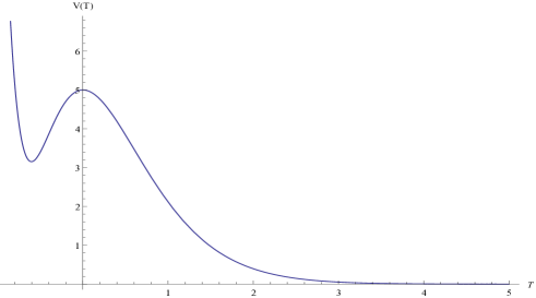
Figure 2: Tachyon potential V(T) produced by $f(T)$ in (64) for $a=10$, $n=3$ and $V_{0}=5$.

At the maximum of this potential $W_{T}(0,\phi)\neq 0$ and $W_{\phi}(0,\phi)\neq 0$, hence supersymmetry is broken. Further, after condensation supersymmetry is restored because $W_{T}\to 0$ and $W_{\phi}\to 0$, when $T\to\infty$.

VII Conclusions

We have studied a worldline supersymmetric theory in a FRW background, with a closed string tachyon. We have constructed the action in the formalism of the ‘new’-$\Theta$ variables in one dimension, which allows systematically to construct supergravity actions. We consider the solutions for the differential equation of the superpotential for given tachyonic potentials and we have obtained solutions with broken supersymmetry at the unstable, tachyonic, configuration, and supersymmetric at the stable minimum. Furthermore, the superpotentials can have simple forms, but which correspond to complex fermionic masses. These superpotentials can be obtained as well by a power series ansatz, whose general solution depends on a real parameter which can be chosen such that the complex solutions can be mapped to real solutions. Some of these potentials have been considered in cosmological models, like in zwiebach where inflationary and big crunch sceneries are given, and it would be interesting to consider the supersymmetric versions.

Acknowledgments

We thank BUAP-VIEP and PIFI-SEP for the support, V. Vázquez-Báez thanks CONACyT for the studies grant during this work.

Appendix A Superspace supergravity

In this appendix we shortly review the ‘new’ superspace formulation of supergravity following cupa . Superfields are defined as

$$\phi(z)\rightarrow\Phi(z)=e^{\Theta^{\alpha}\mathcal{D}_{\alpha}}\phi(z)|_{\theta=0},$$ (40)

where $\Theta$ are anticommuting Lorentz ($SL(2,C)$) covariant spinorial variables. In order to ensure full covariance for these new superfields, the hole “old” superspace can be kept, setting $\theta=0$ at the end of the computations, i.e. $\Phi(z,\Theta)=e^{\Theta^{\alpha}\mathcal{D}_{\alpha}}\phi(z)$.

The preceding redefinition of superfields is complemented by the usual redefinition of local supersymmetry transformations in such a way that Lorentz covariance is kept. The way is to add a local Lorentz transformation to the local superspace translations as followswztrafo :

$$\delta_{\xi}\phi_{A}(z)=-\xi^{B}{E_{B}}^{M}\left(\partial_{M}\phi_{A}-{\phi_{MA}}^{B}\phi_{B}\right)=-\xi^{B}\mathcal{D}_{B}\phi_{A}(z),$$ (41)

hence the new superfields, whose components are Lorentz covariant, transform as $\delta_{\xi}\Phi(z,\Theta)=-\xi^{A}\mathcal{D}_{A}\Phi(z,\Theta)$, i.e.

$$\delta_{\xi}\Phi_{A}(z,\Theta)=-\xi^{B}\mathcal{D}_{B}\phi_{A}-\Theta^{\beta}\xi^{B}\mathcal{D}_{B}\mathcal{D}_{\beta}\phi_{A}-\frac{1}{2}\Theta^{\beta_{1}}\Theta^{\beta_{2}}\xi^{B}\mathcal{D}_{B}\mathcal{D}_{\beta_{1}}\mathcal{D}_{\beta_{2}}\phi_{A}+\dots$$ (42)

The computation of this expression is done taking into account the fact that the multiple covariant derivatives arising from the exponential in (40) appear as fully antisymmetrized products. Thus, when a further derivative is applied on this product, the result must be antisymmetrized, e.g.

$$\mathcal{D}_{\alpha}\mathcal{D}_{\beta}\phi_{A}={\frac{1}{2}}\{\mathcal{D}_{\alpha},\mathcal{D}_{\beta}\}\phi_{A}+{\frac{1}{2}}[\mathcal{D}_{\alpha},\mathcal{D}_{\beta}]\phi_{A}=-{T_{\alpha\beta}}^{C}\mathcal{D}_{C}\phi_{A}-{R_{\alpha\beta A}}^{B}\phi_{B}+\mathcal{D}_{[\alpha}\mathcal{D}_{\beta]}\phi_{A},$$ (43)

where the last term is precisely the second order term of $\Phi(z,\Theta)$. Following these lines, it can be shown that (42) can be cast into the form

$$\delta_{\xi}\Phi_{A}(z,\Theta)={\eta_{\xi}}^{\alpha}(z,\Theta){\frac{\partial}{{\partial\Theta^{\alpha}}}}\Phi_{A}(z,\Theta)+{\eta_{\xi}}^{a}(z,\Theta)\mathcal{D}_{a}\Phi_{A}(z,\Theta)+{\eta_{\xi A}}^{B}(z,\Theta)\Phi_{B}(z,\Theta),$$ (44)

where the coefficients ${\eta_{\xi}}^{A}(z,\Theta)$ and ${\eta_{\xi A}}^{B}(z,\Theta)$ depend on components of the curvature and torsion tensors and their covariant derivatives.

In order to have a geometric formulation in the new superspace, following the Wess-Zumino gauge wzgauge , which eliminates the gauge degrees of freedom introduced by the generalization of local supersymmetry to superspace diffeomorphisms, a new vielbein is introduced. Let us consider a vector field $V_{m}={E_{m}}^{a}V_{a}+{E_{m}}^{\alpha}V_{\alpha}$, this relation can be inverted to

$$V_{a}=E_{\quad a}^{(-1)m}(V_{m}-{E_{m}}^{\alpha}V_{\alpha})=\tilde{E}_{a}^{\ \tilde{M}}V_{\tilde{M}},$$ (45)

where the indices $\tilde{M}\equiv(m,\alpha)$ contain a spacetime world index and a spinorial local index, i.e. $\tilde{E}_{a}^{\ \tilde{M}}=(\tilde{E}_{a}^{\ m},\tilde{E}_{a}^{\ \alpha})\equiv(E_{\quad a}^{(-1)m},-E_{\quad a}^{(-1)m}{E_{m}}^{\alpha})$. With this definition and $\tilde{E}_{\alpha}^{\ \tilde{M}}=\delta_{\alpha}^{\ \tilde{M}}$, an inverse vielbein $\tilde{E}_{A}^{\ \tilde{M}}$ can be defined. The corresponding vielbein is then

$${\tilde{E}_{\tilde{M}}}^{\ \ B}=\left(\begin{array}[c]{ll}{E_{m}}^{\,b}&{E_{m}}^{\,\beta}\\ 0&{\delta_{\alpha}}^{\,\beta}\end{array}\right),$$

i.e. $\tilde{E}_{A}^{\ \tilde{M}}{\tilde{E}_{\tilde{M}}}^{\ \ B}=\delta_{A}^{\ B}$ and ${\tilde{E}_{\tilde{M}}}^{\ \ A}\tilde{E}_{A}^{\ \tilde{N}}=\delta_{\tilde{M}}^{\ \tilde{N}}$. Even if this vielbein seems to correspond to the Wess-Zumino gauge, full covariance can be kept by considering certain components of the torsion and curvature as independent degrees of freedom of the supergravity multiplet. If we define in this basis covariant derivatives as usual by $\mathcal{D}_{A}V_{\tilde{M}}=(-1)^{(m+b)a}{\tilde{E}_{\tilde{M}}}^{\ \ B}\mathcal{D}_{A}V_{B}$ and $\mathcal{D}_{A}V^{\tilde{M}}=\mathcal{D}_{A}V^{B}{\tilde{E}_{B}^{\ \tilde{M}}}$, then

$$[\mathcal{D}_{\tilde{M}},\mathcal{D}_{\tilde{N}}]_{\pm}V_{A}=-{T_{\tilde{M}\tilde{N}}}^{\tilde{P}}\mathcal{D}_{\tilde{P}}V_{A}-{R_{\tilde{M}\tilde{N}A}}^{B}V_{B},$$ (46)

which supplemented by the corresponding Bianchi identities, contains all the information of supergravity. As (46) does not contain derivatives of the old $\theta$-variables, the different levels in the $\theta$-expansion decouple, and the limit $\theta^{\mu}=0$ does not require gauge fixing. Actually, supergravity transformations can be written as $\delta_{\xi}\Phi(z,\Theta)=-\tilde{\xi}^{\tilde{M}}\tilde{\mathcal{D}}_{\tilde{M}}\Phi(z,\Theta)$ and following the same lines as for (44) we get

$$\delta_{\xi}\Phi(z,\Theta)=\left[{\tilde{\eta}_{\xi}}^{\ \alpha}(z,\Theta){\frac{\partial}{{\partial\Theta^{\alpha}}}}+{\tilde{\eta}_{\xi}}^{\ m}(z,\Theta)\mathcal{D}_{m}\right]\Phi(z,\Theta).$$ (47)

Further, the covariant derivative $\mathcal{D}_{m}$ on the r.h.s. of this expression acts on the components of the superfield $\Phi(z,\Theta)$ as in (42), which can be written as

$$\mathcal{D}_{m}\Phi(z,\Theta) ={\partial}_{m}\phi+\Theta^{\beta}({\partial}_{m}-\omega_{m\beta}^{\ \ \ \gamma})\mathcal{D}_{\gamma}\phi-\frac{2}{2}\Theta^{\beta_{1}}\Theta^{\beta_{2}}({\partial}_{m}-\omega_{m\beta_{1}}^{\ \ \ \gamma})\mathcal{D}_{\gamma}\mathcal{D}_{\beta_{2}}\phi+\dots$$

$$={\partial}_{m}\Phi(z,\Theta)+\Theta^{\beta}\omega_{m\beta}^{\ \ \ \gamma}\partial_{\gamma}\Phi(z,\Theta).$$ (48)

Therefore, including a Lorentz index, (47) can be written as

$$\delta_{\xi}\Phi_{A}(z,\Theta)={\hat{\eta}_{\xi}}^{\ \tilde{M}}(z,\Theta)\partial_{\tilde{M}}\Phi_{A}(z,\Theta)+{\hat{\eta}_{\xi A}}^{\ \ B}(z,\Theta)\Phi_{B}(z,\Theta),$$ (49)

where $\hat{\eta}_{\xi}^{\ \alpha}=\tilde{\eta}_{\xi}^{\ \alpha}-\tilde{\eta}_{\xi}^{\ m}\Theta^{\beta}\phi_{m\beta}^{\ \ \ \alpha}$, ${\hat{\eta}_{\xi}}^{\ m}={\tilde{\eta}_{\xi}}^{\ m}$ and ${\hat{\eta}_{\xi A}}^{\ \ B}$ is Lie algebra valued. Further, ${\tilde{\eta}_{\xi}}^{\tilde{M}}=\tilde{\xi}^{\tilde{N}}{\tilde{\eta}_{\tilde{N}}}^{\tilde{M}}$ and ${\tilde{\eta}_{m}}^{\tilde{N}}={\delta_{m}}^{\tilde{N}}$, ${\tilde{\eta}_{mD}}^{\ \ \ B}=0$ and ${\tilde{\eta}}_{\alpha}^{\prime{\tilde{N}}}={\tilde{\eta}}_{\alpha}^{\tilde{N}}-\delta_{\alpha}^{\tilde{N}}$ can be obtained from the following recursion relation

$$\left(1+\Theta^{\beta}\frac{\partial}{\partial\Theta^{\beta}}\right){\tilde{\eta}}_{\alpha}^{\prime{\tilde{N}}}=\Theta^{\beta}\mathcal{D}_{\beta}{\tilde{\eta}}_{\alpha}^{\tilde{N}}+\Theta^{\alpha_{1}}\left(-\Theta^{\alpha_{2}}{R_{\alpha_{2}\alpha\alpha_{1}}}^{\tilde{N}}+{T_{\alpha\alpha_{1}}}^{\tilde{L}}{\tilde{\eta}}_{\tilde{L}}^{\tilde{N}}\right)$$

$$+{\tilde{\eta}}_{\alpha}^{m}\Theta^{\alpha_{1}}\left(-\Theta^{\alpha_{2}}{R_{\alpha_{2}m\alpha_{1}}}^{\tilde{N}}+{T_{m\alpha_{1}}}^{\tilde{L}}{\tilde{\eta}}_{\tilde{L}}^{\tilde{N}}\right)-{{\tilde{\eta}}_{\alpha}}^{\prime\gamma}{{\tilde{\eta}}_{\gamma}}^{\prime{\tilde{N}}},$$ (50)

and a similar one for ${\tilde{\eta}_{\xi A}}^{\ \ B}$. It turns out that

$${\tilde{\eta}_{\xi}}^{\ \tilde{M}}(z,\Theta) =-\tilde{\xi}^{\tilde{M}}+\Theta^{\gamma}\left(\frac{1}{2}\tilde{\xi}^{\beta}{T_{\gamma\beta}}^{\tilde{M}}+\tilde{\xi}^{n}{\phi_{n\gamma}}^{\tilde{M}}\right)$$

$$-\frac{1}{2}\Theta^{\gamma}\Theta^{\delta}\left(-\frac{2}{3}\tilde{\xi}^{\beta}{R_{\delta\beta\gamma}}^{\tilde{M}}+\frac{1}{3}\mathcal{D}_{\delta}{T_{\gamma\beta}}^{\tilde{M}}+{T_{\delta\beta}}^{\tilde{n}}{\phi_{n\gamma}}^{\tilde{M}}-\frac{1}{3}{T_{\delta\beta}}^{\tilde{n}}{T_{n\gamma}}^{\tilde{M}}+\frac{1}{6}{T_{\delta\beta}}^{\tilde{\epsilon}}{T_{\epsilon\gamma}}^{\tilde{M}}\right)+\cdots$$ (51)

Consistently with these ideas, covariant derivatives can be defined as

$$\nabla_{A}=e^{\Theta^{\alpha}\mathcal{D}_{\alpha}}\mathcal{D}_{A}e^{-\Theta^{\alpha}\mathcal{D}_{\alpha}}.$$ (52)

Following a similar reasoning as the one which lead to (49), it can be shown that

$$\nabla_{A}\Phi_{B}={\nabla_{A}}^{\tilde{M}}\partial_{\tilde{M}}\Phi_{B}+{\nabla_{AB}}^{C}\Phi_{C},$$ (53)

where ${\nabla_{A}}^{\tilde{M}}$ is the inverse vielbein of the new superspace and if we write it as ${\nabla_{A}}^{\tilde{M}}={\tilde{E}_{A}}^{\tilde{N}}{\nabla_{\tilde{N}}^{\ \tilde{M}}}$, it can be obtained from the recursion relations

$$\left({\delta_{\tilde{M}}}^{\gamma}{\delta_{\gamma}}^{\tilde{L}}+{\delta_{\tilde{M}}}^{\tilde{L}}\Theta^{\beta}\frac{\partial}{\partial\Theta^{\beta}}\right){{\nabla^{\prime}}_{\tilde{L}}}^{\tilde{N}}=-{T_{\tilde{M}}}^{\tilde{L}}{\nabla_{\tilde{L}}}^{\tilde{N}}-{{\nabla^{\prime}}_{\tilde{M}}}^{\gamma}{{\nabla^{\prime}}_{\gamma}}^{\tilde{N}}-(-1)^{m}\Theta^{\alpha_{1}}{\nabla_{\tilde{M}\alpha_{1}}}^{\gamma}{\nabla_{\gamma}}^{\tilde{N}},$$ (54)

and a similar one for ${\nabla_{AB}}^{C}$. The vielbein ${\nabla_{\tilde{M}}}^{A}$, i.e. ${\nabla_{\tilde{M}}}^{A}{\nabla_{A}}^{\tilde{N}}=\delta_{\tilde{M}}^{\tilde{N}}$, transforms as

$$\delta_{\xi}{\nabla_{\tilde{M}}}^{A}=\partial_{\tilde{M}}\hat{\eta}_{\xi}^{\tilde{N}}{\nabla_{\tilde{N}}}^{A}+\hat{\eta}_{\xi}^{\tilde{N}}\partial_{\tilde{N}}{\nabla_{\tilde{M}}}^{A}-{\nabla_{\tilde{M}}}^{B}{\hat{\eta}_{\xi B}}^{\ \ A},$$ (55)

and to second order is given by

$${\nabla_{m}}^{B} ={E_{m}}^{B}+\Theta^{\gamma}({T_{\gamma m}}^{B}+{\phi_{m\gamma}}^{B})+\frac{1}{2}\Theta^{\gamma}\Theta^{\delta}\left(-{R_{m\delta\gamma}}^{B}+\mathcal{D}_{\delta}{T_{\gamma m}}^{B}+{T_{m\delta}}^{A}{T_{A\gamma}}^{B}-{\phi_{m\delta}}^{\beta}{T_{\gamma\beta}}^{B}\right)+\cdots$$

$${\nabla_{\alpha}}^{B} ={\delta_{\alpha}}^{B}+\frac{1}{2}\Theta^{\gamma}{T_{\gamma\alpha}}^{B}+\frac{1}{6}\Theta^{\gamma}\Theta^{\delta}\left(-{R_{\delta\alpha\gamma}}^{B}+2\mathcal{D}_{\delta}{T_{\gamma\alpha}}^{B}+{T_{\delta\alpha}}^{D}{T_{D\gamma}}^{B}\right)+\cdots$$ (56)

As in ordinary supergravity, the superdeterminant of the vielbein is an invariant density

$$\mathcal{E}=\mathrm{Sdet}\left({\nabla_{\tilde{M}}}^{A}\right)\equiv{{det\left({\nabla_{m}}^{a}-{\nabla_{m}}^{\beta}{{\nabla^{(-1)}}_{\beta}}^{\gamma}{\nabla_{\gamma}}^{a}\right)}/{det\left({\nabla_{\alpha}}^{\beta}\right)}},$$ (57)

which transforms as

$$\delta_{\xi}\mathcal{E}=(-1)^{m}\partial_{\tilde{M}}\left(\eta_{\xi}^{\tilde{M}}\mathcal{E}\right),$$ (58)

and the superspace integral of the product of the invariant density with any Lorentz invariant superfield will be by construction invariant under supergravity transformations.

Therefore, local supersymmetry can be formulated in the new superspace in a geometrical way, with the only difference that now the transformation parameters are field dependent, depending on components of the torsion and curvature and their covariant derivatives, subject to the Bianchi identities. This formulation is manifestly covariant in the framework of the highly redundant superspace $(z,\Theta)$. However, as in the transformations (46), (49), (55) and (58) there are no derivatives of the old $\theta^{\mu}$-variables, they can be set to zero without loss of generality.

Appendix B Power series ansatz

Equation (31) can be solved by power series ansatz. Let us set $V(T)=\sum_{l\geq 0}v_{l}T^{l}$ and $f(T)=\sum_{l\geq 0}f_{l}T^{l}$, then

$$V(T)=\sum_{l\geq 0}\left[\sum_{m=0}^{l+2}m(l-m+2)f_{m}f_{l-m+2}T^{l}-\sum_{m=0}^{l}f_{m}f_{l-m}\right]T^{l},$$ (59)

that is

$$v_{l}=2(l+1)f_{1}f_{l+1}+\sum_{m=2}^{l}m(l-m+2)f_{m}f_{l-m+2}-\sum_{m=0}^{l}f_{m}f_{l-m},$$ (60)

which can be solved as follows. If $f_{1}=\pm\sqrt{v_{0}+f_{0}^{2}}$ does not vanish, then for $l>1$, $f_{l+1}$ can be obtained in terms of $v_{l}$ and $f_{l}$,

$$\begin{array}[c]{ll}f_{2}&=\frac{1}{4f_{1}}(2f_{0}f_{1}+v_{1}),\\ f_{3}&=\frac{1}{6f_{1}}(f_{1}^{2}+2f_{0}f_{2}-4f_{2}^{2}+v_{2}),\\ f_{4}&=\frac{1}{6f_{1}}(2f_{1}f_{2}+2f_{0}f_{3}-12f_{2}f_{3}+v_{3}).\\ &\vdots\end{array}$$ (61)

This solution depends on the free parameter $f_{0}$ and in general is singular in $f_{1}$. For example, in the case of the exponential potential, $V(T)=e^{2\kappa T}$, it can be verified that (61) coincides with $f(T)=\frac{1}{\sqrt{\kappa^{2}-1}}e^{\kappa T}$, with $f_{0}^{2}=1/(\kappa^{2}-1)$. Further, in the singular case when $f_{1}=0$, which corresponds to $f_{0}=\pm\sqrt{-v_{0}}$, we see from the first equation of (61), that there are solutions only if $v_{1}=0$. In this case we get

$$\begin{array}[c]{ll}f_{2}&=\frac{1}{4}(f_{0}\pm\sqrt{f_{0}^{2}+4v_{2}}),\\ f_{3}&=-\frac{v_{3}}{2(f_{0}-6f_{2})},\\ f_{4}&=\frac{1}{2(f_{0}-8f_{2})}(-f_{2}^{2}+9f_{3}^{2}-v_{4}).\\ &\vdots\end{array}$$ (62)

The square roots in these solutions can lead to imaginary terms, similarly to the ‘imaginary mass’ of the tachyon. Such problems can be avoided if the integration constant $f_{0}$ is suitably chosen, as can be seen for the potential $V(T)=v_{2}T^{2}+v_{4}T^{4}$. In this case $f_{1}=f_{0}$ and $f_{0}(2f_{2}-f_{0})=0$, and if we choose $f_{0}=0$, then $f_{1}=0$, $f_{2}=\pm\frac{1}{2}\sqrt{v_{2}}$, $f_{3}=\frac{1}{12f_{2}}v_{3}$, $f_{4}=\frac{1}{16f_{2}}(f_{2}^{2}-9f_{3}^{2}+v_{4})$, $f_{5}=\frac{1}{20f_{2}}(f_{2}f_{3}-24f_{3}f_{4}+v_{5})$, etc. This is the situation of (32), where $v_{2}<0$ and $v_{4}=-v_{2}/4$, hence $f_{2}$ becomes imaginary and $f_{l}=0$ for $l>3$, as in (33). However, if we keep $f_{0}\neq 0$, then $f_{1}=f_{0}$, and from equations (61) we get another solution which, setting $v_{2}=-m^{2}/2$, is given by an infinite series

$$f(T)=f_{0}\bigg{[}1+T+\frac{1}{2}T^{2}+\frac{1}{3!}\left(1-\frac{m^{2}}{2f_{0}^{2}}\right)T^{3}+\frac{1}{4!}\left(1+\frac{m^{2}}{f_{0}^{2}}\right)T^{4}+\frac{1}{5!}\left(1-\frac{m^{2}}{2f_{0}^{2}}-\frac{3m^{4}}{4f_{0}^{4}}\right)T^{5}+\cdots\bigg{]}.$$ (63)

Appendix C Potential (38)

We are interested on potentials fulfilling the type of requirements of Sen’s conjectures. We start from a superpotential of the form $f(T)=\exp{[-nT/2}(a+bT+cT^{2})]$, i.e. it rolls down to zero when $T\to\infty$. By means of (31) we compute the corresponding scalar potential which has the form $V(T)=\exp(-nT)\left[\alpha_{0}+\alpha_{1}T+\alpha_{2}T^{2}+\alpha_{3}T^{3}+\alpha_{4}T^{4}\right]$. Imposing the conditions that $V(0)=V_{0}>0$ and $V^{\prime}(0)=0$ we get

$$f_{\pm}(T)=e^{-\frac{1}{2}(nx)}\left[a+\frac{1}{2}\left(an\pm 2\sqrt{a^{2}+V_{0}}\right)x+\frac{an^{2}\sqrt{a^{2}+V_{0}}+4a\sqrt{a^{2}+V_{0}}\pm 4n(a^{2}+V_{0})}{8\sqrt{a^{2}+V_{0}}}x^{2}\right].$$ (64)

If we choose $f_{-}(T)$ (it would be similar for $f_{+}$), we get for the parameters of $V(T)$

$$\begin{array}[c]{ll}\alpha_{0}&=V_{0},\\ \alpha_{1}&=nV_{0},\\ \alpha_{2}&=\left\{\begin{array}[c]{l}\frac{n^{2}V_{0}^{2}}{a^{2}+V_{0}}+\frac{1}{8}an^{3}\sqrt{a^{2}+V_{0}}+\frac{2a^{2}n^{2}V_{0}}{a^{2}+V_{0}}+\frac{5}{2}an\sqrt{a^{2}+V_{0}}\\ -\frac{anV_{0}}{\sqrt{a^{2}+V_{0}}}-\frac{7a^{2}n^{2}}{4}-a^{2}+\frac{a^{4}n^{2}}{a^{2}+V_{0}}-\frac{a^{3}n}{\sqrt{a^{2}+V_{0}}}-\frac{5n^{2}V_{0}}{4}-V_{0},\end{array}\right.\\ \alpha_{3}&=\left\{\begin{array}[c]{l}-nV_{0}+\frac{n^{3}V_{0}}{4}-\frac{n^{3}V_{0}^{2}}{2\left(a^{2}+V_{0}\right)}-\frac{1}{16}an^{4}\sqrt{a^{2}+V_{0}}+\frac{an^{4}V_{0}}{8\sqrt{a^{2}+V_{0}}}-\frac{a^{2}n^{3}V_{0}}{a^{2}+V_{0}}\\ +\frac{3an^{2}V_{0}}{2\sqrt{a^{2}+V_{0}}}+a\sqrt{a^{2}+V_{0}}-2a^{2}n-\frac{a^{4}n^{3}}{2\left(a^{2}+V_{0}\right)}+\frac{a^{3}n^{4}}{8\sqrt{a^{2}+V_{0}}}+\frac{3a^{3}n^{2}}{2\sqrt{a^{2}+V_{0}}},\end{array}\right.\\ \alpha_{4}&=\left\{\begin{array}[c]{l}\frac{n^{4}V_{0}^{2}}{16\left(a^{2}+V_{0}\right)}-\frac{n^{2}V_{0}^{2}}{4\left(a^{2}+V_{0}\right)}-\frac{an^{5}V_{0}}{32\sqrt{a^{2}+V_{0}}}+\frac{a^{2}n^{4}V_{0}}{8\left(a^{2}+V_{0}\right)}-\frac{a^{2}n^{2}V_{0}}{2\left(a^{2}+V_{0}\right)}+\frac{anV_{0}}{2\sqrt{a^{2}+V_{0}}}+\frac{a^{2}n^{6}}{256}\\ +\frac{a^{2}n^{4}}{64}-\frac{a^{2}n^{2}}{16}-\frac{a^{2}}{4}+\frac{a^{4}n^{4}}{16\left(a^{2}+V_{0}\right)}-\frac{a^{4}n^{2}}{4\left(a^{2}+V_{0}\right)}-\frac{a^{3}n^{5}}{32\sqrt{a^{2}+V_{0}}}+\frac{a^{3}n}{2\sqrt{a^{2}+V_{0}}}.\end{array}\right.\end{array}$$ (65)

Now we look for a potential of the form of Fig. 2, so we must have $n>0$. We require also that $V^{\prime\prime}(0)<0$ and in addition, for convenience, we set $\alpha_{i}>0$ resulting in the following constraints for the parameters $a$, $n$ and $V_{0}$,

$$n>2,\text{ }a>0,\text{ }\frac{a^{2}n^{6}-12a^{2}n^{4}+48a^{2}n^{2}-64a^{2}}{36n^{4}+96n^{2}+64}<V_{0}<\frac{a^{2}n^{4}-8a^{2}n^{2}+16a^{2}}{16n^{2}}.$$

Within this rank are located the potentials with profiles like the one in Fig. 2.

References

• (1) A. Sen, Int. J. Mod. Phys. A20 5513 (2005); Phys. Scripta T117 70 (2005); Int. J. Mod. Phys. A18, 4869 (2003); Mod. Phys. Lett. A17, 1797 (2002); JHEP 0207, 065 (2002); JHEP 0204, 048 (2002); JHEP 003, 002 (2000).
• (2) C. Vafa, In *Shifman, M. (ed.) et al.: From fields to strings, vol. 3* 1828-1847 [hep-th/0111051].
• (3) A. Macías, O. Obregón, and M.P. Ryan, Class. Quantum Grav. 4, 1477 (1987).
• (4) M. Ryan, Hamiltonian Cosmology, Springer, Berlin, 1972.
• (5) P. D. D’Eath, “Supersymmetric quantum cosmology,” Cambridge, UK: Univ. Pr. (1996), P.V. Moniz, “Quantum Cosmology-The Supersymmetric Perspective- Vol. 1: Fundamentals”, Lecture Notes in Physics 803, Springer 2010.
• (6) P.V. Moniz, “Quantum Cosmology-The Supersymmetric Perspective- Vol. 2: Advanced Topics”, Lecture Notes in Physics 804, Springer 2010.
• (7) O. Obregón and C. Ramírez, Phys. Rev. D57, 1015 (1998).
• (8) Obregón O., Rosales J.J. and Tkach V.I., Phys. Rev. D, 53, R1750. 1996.
• (9) Tkach V.I., Rosales J.J. and Obregón O., Class. Quantum Grav. 13, 2349 (1996).
• (10) O. Obregón, J. J. Rosales, J. Socorro and V. I. Tkach, Class. Quantum Grav. 16, 2861 (1999).
• (11) J. Wess and J. Bagger, “Supersymmetry and Supergravity”, Princeton Univ. Press 1992.
• (12) C. Ramírez, Ann. Phys., 186, 43 (1985).
• (13) J. Wess ad B. Zumino, Phys. Lett., B79, 394 (1978).
• (14) H. Yang and B. Zwiebach, JHEP 0508, 046 (2005).
• (15) A. Salam and J. Strathdee, Nucl. Phys., B76, 477 (1974).
• (16) J. Wess ad B. Zumino, Phys. Lett., B79, 394 (1978).
• (17) K. Narayan, JHEP 0603, 036 (2006); T. Suyama, Prog. Theor. Phys. 117, 359 (2007); O. Bergman and S. S. Razamat, JHEP 0611, 063 (2006); N. Moeller and H. Yang, JHEP 0704, 009 (2007); T. Suyama, JHEP 0702, 050 (2007); A. S. Koshelev, JHEP 0704, 029 (2007); N. Moeller, JHEP 0709, 118 (2007); arXiv: 0804.0697 [hep-th] (2008);
• (18) R. H. Branderberger, A. R. Frey and S. Kanno, Phys. Rev. D76, 063502 (2007).
• (19) I. Swanson, arXiv: 0804.2262 [hep-th] (2008); T. Suyama, arXiv: 0805.3563 [hep-th] (2008).
• (20) J. Wess ad B. Zumino, Phys. Lett., B66, 361 (1977).