Contributors of carbon dioxide in the atmosphere in Europe: the surface response analysis

Abstract.

This paper is a continuation of the statistical modeling of the nonlinear relationship between atmospheric CO₂ and attributable variables that can account for emissions, based on data from EU countries, in order to compare the relevant findings to those obtained in the case of US data, in [1, 2]. The current study was initiated in [3], leading to the optimal second-order model, based on three linear terms and five second-order terms. We conclude this study in the present work, by finding the canonical decomposition of the nonlinear model, and by computing the specific two-dimensional confidence regions that it leads to. We then use the model in order to quantify the net effect of various risk factors, and compare to the results obtained in the US case.

1. Introduction

This article contains the second part of the statistical modeling of the nonlinear relationship between atmospheric CO₂ and various contributor variables that can account for emissions, based on data from EU countries. The first part [3] indicated the model-building procedure, including linear terms, quadratic terms, and mixed (interacting) terms, and produced rankings for the most significant attributable variables (or their interactions).

In the current paper, we start from the second-order model developed in [3] and perform its surface reponse analysis, leading to canonical two-dimensional confidence regions, and to specific comparisons between canonical variables, much as it was done in [2], in the case of US data.

As indicated in the previous studies, the response variable is the CO₂ in the atmosphere and is given in parts per million by volume (ppmv), obtained from yearly data collected from 1959 to 2008. The CO₂ emission data for the EU countries listed below was obtained from Carbon Dioxide Information Analysis Center (CDIAC) during the same period: Austria, Belgium, Bulgaria, Cyprus, Czech Republic, Denmark, Finland, France, Germany, Greece, Hungary, Ireland, Italy, Luxembourg, Malta, Netherlands, Poland, Portugal, Romania, Slovakia, Spain, Sweden, United Kingdom (as of June 2013, there are 27 member states of the EU. Slovenia and the Baltic states were excluded from the present study since there was no individual data available for the period during which they were part of former Yugoslavia, and former Soviet Union, respectively. However, their contribution to the CO₂ emissions is relatively small, as it can be seen from Figure 1).

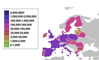
Figure 1. EU CO₂ emissions, in thousands of metric tons.

The goals of the surface response analysis for this problem are summarized below:

• starting from the second-order model derived in [3], we perform a canonical decomposition of the quadratic part of the model. This will provide for us the relevant combinations of attributable variables (the canonical variables), and their respective effect (increasing, decreasing, or neutral) on the CO₂ emissions;

• depending on the different types of contributions at second-order level, we will classify and compute the various types of confidence regions, for pairs of canonical variables. The classification will produce confidence regions of elliptical and hyperbolic types, whose specific geometric parameters we will compute;

• finally, we use the results of the analysis to make recommendations for optimal management of various attributable variables, both from the point of emission reductions, and from that of “cap-and-trade” policies, in order to optimize the energy and industry requirements of a state (or country) with respect to carbon emissions restrictions;

• the study concludes with a descriptive comparison between the relevant attributable variables in the case of EU and US. We observe that there are significant differences between the most relevant variables (both at the level of single-factor and as interactions), and discuss possible consequences of interest for future policy development.

2. The model, parameters, and descriptive quantities

We recall the final second-order model found in [3] to provide a good fit for the data and to have robust features for prediction and estimation:

$$[\widehat{CO}_{2}]^{-2.376} = 0.00000123+(710.85Fl-30.64Ga-3.4501Li)\times 10^{-13}+$$

$$+ (37.34Ga\cdot Bu+1.35Li\cdot Li-65.12Bu\cdot Bu-$$

$$- 133.05Li\cdot Fl-5.35Li\cdot Bu)\times 10^{-18}.$$

Throughout the paper, we will be using the the notation $x_{1}=$ Liquid Fuels (Li), $x_{2}=$ Gas Fuels (Ga), $x_{3}=$ Gas Flares (Fl), $x_{4}=$ Bunker (Bu) for the relevant attributable variables. With respect to these variables, the model becomes

(1) $$[\widehat{CO}_{2}]^{-2.376}=\beta_{0}+\sum_{i=1}^{4}\beta_{i}x_{i}+\sum_{i\leq j=1}^{4}\beta_{ij}x_{i}x_{j},$$

with the corresponding ranks determined by the stepwise SAS procedure are given in Table 1, along with the coefficients in the final regression model.

In matrix notation (where prime denotes transposition), (1) becomes

(2) $$Y=\beta_{0}+\beta^{\prime}\cdot X+X^{\prime}\cdot B\cdot X,$$

with the obvious identifications

$$X^{\prime}=(x_{1},\ldots,x_{4}),\,\,\beta^{\prime}=(\beta_{1},\ldots,\beta_{4}),\,\,B_{ij}=B_{ji}=\frac{1}{2}\beta_{ij}\,\,(i<j).$$

Table 1. Ranking by statistical relevance for attributable variables and interactions.

Rank	Variable	$\beta\left[\times 10^{-18}\right]$	$F-$ Value
$1$	Ga	$-30.635\times 10^{5}$	$197.22$
$2$	Ga:Bu	$37.3391$	$50.25$
$3$	Li:Li	$1.35565$	$47.74$
$4$	Bu:Bu	$-65.115$	$31.49$
$5$	Fl	$710.848\times 10^{5}$	$26.98$
$6$	Li:Fl	$-133.05$	$20.49$
$7$	Li:Bu	$-5.3501$	$19.07$
$8$	Li	$-3.4501\times 10^{5}$	$11.57$

More precisely, the vector $\beta$ (up to an overall scale factor of $10^{-13}$), and the symmetric matrix $B$ (up to an overall scale factor of $10^{-18}$) have the forms:

$$\beta=\left[\begin{array}[]{c}-3.4501\\ -30.635\\ 710.848\\ 0\end{array}\right],\,B=\left[\begin{array}[]{cccccc}2.7113&0&-133.05&0\\ 0&0&0&37.3391\\ -133.05&0&0&0\\ 0&37.3391&0&-130.23\\ \end{array}\right]$$

In order to perform the surface response analysis for this model, we must bring it to the simplest expression, by finding first its normal form and then its canonical decomposition. Since these operations require inverting the matrix of second-order interactions, we need to perform a preliminary calculation in order to determine its eigenvalues and corresponding orthonormal eigenvectors.

2.1. Eingenvalue analysis of the second-order interactions matrix

We recall that $\lambda_{k},V_{k}$ ($k=1,\ldots,4$) are the eigenvalues and normalized eigenvectors of the matrix $B$ if they solve the systems of linear equations:

$$B\cdot V_{k}=\lambda_{k}V_{k},\quad V^{\prime}_{k}\cdot V_{p}=\delta_{kp},$$

with $\delta_{ij}$ the Kronecker symbol, defined by $\delta_{ij}=1$ if $i=j$ and $\delta_{ij}=0$ otherwise. Then the matrix $B$ has the principal-value decomposition (c.f. [5, Appendix §C])

(3) $$B=\sum_{k=1}^{4}\lambda_{k}V_{k}V^{\prime}_{k}.$$

For the matrix $B$ found above, upon computing numerically the eigenvalues (using the SAS RSREG procedure [6] or Mathematica’s Eigensystem procedure), we arrive at

(4) $$\lambda_{1}=-140.176,\,\,\lambda_{2}=134.413,\,\,\lambda_{3}=-131.701,\,\,\lambda_{4}=9.94612,\,\,$$

up to the software numerical precision and the overall scale factor $10^{-18}$.

The four orthogonal and normalized eigenvectors are found to be

$$V_{1}=\left[\begin{array}[]{c}0\\ -0.257397\\ 0\\ 0.966306\end{array}\right],\,\,V_{2}=\left[\begin{array}[]{c}0.7107\\ 0\\ -0.703495\\ 0\end{array}\right],$$

$$V_{3}=\left[\begin{array}[]{c}-0.703495\\ 0\\ -0.7107\\ 0\end{array}\right],\,\,V_{4}=\left[\begin{array}[]{c}0\\ -0.966306\\ 0\\ -0.257397\end{array}\right].$$

2.2. Canonical analysis of the quadratic model

Let $B^{-1}$ represent the inverse of the matrix $B$ ([5, Appendix §C])

$$B^{-1}={\sum_{k=1}^{4}}\lambda_{k}^{-1}V_{k}V^{\prime}_{k},$$

and start from the model (2)

$$Y=\beta_{0}+\beta^{\prime}\cdot X+X^{\prime}\cdot B\cdot X.$$

In order to bring this expression to its normal form, we begin by shifting the variable $X$ by a constant term

$$\widehat{X}=X+\frac{1}{2}B^{-1}\cdot\beta.$$

Since $B$ is a non-singular matrix, we obtain the model

$${Y}=\beta_{0}+\beta^{\prime}\cdot\widehat{X}-\frac{1}{4}\beta^{\prime}\cdot B^{-1}\cdot\beta+\widehat{X}^{\prime}\cdot B\cdot\widehat{X}-\beta^{\prime}\cdot B\cdot B^{-1}\widehat{X},$$

where we have used the property $B^{-1}\cdot B=\mathbb{I}$. Therefore,

$${Y}=\beta_{0}-\frac{1}{4}\beta^{\prime}\cdot B^{-1}\cdot\beta+\widehat{X}^{\prime}\cdot B\cdot\widehat{X},$$

so we are now working with the normal quadratic form $\widehat{X}^{\prime}\cdot B\cdot\widehat{X}$. Using again (3), the quadratic form $\widehat{X}^{\prime}\cdot B\cdot\widehat{X}$ becomes

$$\widehat{X}^{\prime}\left(\sum_{k=1}^{4}\lambda_{k}V_{k}V^{\prime}_{k}\right)\widehat{X}=\sum_{k=1}^{4}\lambda_{k}(\widehat{X}^{\prime}V_{k})(V^{\prime}_{k}\widehat{X})=\sum_{k=1}^{4}\lambda_{k}|V^{\prime}_{k}\cdot\widehat{X}|^{2}=\sum_{k=1}^{4}\lambda_{k}z_{k}^{2},$$

where we have introduced the canonical coordinates

(5) $$z_{k}:=V^{\prime}_{k}\cdot\widehat{X},\quad k=1,2,3,4.$$

To conclude, we have the canonical form of the model

(6) $$Y-Y_{0}=(-140.176z_{1}^{2}+134.413z_{2}^{2}-131.701z_{3}^{2}+9.94612z_{4}^{2})\times 10^{-18},$$

with $z_{k}$ given in (5).

To find the stationary point of the model, defined generically as the zero-gradient point, we must solve simultaneously for all $k=1,\ldots,4$:

$$\frac{\partial Y}{\partial x_{k}}=0\Rightarrow\beta^{\prime}+2X^{\prime}\cdot B=0\Rightarrow B\cdot X=-\frac{1}{2}\beta,$$

which is equivalent to

$$B\cdot\widehat{X}=0\Rightarrow\widehat{X}=0,$$

because $B$ is non-degenerate. Together with (5), this gives the stationary point as the origin of the $z$ coordinates, $z_{1}=z_{2}=z_{3}=z_{4}=0$. In the original variables, the stationary point is found to be:

(7) $$X_{s}=-\frac{1}{2}B^{-1}\cdot\beta=\left[\begin{array}[]{c}-534271\\ -286155\\ -8294.32\\ -82045.4\end{array}\right],$$

up to an overall scale factor of $10^{5}$.

2.3. Confidence region shapes and conic sections

We repeat here the discussion regarding confidence region types presented in [2]. In order to distinguish between various types of shapes the confidence regions may have, we now specialize to a pair of variables $(z_{i},z_{j})$ from the normal quadratic form written in canonical variables, and impose the inequality

$$|Y-Y_{0}|\leq M,\quad M>0,$$

leading to

$$\Big{|}\lambda_{i}z_{i}^{2}+\lambda_{j}z_{j}^{2}\Big{|}\leq M,$$

which defines the confidence region centered at $(0,0)$. We find the following cases, corresponding to classes of conic sections:

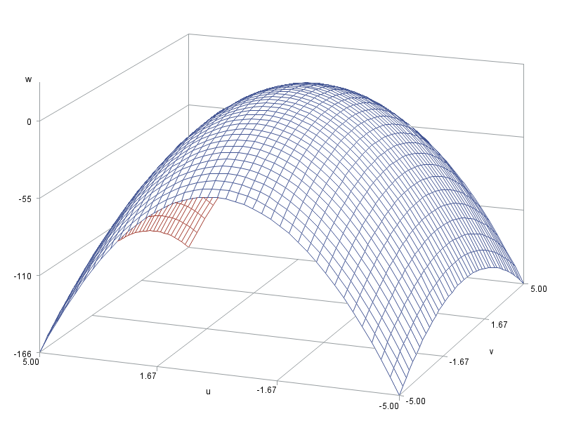
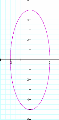
Figure 2. Confidence regions for the elliptical case.

2.3.1. Extremum point, elliptical region: all eigenvalues have the same sign

If $\lambda_{i,j}$ are either all positive or all negative, the point $(0,0)$ is a point of minimum or of maximum, respectively. The inequality becomes

(8) $$|\lambda_{i}|z_{i}^{2}+|\lambda_{j}|z_{j}^{2}\leq M\Rightarrow\frac{z_{i}^{2}}{M/|\lambda_{i}|}+\frac{z_{j}^{2}}{M/|\lambda_{j}|}\leq 1,$$

which defines the interior of an ellipse of semiaxes $\sqrt{M/|\lambda_{i}|},\sqrt{M/|\lambda_{j}|}$ (see Figure 2, right panel). The confidence region is given parametrically by:

(9) $$z_{i}=\sqrt{\frac{M}{|\lambda_{i}|}}r\cos(\theta),\quad z_{j}=\sqrt{\frac{M}{|\lambda_{j}|}}r\sin(\theta),\quad 0\leq r\leq 1,\,\,\theta\in[0,2\pi].$$

This is applicable for any pair of eigenvalues from $\{\lambda_{1},\lambda_{3}\}$ or from $\{\lambda_{2},\lambda_{4}\}$.

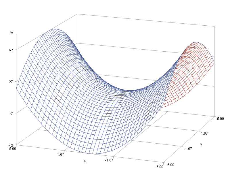
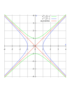
Figure 3. Confidence regions for the hyperbolic case.

Example 1.

Determining specific numerical regions for CO₂ fluctuations at levels discussed by IPCC [7].

In order to maintain consistency in comparing the models obtained for US [2] versus EU (this work), we compute the parameters of elliptical confidence regions for variables $z_{1},z_{3}$ and $z_{2},z_{4}$, corresponding to yearly CO₂ level fluctuations of 3% (see the discussion in [2, §4.1] and supporting documentation in [7]). As shown in [2, §4.1], this range of values corresponds to the order of magnitude $M\sim 10^{-8}$, so we arrive at the equations

(10) $$0.7107\widehat{X}_{1}-0.703495\widehat{X}_{3}=0,\quad-0.966306\widehat{X}_{2}-0.257397\widehat{X}_{4}=0,$$

(11) $$-0.257397\widehat{X}_{2}+0.966306\widehat{X}_{4}=8446.24\cdot r\cos(\theta),$$

(12) $$-0.703495\widehat{X}_{1}-0.7107\widehat{X}_{3}=8713.76\cdot r\sin(\theta),$$

which give the solution

(13) $$x_{1}=534271-6130.09\cdot r\sin(\theta),$$

(14) $$x_{2}=286155-2174.03\cdot r\cos(\theta),$$

(15) $$x_{3}=8294.32-6192.87\cdot r\sin(\theta),$$

(16) $$x_{4}=82045.4+8161.64\cdot r\cos(\theta),$$

where $0\leq r\leq 1,\theta\in[0,2\pi]$. It is important to note that this polar parametrization (in terms of the polar coordinates $r,\theta$) provides us with a confidence region more restrictive than just a product of maximal confidence intervals for individual variables $x_{1},x_{2},x_{3},x_{4}$. The maximal confidence intervals would simply be

(17) $$|x_{1}-534271|\leq 6130.09,\,\,|x_{2}-2286155|\leq 2174.03,$$

(18) $$|x_{3}-8294.32|\leq 6192.87,\,\,|x_{4}-82045.4|\leq 8161.64,$$

but the actual elliptical region will not include the set of minimal values $x_{1}=528141,x_{2}=283981,x_{3}=2101.45,x_{4}=73883.8$, for instance.

2.3.2. Saddle-point, hyperbolic region: non-zero eigenvalues of different signs

If, say, $\lambda_{i}>0$ and $\lambda_{j}<0$, then $(0,0)$ is a saddle point, and the inequality becomes

$$-M\leq|\lambda_{i}|z_{i}^{2}-|\lambda_{j}|z_{j}^{2}\leq M,$$

which defines the set of orthogonal hyperbolas (see Figure 3)

(19) $$\frac{z_{i}^{2}}{M/|\lambda_{i}|}-\frac{z_{j}^{2}}{M/|\lambda_{j}|}\leq 1,\quad\frac{z_{j}^{2}}{M/|\lambda_{j}|}-\frac{z_{i}^{2}}{M/|\lambda_{i}|}\leq 1.$$

The intersection of these conditions defines a region that looks like an elongated rectangle (elongated “corners”, the domain defined by the blue and green curves in Figure 3) and can be approximated with a rectangular shape. The confidence region is given parametrically by:

(20) $$z_{i}=\sqrt{\frac{M}{|\lambda_{i}|}}r\cosh(t),\quad z_{j}=\sqrt{\frac{M}{|\lambda_{j}|}}r\sinh(t),\quad-1\leq r\leq 1,\,\,t\in\mathbb{R}.$$

This would give confidence regions for any choice $\lambda_{i}\in\{\lambda_{1},\lambda_{3}\}$ and $\lambda_{j}\in\{\lambda_{2},\lambda_{4}\}$.

Example 2.

As before, we compute specific confidence regions corresponding to the IPCC recommended values for yearly CO₂ fluctuations.

Repeating the calculation performed in the previous example, for the case of hyperbolic confidence regions, we obtain (again, for $M\sim 10^{-8}$) the conditions

(21) $$x_{1}=534271-6130.08\cdot r\sinh(t),$$

(22) $$x_{2}=286155-2174.03\cdot r\cosh(t),$$

(23) $$x_{3}=8294.32-6067.93\cdot r\sinh(t),$$

(24) $$x_{4}=82045.4+8161.64\cdot r\cosh(t),$$

with $-1\leq r\leq 1,t\in\mathbb{R}$.

Notice that this does not provide an actual confidence region (the domain defined is unbounded), consistent with the geometric features shown in Figure 3.

However, we can extract from the conditions above specific linear relationships between the variables that can be used for comparison purposes. Such linear relationships (which correspond to the asymptotic lines shown in Figure 3, second panel) can be used to find equivalencies between variables $x_{1},x_{3}$ and $x_{2},x_{4}$. We perform this numerical analysis in Section 3.2, and indicate how to interpret the results.

3. Conclusions and predictions based on nonlinear analysis

Throughout this subsection, we let the values of the attributable variables $X^{\prime}=(x_{1},x_{2},x_{3},x_{4})$ be measured from the stationary point $X_{s}=-\frac{1}{2}B^{-1}\cdot\beta$ (7).

3.1. Nonlinear analysis of contributing factors

Starting from (6)

$$Y-Y_{0}=(-140.176z_{1}^{2}+134.413z_{2}^{2}-131.701z_{3}^{2}+9.94612z_{4}^{2})\times 10^{-18},$$

and the power-law transformation

$$Y=({\mbox{CO}}_{2})^{-2.376},$$

we first make the important remark that increasing/decreasing CO₂ is equivalent to decreasing/increasing $Y$.

Next, using the defining relations for the linear combinations $z_{k}=V^{\prime}_{k}\cdot\widehat{X}$, with $V_{k}$ given in §2.1, we notice that the combinations $z_{1},z_{3}$ contribute to increase the CO₂ emissions via interactions, while $z_{2},z_{4}$ actually decrease it. Given that (measured from the stationary point $X_{s}$),

$$z_{1}=-0.257397Ga+0.966306Bu,\quad z_{2}=0.7107Li-0.703495Fl,$$

$$z_{3}=-0.703495Li-0.7107Fl,\quad z_{4}=-0.966306Ga-0.257397Bu,$$

we notice that $z_{1}$, which is mostly a combination of Gas Fuels and Bunker, has the most damaging effect. Along with the fact that $x_{1}$ (Gas Fuels) ranks first among significant attributables in the second-order model, we can conclude that Gas-related sources seem to be the most significant factors responsible to the atmospheric CO₂ for the European countries studied here.

3.2. Relative importance of attributable variables

Finally, we can estimate the correct combinations between attributable variables $x_{1}-x_{4}$ which would keep the CO₂ level constant, based on our model. It is particularly useful to observe that the variables $z_{1},z_{4}$ are linear combinations only of attributables Ga, Bu, while $z_{2},z_{3}$ are derived from the attributables Li, Fl. Therefore, it is natural to impose the conditions

$$\lambda_{2}z_{2}^{2}-|\lambda|_{3}z_{3}^{2}=0,\quad-|\lambda_{1}|z_{1}^{2}+\lambda_{4}z_{4}^{2}=0,$$

from which we obtain the hyperplane equations

$$z_{1}=\pm\sqrt{\left|\frac{\lambda_{4}}{\lambda_{1}}\right|}z_{4},\quad z_{2}=\pm\sqrt{\left|\frac{\lambda_{3}}{\lambda_{2}}\right|}z_{3}.$$

These equations (using §2.1) lead to the linear relationships between Ga-Bu and Li-Fl given below:

$$-0.257397Ga+0.966306Bu=\pm 0.266372913(-0.966306Ga-0.257397Bu)$$

$$0.7107Li-0.703495Fl=\pm 0.989860283(-0.703495Li-0.7107Fl).$$

From these equations it is possible to develop an equivalence between different attributables, and to use such identities in order to develop policy and accountability criteria. The only acceptable solutions (selected by positivity of proportionality coefficients) yield:

(25) $$Ga=1.74388Bu,\quad Li=98.1284Fl.$$

In other words, under a “CO₂ trade” policy developed under these guidelines, one unit of Gas fuel is equivalent to 1.74388 unit of Bunker, while one unit of Liquid Fuel can be replaced by 98.1284 units of Gas Flares. It is important to note that this “conversion formula” corresponds to the condition $M=0$, i.e. no variation in the CO₂ levels. For any other value of $M$, the formulas would provide different conversion values, as we show below.

3.3. Comparing the US and EU models

Using the results obtained in [2], it is possible develop a comparison between the US and EU quadratic models for attributable variables and interactions; in particular, it is possible to compare the relative relevance of the main single-factor variables and of the main interactions (see Table 2).

Table 2. Comparison of statistical relevance for attributable variables and interactions, US vs. EU.

Rank	Variable in US	Variable in EU
$1$	Liquid	Gas
$2$	Liquid:Cement	Gas:Bunker
$3$	Cement:Bunker	Liquid:Liquid
$4$	Bunker	Bunker:Bunker
$5$	Cement	Gas Flares
$6$	Gas Flares	Liquid:Gas Flares
$7$	Gas	Liquid:Bunker
$8$	Gas:Gas Flares	Liquid

In order to complete the comparison between the US and EU models, initiated in [2], we evaluate conversion rates between attributable variables, corresponding to the same range of CO₂ level fluctuations as mandated by the IPCC ($M\sim 10^{-8}$ as shown in [2, §4.1]). As mentioned above, for a given value of $M\neq 0$, the conversion rates found earlier (for $M=0$) are not valid anymore. Instead, we start from the relations (21)-(24) (derived specifically for $M\sim 10^{-8}$), and arrive at the linear relations established from these models:

(26) $$\frac{x_{1}-534271}{6130.08}=\frac{x_{3}-8294.32}{6067.93}=r\sinh(t),$$

(27) $$-\frac{x_{2}-286155}{2174.03}=\frac{x_{4}-82045.4}{8161.64}=r\cosh(t).$$

Therefore, we conclude that under these conditions, one unit variation of $x_{1}$ (Liquid) corresponds to $6130.08/6067.93\simeq 1.01$ units variations of $x_{3}$ (Gas Flares). Recall that in the US study [2] we concluded that 1000 units of Gas Flares can be equated to 2127 units of Cement; the current study shows that in the case of EU, one unit of Liquid is equivalent to approximately 1.01 units of Gas Flares. However, a direct comparison of the various trading values cannot be derived, which is yet another indication that such studies must be performed regionally, and that application of uniform policies is not supported by the data.

References

- [1] Yong Xu and Chris Tsokos (2013), Attributable variables with interactions that contribute to CO2 in the atmosphere, Frontiers in Science, 3(1): 6-13.
- [2] Chris Tsokos and Iuliana Teodorescu (2013), Surface response analysis and determination of confidence regions, preprint.
- [3] Chris Tsokos and Iuliana Teodorescu (2013), Contributors of carbon dioxide in the atmosphere in Europe, preprint.
- [4] http:en.wikipedia.org/wiki/File:Countries by carbon dioxide emissions world maps deobfuscated.png
- [5] Ronald Christensen (2011), Plane answers to complex questions, Springer Texts in Statistics.
- [6] Online documentation for SAS: [http://support.sas.com/documentation/cdl/en /statug/63033/HTML/default/viewer.htm#rsreg-toc.htm]
- [7] Intergovernmental Panel on Climate Change reports: [http://www.ipcc-data.org/ddc co2.html]; [http://www.ipcc.ch/pdf/assessment-report/ar4/wg3/ar4-wg3-chapter13. pdf]