Combined field formulation and a simple stable explicit interface advancing scheme for fluid structure interaction
Abstract
We develop a combined field formulation for the fluid structure (FS) interaction problem. The unknowns are , being the fluid velocity, fluid pressure and solid velocity. This combined field formulation uses Arbitrary Lagrangian Eulerian (ALE) description for the fluid and Lagrangian description for the solid. It automatically enforces the simultaneous continuities of both velocity and traction along the FS interface. We present a first order in time fully discrete scheme when the flow is incompressible Navier-Stokes and when the solid is elastic. The interface position is determined by first order extrapolation so that the generation of the fluid mesh and the computation of are decoupled. This explicit interface advancing enables us to save half of the unknowns comparing with traditional monolithic schemes. When the solid has convex strain energy (e.g. linear elastic), we prove that the total energy of the fluid and the solid at time is bounded by the total energy at time . Like in the continuous case, the fluid mesh velocity which is used in ALE description does not enter into the stability bound. Surprisingly, the nonlinear convection term in the Navier-Stokes equations plays a crucial role to stabilize the scheme and the stability result does not apply to Stokes flow. As the nonlinear convection term is treated semi-implicitly, in each time step, we only need to solve a linear system (and only once) which involves merely if the solid is linear elastic. Two numerical tests including the benchmark test of Navier-Stokes flow past a Saint Venant-Kirchhoff elastic bar are performed. In addition to the stability, we also confirm the first order temporal accuracy of our explicit interface advancing scheme.
keywords:
Fluid Structure Interaction; Arbitrary Lagrangian Eulerian; Navier-Stokes Equations; Saint Venant-Kirchhoff;1 Introduction
The interaction of a rigid or deformable solid with its surrounding fluid or the fluid it enclosed gives rise to a very rich variety of phenomena. For example, a rotating fan, a vibrating aircraft wing, a swimming fish. The daily activities of many parts of our human body are also intimately related to this fluid solid or more commonly called fluid structure (FS) interaction. For example, the heart beating, respiration, speaking, hearing, and even snoring. To understand those phenomena, we need to model both the fluid and the solid. In this paper, we assume the fluid is incompressible and the solid is deformable. The governing equations for FS interaction are then as follows:
| (1.1) | |||
| (1.2) |
In the above equations, is the fluid domain at time and is the initial configuration of the solid. is the velocity at a spatial point in . is the position at time of a material point in . Constants and are the densities of the fluid and the solid. As one can tell, the fluid is described by the Eulerian (spatial) description while the solid is described by the Lagrangian (material) description with reference configuration . is the stress of the fluid in the Eulerian description and is the stress of the solid in the Lagrangian description. If the fluid is assumed to be viscous Newtonian,
| (1.3) |
If the solid is elastic, then there is a strain energy with density :
| (1.4) |
so that the stress is determined by . Here is the deformation gradient. As a result, satisfies
| (1.5) |
Like in , we write instead of for simplicity. Here and . Let be the strain tensor. If the strain of the solid is small, we can model the solid as Saint Venant-Kirchhoff material with . Simple calculation shows
| (1.6) |
If the deformation of the solid is small, one popular choice of is
| (1.7) |
where is the displacement vector. We can define an associated with and check . We can also verify the convexity of :
But we will see later that is not convex (see (3.40)). Indeed, it is not even polyconvex [9, sec 3.9]
The fluid and the solid are coupled by the continuity of velocity and traction across the FS interface. Mathematically, it can be written as (see Antman [1, p.485, , p.489, (15.31)])
| (1.8) | |||
| (1.9) |
Here is the FS interface at and is any part of it. is the image of at time under the mapping and it is part of the fluid boundary. and are the outward normals. Besides the interface conditions (1.8) and (1.9), we also need boundary conditions on the rest of the boundaries. These fixed boundaries are called to : , . We require
| (1.10) |
Here , , and are prescribed fluid velocity, fluid traction, solid position and solid traction on the ’s.
The well-posedness of FS interaction problems has been studied for various models (see [11, 16, 10] and the references in [10]). When the solid is deformable, the analysis uses Lagrangian description for both the fluid and the solid [16, 10]. But for computational efficiency, we use Arbitrary Lagrangian Eulerian (ALE) description for fluid in this paper. We learn from [14] the idea of using conservative ALE description with proper intermediate mesh or meshes so that the stability bound obtained does not explicitly depend on the mesh movement. But [14] only considers the convection diffusion equation on a domain whose motion is known.
We will show that (1.9) is equivalent to (2.18) while the latter is more popular in the literature. Schemes based on {(1.1),(1.2),(1.8), (2.18), (1.10)} can be classified into two classes: partitioned schemes and monolithic schemes. In a partitioned scheme ([5, 12]), different solvers are used for fluid and elastic equations. For stability reason, one may hope that the two interface conditions (1.8) and (2.18) are satisfied simultaneously. But this cannot be achieved with one single iteration between the fluid and the solid solvers. Various improvements have been proposed: [13, 2] reduce the fluid-structure coupling to pressure-structure coupling after a temporal discretization; [17] proposes a beautiful stable splitting scheme for fluid-membrane interaction problem; [15] discusses how to achieve fast convergence by properly choosing the boundary conditions for different solvers. So far, all the numerical analysis requires that the fluid domain does not move and the flow is Stokes type [13, 17, 15]. These assumptions conceal the important fact that the convection term in the Navier-Stokes equations indeed stabilizes the scheme when the domain moves. In a monolithic scheme ([18, 4]), the governing equations for the fluid and the solid as well as the governing equation for the displacement of the mesh are coupled and solved all together. Hence a large nonlinear system is required to solve in each time step [4, remark below (3.11)] [18, section 3.5]. Since the interface conditions (1.8) and (2.18) are built into the system, they are automatically satisfied once the system is solved. Then it is easy to believe that monolithic schemes will preserve the stability of the associated continuous models. However, as the discrete schemes so far proposed are very complicated, we are not aware of any proof of existence and stability of numerical solutions in the literature.
The celebrated immersed boundary method of Peskin [25] uses delta function to represent the force at the FS interface. When the solid is codimension-1, i.e., a surface in or a curve in , there comes the immersed interface method of LeVeque and Li [19] which is spatially more accurate. In this method, instead of using delta function, the forces are translated into the jump conditions across the interface. These jump conditions are then taken care by changing the discretization of the differential operators at stencils acrossing the interface [19, 3]. To our point of view, there are still some aspects left to be improved for the methods initiated by Peskin, LeVeque and Li: Immersed boundary method in general is only first order in space [25, p.500,p.509], [3, p.4]; Immersed interface method cannot handle solid with a finite volume.
In this paper, we will present a new monolithic scheme. It is based on a new formulation of FS interaction which in some aspect is similar to the well-known one field formulation of multi-fluid flows (see [29, (1)] for example, but you will not see any delta function in our method). In our scheme, the unknown is , being the fluid velocity, fluid pressure and solid velocity. There are many nice features of our scheme:
-
1)
(Explicit mesh moving) Our scheme is explicit interface advancing which means that the FS interface at time is constructed explicitly using only information of the solid at time . So, determining the FS interface and computing are decoupled.
-
2)
(Smaller system) Let be the fluid velocity. Let and be the solid velocity and position. Let and be the fluid mesh velocity and position. Then, ignoring the pressure for simplicity, [18, (37)]’s unknown is , and [4, (3.10)]’s unknown is . Our unknown is . In our scheme, the mesh related information and the solid position are all treated explicitly.
- 3)
-
4)
(Easy implementation) As our scheme is Jacobian free and does not require characteristics, it is very easy to implement.
-
5)
(Stability) The most important feature of our scheme is its stability: Even though the fluid mesh is constructed explicitly, the total energy of the fluid and the solid at time is bounded by the total energy at time . The stability bound hence obtained does not explicitly depend on the fluid mesh velocity which however is explicitly used in the computation through the ALE formulation (see Theorem 10 which is our main theorem). This feature is shared by the original continuous model (see Theorem 4). Surprisingly, the nonlinear convection term in the Navier-Stokes equations plays a crucial role in proving Theorem 10 and the stability result does not apply to Stokes flow.
However, as the energy bound alone at is not enough to prevent the FS interface from colliding with itself or other fixed boundaries at , we have to assume (but see Remark 4.1) that the we take satisfies the following collision free condition so that we are able to construct the fluid mesh at time :
| (1.11) |
As the interface is determined by extrapolation, one may wonder what is the point to use a monolithic scheme — can the unknowns be easily solved for separately? If one try that, the scheme becomes a loosely coupled partitioned scheme. Consequently, there will be time lag in the enforcement of the two continuity conditions. How this time lag affects the stability will not be addressed in this paper and we refer to [5, 12] and the references therein. By paying the price of solving a larger system, monolithic scheme enables the satisfaction both (1.8) and (2.18) at the same time which is the key to get stability in all density ratio regime. How to solve the system for efficiently will not be addressed in this paper, even though we do have a linear system when it is Navier-Stokes and linear elasticity coupling.
As extrapolation is used to determine the interface position, one may wonder whether it will damage the accuracy. We note that the position of any point satisfies where is the solid velocity. We know using the right end point rule (hence implicit) to approximate the integral is not necessarily more accurate than using the left end point rule (hence explicit). Obviously, left end point rule is cheaper. Less obviously, as we have mentioned and will prove later, left end point rule is also stable if it is handled properly. We will present numerical test that verifies the first order temporal accuracy in Section 5 (see Table 2 and Fig. 3). Higher order schemes will be discussed in a forthcoming paper.
The rest of the paper is organized as follows: In Section 2 we introduce the combined field formulation and its weak form for FS interaction, and also discuss the conservative ALE description of it. We present our scheme in Section 3, starting from the discretization of the solid part. Then we discuss the fluid mesh construction, the ALE mapping and its applications. In particular, we can define the backward in time ( ) and the forward in time () extension (see (3.52) and (3.63)). Before we introduce our scheme (3.68), we mention two results (Lemma 7 and Corollary 8) which are related to Geometric Conservation Law and present Lemma 9 which contributes to some crucial cancelation that will be used in the stability proof. After this long preparation, we prove the stability of our scheme in Section 4. This is our main theoretical result (Theorem 10). Two numerical tests will be discussed in Section 5. They verfies the stability as well as the first order temporal accuracy of our scheme.
2 Combined field formulation using ALE description
We show that the FS system {(1.1),(1.2),(1.8),(1.9),(1.10)} has a very clean and simple weak formulation. Then we put it into ALE format using the conservative formulation. To save space, we will not discuss the non-conservative formulation but refer the readers to [21].
2.1 Traction boundary condition
We first show that we can insert test functions into the traction boundary condition (1.9) ([1, page 489]).
Lemma 1.
Let be the FS interface at . If (1.9) is true, then for any and any that is defined on ,
| (2.12) |
where is defined on and satisfies .
Proof.
Consider . Suppose is the image of the mapping with . Then, when , the mapping maps to and then to . So, we can change all the integrations to :
| (2.13) |
| (2.14) |
With the same idea, (1.9) can be rewritten as
| (2.15) |
As the above equation is true for any , the integrand must be zero. Then, since , we get
| (2.16) |
Now, putting (2.13),(2.14),(2.16) together, we obtain (2.12). ∎
2.2 Combined field formulation
We will use velocity field as the unknown for both fluid and solid because it leads to a simple enforcement of the boundary condition (1.8). The combined field formulation for time dependent FS interaction is as follows:
| (2.19) | |||
| (2.20) | |||
| (2.21) | |||
| (2.22) | |||
| (2.23) |
where is defined by through for any . is the FS interface at . . and are fixed boundaries. At the initial time , we are given , and being the initial fluid velocity, initial solid velocity and initial solid position.
Now we will derive a weak form of (2.19)–(2.23). Suppose we know a function defined on , introduce
| (2.24) |
Note that and are defined on different domains (see Fig. 1 for an illustration). is given from the very beginning and will never change. is varying with respect to . We require since can be rather nonlinear. But for linear elasticity (1.7), requiring is enough.
Theorem 2.
Proof.
The boundary condition (2.21) has been built into the function space . We dot (2.19a) with , dot (2.19b) with and dot (2.20) with . After integration by parts for the and terms, we add the resulting equations together. The boundary integrals on and cancel each other because of (2.22) and the definition of . ∎
2.3 Stability identity for (2.25)
We want to derive some stability identity for (2.25) when the solid has a strain energy (1.4). Once again, we denote by . With the defined in (1.4),
| (2.26) |
We have the following identity for divergence free velocity field which can be applied to the first term in (2.25) when and :
Lemma 3.
Consider a divergence free velocity field defined on a time varying domain . Assume at any point on , either or where is the outward normal and is the velocity that moves. Then
| (2.27) |
Proof.
Recall the following Reynolds transport theorem ([1, page 488, (15.23)]): for any ,
| (2.28) |
So,
| (2.29) |
In the last step we have used the condition either or on . Using the divergence free condition, the last surface integral can be rewritten as
| (2.30) |
We have used in the last step. Plugging (2.30) into (2.29), we get (2.27). ∎
2.4 Conservative formulation of Arbitrary Lagrangian Eulerian (ALE) description
When the time reaches (which can be any number), we choose the as the reference domain and construct a backward in time mapping that maps to for any . See (3.47) for a way of constructing . Note that . Define
| (2.32) |
With this fixed, we set in (2.25) and choose test function satisfing
| (2.33) |
In a finite element method, requiring (2.33) for a basis function means the function is always attached to the nodal point it starts from no matter how the mesh moves. See (3.52),(3.53). Evaluating (2.33) at and using , we obtain
| (2.34) |
As is exactly the velocity of domain , we can apply the Reynolds transport theorem (2.28) with to get
| (2.35) |
where the integrand on the right hand side is evaluated at . Because of (2.34), the sum of the last two terms in the integrand equals . So, using , (2.35) leads to
| (2.36) |
To summarize, if with , is a solution to (2.19)–(2.23), then satisfies the following: For any , for any given backward in time mapping , for any defined in the space-time domain of the fluid, and satisfying and , for any defined in and satisfying and ,
| (2.37) |
3 Fully discrete scheme
Now we turn to the fully discrete scheme. The initial set up is as follows: First of all, there is a mesh for the solid reference domain . Part of the boundary grid points of form a mesh for . Suppose we are given , , and suppose we also have the mesh of domain where is our numerical approximation for the fluid domain at time . Without loss of generality, we use elements for fluid velocity, fluid pressure and solid velocity. For efficiency and also to meet the requirement of optimal isoparametric finite element mesh, we require that an edge of (or ) is straight when it does not belong to the boundary of (or ) and is curved otherwise. Here edge refers to both surface and edge if .
3.1 Solid part
The first order in time discretization for the solid part (3rd line in (2.37)) is rather simple. So we discuss it first. Recall at time , we have and on . For the next moment , define
| (3.38) |
Through out this paper, is always constructed explicitly in this way. To determine , we have two different approaches:
3.1.1 Efficient semi-implicit discretization for nonlinear material
When , we have:
| (3.39) |
where . The exact formulas for the variational derivatives of various materials should be widely available in the literature as they are used to derive the Newton’s method for solving . For Saint Venant-Kirchhoff material (1.6),
| (3.40) |
where and . is a bilinear functional of and . Of course, if we use linear constitutive equation (1.7), the approximately equal sign in (3.39) becomes the equal sign.
3.1.2 Stable implicit discretization for material with convex strain energy
The above semi-implicit discretization is what we will use in our numerical test. But to prove unconditional stability for more general nonlinear elastic solid, we need to consider fully implicit discretization. The existence of the solution will be address in a later section (Section 4.1) after we also include the fluid variables.
3.1.3 Special case
3.2 Fluid part
Now, let us move to the fluid part in (2.25). One nice feature of our scheme is that we use explicit interface advancing. This makes our scheme very efficient, provided that it will not damage the accuracy (Table 2 and Fig 3) and the stability (Theorem 10).
So, we define by (3.38) which is an explicit extrapolation. From the values of at the grid points of , we determine the numerical FS interface at time . Moveover, from those values and also the information from fixed boundaries and , we are able to determine all the boundary grid points of . In particular, we know the position of all boundary vertices of . Using the latter as boundary value, we use (not !) element to solve a linear anisotropic elasticity equation on . We use for each triangle . The idea of increasing the stiffness of small elements to prevent them from being distorted comes from [23]. The result gives positions of vertices of all the triangles of . We always used to construct so that we do not have to reconstruct the stiffness matrix in each time step. Certainly more sophisticated method can be used, but we shall not discuss those alternatives.
Recall that we use elements. To guarantee optimal rate of approximation on an isoparametric finite element mesh, all its interior triangles should be straight and are standard Lagrange elements. But specific placement of interior grid points on curved triangles is mandatory [26, 8, 20]. So, once we have all the vertices and boundary grid points of , we can determine all the grid points except which denotes grid points lying inside a curved triangle touching the boundary. When , we are done as . When , we need [26, 20]. We use Scott’s procedure [26] when . Consequently, is uniquely determined by grid points on the boundary edges (due to the mapping and the prefactor in [20, (14)]). When , we need to construct some local chart before we can use [20, (22)] to determine .
3.2.1 The mapping in the ALE description
To construct , the basic idea is to use the fact that any physical triangle ,
no matter which time level it is at, is mapped to the same reference triangle with vertices
,,…,
.
We use to denote this mapping
where denotes the th triangle of .
Then is defined piecewisely on each triangle
as follows:
| (3.47) |
Here and maps to . Note that and maps to . The explicit formula of is well-known [8]:
| (3.48) |
Here is the number of grid points on each triangle. is the scalar finite element basis function on . is the local index. are the th grid point of . is the global index. is the mapping from local index to global index on the th triangle. Using these notations, we have the following result
Lemma 5.
The defined by (3.47) satisfies
| (3.49) |
where is the scalar finite element basis function on that is associated with the th grid point and is the total number of grid points. Consequently, and
| (3.50) |
are in the finite element space on .
3.2.2 Intermediate fluid meshes
In the conservative ALE scheme, we need intermediate fluid domains that lie between and . Their constructions make use of the defined in (3.47). For , define
| (3.51) |
Note that maps all the grid points of to which then form a mesh. We called this mesh . As is reduced to affine linear mapping when is a straight triangle, it is easy to see that all the interior triangles of are straight.
3.2.3 Backward in time extension
Recall that on , we use to denote the scalar basis function associated with the th grid point. Define its backward in time extension
| (3.52) |
for . An immediate consequence is that for any . Hence
| (3.53) |
3.2.4 Related properties
As is a finite element mesh by itself, for any triangle , automatically there is a mapping that maps to . Like (3.48), this is given by where is the th grid point of and its global index is . Because of (3.49) and the way we construct , we know . On the other hand, the mapping also maps to . By (3.47), we have
| (3.54) |
So we see that is exactly . As a result of (3.54), we get if . Consequently, we have the following nice property for numerical implementation.
Proposition 6.
The backward in time extension which is defined by (3.52) is nothing but the standard basis function associated with the th grid point on for any .
Proof.
If is in the finite element space on , it has an expansion with being the number of grid points on . Here, and the vector scalar product . We can define the backward in time extension of as follows:
| (3.56) |
In particular, recalling that the defined in (3.50) is in the finite element space on , we have . Its backward in time extension in the space-time domain is defined as
| (3.57) |
With ready, we can study the relation between for and . This is the key to understand the Geometric Conservation Law.
Lemma 7.
Let be any function on and let be its backward in time extension defined by (3.52). When ,
| (3.58) |
where the divergence in is taken with respect to the variable. Note that the first integrand equals to . If the right hand side of (3.58) should be
| (3.59) |
with and being the two quadrature points of the two-point Gauss quadrature on .
Proof.
The following argument is essentially the proof of Reynolds transport theorem (2.28) (see [1, p.487]). To simplify the notation, we write as .
In the second step, we have changed variables and in the last step we have used (3.53). Note that as is independent of , the integrand in the last expression is a polynomial of degree in where is the spatial dimension. To integrate it exactly, when , we can use the mid-point rule and when we can use Gauss quadrature. Take as an example: The right hand side of the above equation equals
| (3.60) |
Now, let and recall .
| (3.61) |
Then, because of (3.57), . Hence
So we can continue (3.61) and obtain
Putting all together, we have
After a change of variable and using (3.51), we obtain (3.58). ∎
Because in the above proof we only use , the in (3.58) can be changed to . Therefore, we have the following Corollary:
Corollary 8.
When , we have
| (3.62) |
where is any function defined on and is its backward in time extension . Using Gauss quadrature in time, we have similar formula when .
Now we study the relation between the mesh velocity and fluid velocity . Note that is defined on while is defined on . But by Proposition 6, . So, we can introduce the forward in time extension defined in the space-time domain :
| (3.63) |
Lemma 9.
Note that is the FS interface. For any ,
| (3.64) |
Proof.
From (3.49) and (3.50), we know . Hence . Comparing it with (3.63), we are left to show that if is the index of a grid point on the FS interface.
In the later discussion (see the very last condition in the definition of in (3.67)), we will see that fluid velocity and solid velocity agree at the grid points on the FS interface.
Let us use to denote grid points on for . So, by the way we construct (recall ), we know moves to , i.e., . Therefore . ∎
3.3 The complete scheme
From now on, we use the notation
| (3.65) | |||
| (3.66) |
Inspired by (2.37), we propose the following first order scheme: Suppose we are given , , and . For the next moment , first define by (3.38):
Next, we construct and then the intermediate mesh following the discussion in the beginning of Section 3.2 and then Section 3.2.2. Then we explicitly construct mesh velocity using (3.50) which is a finite element function defined on . Define the Lagrange finite element space as follows:
| (3.67) |
Here is the mesh of . and are the meshes of and respectively. is the mapping from the reference triangle to the th physical triangle of the fluid domain at time which is denoted by . is defined similarly, but for triangle .
Now, find with and so that for any finite element triple with and ,
| (3.68) |
The in (3.68) is the backward in time extension of vector basis function by (3.52) (with obvious extension to vectors). is the backward in time extension of by (3.56). is the forward in time extension of by (3.63). The technique of adding the term containing is standard and is initiated by [27]. The above scheme is for . When , the 2nd and the 3rd lines of (3.68) should be changed to
| (3.69) |
where forms the two-point Gauss quadrature on (Lemma 7).
Let , and . (3.68) leads to a system of equations for and is linear for the fluid variables. Proposition 6 tells us that the assembling of the load vectors and various matrices for each term in (3.68) uses only standard finite element basis functions defined on the corresponding mesh indicated by the subscripts , or respectively.
Lastly, we would like to stress that the last equality condition in the definition of ((3.67)) is trivial to enforce and will not complicate the programming: When assembling the matrices and vectors, we simply need to equate the global index of the fluid basis function that is associated with with the global index of the solid basis function that is associated with , for all grid point .
4 Stability
Now, we are ready to prove the stability of scheme (3.68).
Theorem 10.
Proof.
We have discussed the solid part (5th line in (3.68)) in Section 3.1.2 which leads to (3.45). In (3.68), let , and . Note that becomes . We obtain
| (4.71) |
Here, without loss of generality we consider . Now, look at the 2nd line in the above inequality and recall . After integration by part, we find it equals
Integration by part once again, the 2nd line in (4.71) becomes
| (4.72) |
Because of the assumption and and Lemma 9 (indeed, we only need their normal components equal), the boundary integral in (4.72) vanishes. The first half of the volume integral in (4.72) cancels with the 3rd line of (4.71). So, (4.71) now becomes
| (4.73) |
Then we make use of (3.62) to handle the 2nd and the 5th terms. Finally, we use to conclude. ∎
Remark 4.1.
Our FSI solver works as follows: at , we have , , . First, we define . Then we assume (1.11) is satisfied so that we can construct the fluid domain with mesh . Then, on and , we solve for . Immediately there comes a good news for the construction of which is for the next step: From (4.70), even at , we already know
| (4.74) |
For simplicity, we have assumed linear elasticity with and ignored the body forces and . So is rather regular which makes the assumption (1.11) less stringent because the construction of uses . Obviously, larger and would provide larger support for validating assumption (1.11). When , our method solves fluid and rigid body interaction problem.
4.1 Existence and uniqueness
Certainly, before we ever discuss the stability, we need show the system (3.68) does have a solution. As the mesh is determined explicitly and the convection term in the fluid is handled semi-implicitly, the only nonlinear term is .
If the solid is linear elastic (see (1.7)), (3.68) is indeed a linear system for and existence follows. The uniqueness follows from the stability results: When all the forcing terms vanish, by choosing , we know and . Then (3.68) implies for all in the finite element space for fluid velocity and having zero boundary condition on . So, by the inf-sup condition, .
For nonlinear solid with convex strain energy, we need to assume , and . Then the stability itself will imply existence by the following Lemma [27, Chap 2. Lemma 1.4]. The proof is a simple application of Brouwer fixed point theorem.
Lemma 11.
Let be a finite dimensional Hilbert space with inner product and norm . Let T be a continuous mapping from into itself such that there is a constant so that
Then there exists with such that .
Proof.
It is clear that we can define a continuous mapping as well as the space and inner product so that (3.68) can be written as
The subscript in means the mapping depends on and also boundary data and body forces. From (4.70), we know which is positive when is large enough. Hence the existence follows from Lemma 11.
Now consider the uniqueness. Because of the convexity of and ,
| (4.75) |
for any and . Now suppose we have two solution of (3.68). Let us call them and . We take difference of the (3.68)’s satisfied by and respectively and let the test function be . From the stability results as well as (4.75), we immediately obtain and . After that, from the difference of the (3.68)’s, we have
for all in the finite element space for fluid velocity and having zero boundary condition on . So, by the inf-sup condition, . ∎
5 Numerical test
The finite element package we have implemented is in some sense an upgraded version of iFEM due to Long Chen [6, 7]. iFEM is an adaptive piecewise linear finite element package based on MATLAB. It uses a beautiful data structure to represent the mesh and also provides efficient MATLAB subroutines to manipulate the mesh. In particular, local refinement and coarsening can be done fairly easily. For our purposes, we have extended it to Taylor-Hood isoparametric Lagrange elements with . The finite element mesh is generated by the DistMesh of Persson and Strang [24].
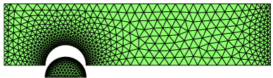
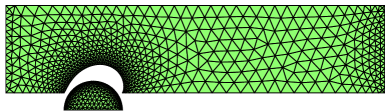
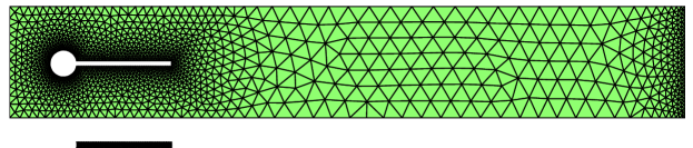
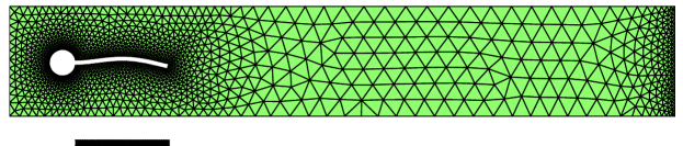
We present two numerical tests: (I) The first case is Navier-Stokes flow past a linear elastic semi-cylinder. See Fig. 1 for an illustration. The semi-cylinder is placed inside a channel and is attached to the floor. The size of the channel is . The cylinder is centered at and has radius 0.5. The inflow from the left is prescribed by where when and when . At the outflow boundary, we use as the boundary condition [22]. (II) The second case is a Navier-Stokes flow enforced vibrating bar. This problem is proposed by [28]. See Fig. 4 for an illustration. A rigid cylinder centered at with radius is fixed inside a channel of size . A horizontal St. Venant-Kirchhoff bar with length 0.35 and width 0.02 is attached to the rigid cylinder. The surface where they touch is curved. The center of the cylinder and the center of the bar have the same height initially. The material point on the tail of the bar which is initially at is called . The inflow velocity of the channel is where the same as in case (I) is used. We also use the same outflow boundary condition as in case (I). The physical parameters for these two test problems are listed in Table 1.
| solid type | ||||||||
| case (I) | linear | 1 | 1 | 1 | 50 | 500 | (0,0) | (0,0) |
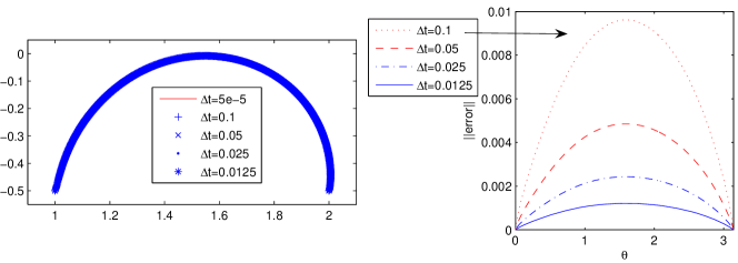
| case (II) | St.Venant-Kirchhoff | 1 | 0.001 | 1 | 2000 | 8000 | (0,) | (0,) |
The scheme we tested is (3.68) except that the St. Venant-Kirchhoff material in case (II) is treated semi-implicitly by (3.41) for efficiency.
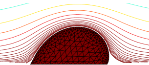
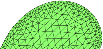
We use case (I) for both stability and accuracy check. To verify the stability, we use elements and take to integrate to . The computational mesh is shown in Fig. 1. In the captions, we state parameters of the meshes where and are the sizes of the largest and smallest edges. The computational domain for the fluid will change but the computational domain for the solid will remain the same. When , by (so after 4 iterations if doing time matching), the system has almost reached steady state. The CPU time in that situation is about 12 seconds on an IBM Thinkpad laptop with 3G memory. Even though it has intel Core 2 Duo CPU @ 2.8 GHz, the Matlab is run on a single thread mode. We compare our result with result from a domain decomposition approach and find that they agree rather well (see Fig. 2). Then we verify the first order temporal accuracy of (3.68) also using case (I). We do not have a closed form for the exact solution and so we compute with a very small and use the result as the “exact” solution to do the accuracy check. The results are listed in Table 2 and from that we see clean first order accuracy in time (see the numbers put insider the bracket in Table 2).
| (0.988) | (0.998) | (1) | ||
| (0.986) | (0.997) | (1) | ||
| (0.99) | (0.999) | (1) | ||
| (1.12) | (1.08) | (1.05) | ||
| (1.05) | (1.01) | (0.98) | ||
| (1.07) | (1.03) | (1.01) | ||
| (1.05) | (1.01) | (0.993) | ||
| (0.714) | (0.797) | (0.9) |
Table 2 does not show the error right at the interface. So, in Fig. 3, we plot the interface positions obtained with different and plot the error of the position vector on the FS interface (which is a half circle and hence are labeled by the angle ). From the right plot of Fig. 3, we can also see clearly that when is reduced by half, the error decreases by half.
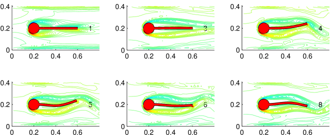
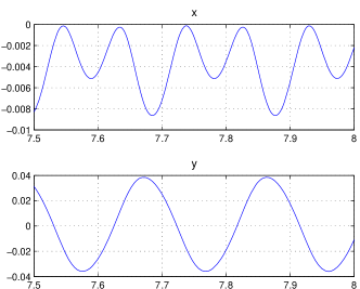
For case (II), we use elements and take to integrate to . The computational mesh is shown in Fig. 4. Some snap-shots of the results are shown in Fig. 5. The time step for case (II) is taken to be small merely for accuracy purpose as our scheme is first order accurate in time. We can take much larger time step. Indeed, we have taken and integrate to for case (II) using the same mesh. The only problem with is accuracy: For example, by the bar with just starts to vibrate while the bar with has already reached its periodic vibrating stage. For case (II), we record the lift and drag forces as well as the position of . In our non-dimensionalized equations, the lift and drag forces are the and components of where is the surface of the cylinder+bar and the is the outward normal with respect to the cylinder+bar. According to [28], the lift and drag forces are and respectively, and the displacements in the and directions of are and respectively. Here we use interval to indicate the range of a periodic oscillating quantity. We stress that we have used our favorite traction type open boundary condition ( where satisfies ) which is physical and allows the bar to contract or expand freely. Moveover, it nails down the arbitrary constant in the fluid pressure [22]. If one prescribes the outflow profile which is the same as the inflow profile, the volume of the bar will keep the same and the arbitrary constant in the pressure will be determined by this constraint. [28] does not state the open boundary condition it uses. If [28] uses Dirichlet type open boundary condition, we expect our results be slightly different from those of [28].


Acknowledgments
The author’s work is supported by the start-up grant from the National University of Singapore with grant number R-146-000-129-133. The author thanks Dr. Stuart Antman and Dr. Jian-Guo Liu for the teaching of continuum mechanics. The author thanks Dr. Long Chen for the finite element package iFEM based on which the finite element calculations in this paper are done. The author thanks Dr. Richard Kollar for helpful discussions.
References
- [1] S. S. Antman, Nonlinear problems of elasticity, 2nd edition, Springer-Verlag, New Tork (2005).
- [2] S. Badia, A. Quaini, and A. Quarteroni, Splitting methods based on algebraic factorization for fluid-structure interaction, SIAM J. Sci. Comput. 30 (2008) 1778–1805.
- [3] J. T. Beale and J. Strain, Locally corrected semi-Lagrangian methods for Stokes flow with moving elastic interfaces, J. Comput. Phys., 227 (2008) 3896–3920
- [4] S. Bönisch, T. Dunne and R. Rannacher, Numerics of fluid-structure interaction, in Lecture Notes of Oberwolfach Seminar ”Hemodynamical Flows: Aspects of Modeling, Analysis and Simoluation”, Nov. 20-26, Oberwolfach (G.P. Galdi, R. Rannacher et al., eds.), Birkhäuser, Basel, 2007.
- [5] P. Causin, J. F. Gerbeau, and F. Nobile, Added-mass effect in the design of partitioned algorithms for fluid-structure peoblems, Comput. Methods Appl. Mech. Engrg. 194 (2005) 4506–4527.
- [6] L. Chen. iFEM: an integrated finite element methods package in MATLAB, Technical Report, University of California at Irvine. 2008.
- [7] L. Chen and C-S. Zhang. A coarsening algorithm on adaptive grids by newest vertex bisection and its applications, Journal of Computational Mathematics, 28 (2010) 767–789.
- [8] P. G. Ciarlet, The finite element method for elliptic problems, Amsterdam, North-Holland, 1978.
- [9] P. G. Ciarlet, Mathematical elasticity, vol. I: three dimensional elasticity, Amsterdam, North Holland, 1988.
- [10] D. Coutand and S. Shkoller, The interaction between quasilinear elastodynamics and the Navier-Stokes equations, Arch. Rational Mech. Anal., 179 (2006) 303–352.
- [11] B. Desjardins and M.J. Esteban, Existence of weak solutions for the motion of rigid bodies in a viscous fluid, Arch. Rational Mech. Anal., 146 (1999) 59- 71.
- [12] C. Farhat, K. G. van der Zee and P. Geuzaine, Provably second-order time-accurate loosely-coupled solution algorithms for transient nonlinear computational aeroelasticity, Comput. Methods Appl. Mech. Eng. 195 (2006) 1973-2001.
- [13] M.A. Fernández, J.-F. Gerbeau and C. Grandmont, A projection semi-implicit scheme for the coupling of an elastic structure with an incompressible fluid Internat. J. Numer. Methods Engrg., 69 (2007) 794 -821.
- [14] L. Formaggia and F. Nobile, A stability analysis for the arbitrary Lagrangian Eulerian formulation with finite elements, East-West J. Numer. Math. 7 (1999) 105–131.
- [15] L. Gerardo-Giorda, F. Nobile, and C. Vergara, Analysis and optimization of Robin-Robin partitioned procedures in fluid-structure interaction problems, SIAM J. Numer. Anal., 48 (2010), 2091–2116
- [16] C. Grandmont, Existence for a three-dimensional steady state fluid-structure interaction problem, J. Math. Fluid Mech., 4 (2002) 76–94.
- [17] G. Guidoboni, R. Glowinski, N. Cavallini, and S. Canic, Stable loosely-coupled-type algorithm for fluid-structure interaction in blood flow, J. Comp. Phys. 228 (2009) 6916–6937.
- [18] J. Hron and S. Turek, A monolithic FEM/multigrid solver for ALE formulation of fluid structure interaction with application in biomechanics. In H.-J. Bungartz and M. Schäfer, editors, Fluid-Structure Interaction: Modelling, Simulation, Optimisation, LNCSE. Springer, 2006.
- [19] R. J. LeVeque and Z. Li, Immersed interface methods for Stokes flow with elastic boundaries or surface tension, SIAM J. Sci. Comput. 18 (1997) 709- 735.
- [20] M. Lenoir, Optimal isoparametric finite elements and error estimates for domains involvling curved boundaries, SIAM J. Numer. Anal. 23 (1986) 562–580.
- [21] J. Liu, Method of curved lines: simple and efficient schemes with provable temporal accuracy up to 5th order for the Stokes equations on a time varying domain. submitted.
- [22] J. Liu, Open and traction boundary conditions for the incompressible Navier Stokes equations, J. Comp. Phys., 228 (2009) 7250 -7267.
- [23] A. Masud, A space-time finite element method for fluid-structure interaction, Ph.D. Thesis, Stanford University (1993).
- [24] P.-O. Persson, G. Strang, A simple mesh generator in MATLAB. SIAM Review 46 (2004) 329–345.
- [25] C. Peskin, The immersed boundary method, Acta Numer. 11 (2002) 479 -517.
- [26] R. Scott, Finite element techniques for curved boundaries, Ph.D. Thesis, Massachusetts Institute of Technology, Cambridge, (1973)
- [27] R. Temam, Navier-Stokes equations. Theory and numerical analysis. Reprint of the 1984 edition. AMS Chelsea Publishing, Providence, R.I., 2001
- [28] S. Turek and J. Hron. Proposal for numerical benchmarking of fluidstructure interaction between an elastic object and laminar incompressible flow. In H.-J. Bungartz and M. Schäfer, editors, Fluid-Structure Interaction: Modelling, Simulation, Optimisation, LNCSE. Springer, 2006.
- [29] S. O. Unverdi and G. Tryggvason, A front-tracking method for viscous, incompressible, multi-fluid flows, J. Comp. Phys., 100 (1992), 25–37.