High Order Maximum Principle Preserving Semi-Lagrangian Finite Difference WENO schemes for the Vlasov Equation

Tao Xiong Jing-Mei Qiu Zhengfu Xu Andrew Christlieb

Abstract

In this paper, we propose the parametrized maximum principle preserving (MPP) flux limiter, originally developed in [Z. Xu, Math. Comp., (2013), in press], to the semi-Lagrangian finite difference weighted essentially non-oscillatory scheme for solving the Vlasov equation. The MPP flux limiter is proved to maintain up to fourth order accuracy for the semi-Lagrangian finite difference scheme without any time step restriction. Numerical studies on the Vlasov-Poisson system demonstrate the performance of the proposed method and its ability in preserving the positivity of the probability distribution function while maintaining the high order accuracy.

Keywords: Semi-Lagrangian method; Finite difference WENO scheme; Maximum principle preserving; Parametrized flux limiter; Vlasov equation

1 Introduction

In this paper, we will consider the Vlasov-Poisson (VP) system

$$\partial_{t}f+{\bf v}\cdot\nabla_{\bf x}f+E(t,{\bf x})\cdot\nabla_{\bf v}f=0,$$ (1.1)

$$E(t,{\bf x})=-\nabla\phi(t,{\bf x}),\qquad-\Delta\phi(t,{\bf x})=\rho(t,{\bf x}).$$ (1.2)

on the domain $(0,T]\times\Omega$, where $\Omega=\Omega_{\bf x}\times\mathbb{R}^{n}$ and $\Omega_{\bf x}\subset\mathbb{R}^{n}$. It is an important system for modelling the collisionless plasma. The Vlasov equation (1.1) is a kinetic equation that describes the time evolution of the probability distribution function (PDF) $f(t,{\bf x},{\bf v})$ of finding an electron at position ${\bf x}$ with velocity ${\bf v}$ at time $t$. $E(t,{\bf x})$ is the electric field and $\phi(t,{\bf x})$ is a self-consistent electrostatic potential function described by the Poisson equation (1.2). The probability distribution function $f$ is coupled with the long range fields via the charge density $\rho(t,{\bf x})=\int_{\mathbb{R}^{n}}f(t,{\bf x},{\bf v})d{\bf v}-1$, with uniformly distributed infinitely massive ions in the background. The total charge neutrality condition $\int_{\Omega_{\bf x}}(\rho(t,{\bf x})-1)d{\bf x}=0$ is imposed. The Vlasov equation (1.1) in the hyperbolic form enjoys the maximum principle preserving (MPP) and positivity preserving (PP) properties. That is, let

$$f_{m}=\underset{x,v}{\text{min}}(f(x,v,0))\geq 0,\quad f_{M}=\underset{x,v}{\text{max}}(f(x,v,0)),$$

the solution at later time is still within the interval $[f_{m},f_{M}]$ and stays positive.

The VP system has been extensively studied numerically. Popular numerical methods, besides the semi-Lagrangian (SL) approaches which will be reviewed in the next paragraph, include particle-in-cell (PIC) methods [12, 5, 20], Lagrangian particle methods [4, 13], weighted essentially non-oscillatory (WENO) coupled with Fourier collocation [42], Fourier-Fourier spectral methods [23, 22], finite volume methods [14, 16], continuous finite element methods [39, 38], Runge-Kutta discontinuous Galerkin methods [19, 3, 11, 9, 8], and methods in references therein.

In this paper, we focus on the SL method, which has been proposed and applied for a wide range of applications, e.g. in atmospheric modeling and simulations [32, 17], in capturing the moving interface via solving level set equations [33], in fluid dynamics [36] and in kinetic simulations [15, 34]. Compared to the Eulerian approach, the SL approach also has a fixed set of numerical meshes, but in each time step evolution, the information propagates along the characteristics in the Lagrangian fashion. The SL method can be designed as accurate as the Eulerian approach. In addition, the SL method is free of time step restriction by utilizing the characteristic method in the temporal direction. The design of SL approach requires the tracking of characteristics forward or backward in time, which could be challenging for nonlinear problems. To avoid such difficulty in solving the VP system, the dimensional splitting approach was proposed in [7]. Along this line, SL methods were developed in various settings. For example, in the finite difference framework, different interpolation strategies, such as the cubic spline interpolation [31], the cubic interpolated propagation [25], the high order WENO interpolation in a non-conservative form [6] and in a conservative form [26, 27, 28] are proposed. There have also been many work in designing the SL methods in the finite volume framework for the VP system [16] and for the guiding center Vlasov model [10], in the finite element discontinuous Galerkin (DG) framework [30, 29] and with a hybrid finite difference-finite element approach [18].

Our main interest in this paper is to develop a MPP, and in particular PP, SL finite difference WENO scheme for the VP system (1.1). The main challenge of designing MPP (and/or PP) schemes within the SL WENO framework is to maintain the designed high order of accuracy from the conservative WENO approximation. Meanwhile, it is desired that no additional restrictive CFL constraint will be introduced. There have been some research efforts on designing MPP and PP high order SL schemes. For example, in [16, 10], PP property is preserved in the finite volume framework. However, the PP preservation of the PDF is accompanied with sacrificing high order spatial accuracy. Recently, in [30, 29], the SL discontinuous Galerkin (DG) methods to solve the VP system is coupled with the MPP limiters, that were originally proposed by Zhang and Shu [40]. In these approaches, the limiters are applied to the reconstructed polynomials (for finite volume) or the representing polynomials (for DG). In general, the MPP (or PP) property together with the maintenance of high order accuracy is much more challenging to achieve in the finite difference framework than in the finite volume and finite element DG framework via limiting polynomials, see [41].

We propose to generalize the recently developed parametrized MPP flux limiter [37] to a conservative SL finite difference WENO method solving the VP system. The original parametrized flux limiter for 1D scalar conservation laws was later extended to the two-dimensional case [24]. Xiong et al. [35] proposed to apply the parametrized MPP flux limiter to the final Runge-Kutta (RK) stage only, with significantly improved time step restriction for maintenance of high order accuracy, leading to much reduced computational cost. It has also been proved in [35] that the parametrized MPP flux limiter can maintain up to third order accuracy both in space and in time for nonlinear scalar conservation laws.

In order to apply the parametrized MPP flux limiter in [37] for solving the VP system, we start with the dimensional splitting approach. The parametrized MPP flux limiter is proposed for the conservative high order SL finite difference WENO scheme [27, 26]. We mimic the proof in [35] to prove that the parametrized MPP flux limiter for the SL finite difference scheme solving linear advection equations can maintain up to fourth order accuracy without any time step constraint. We also apply the parametrized flux limiter proposed in [35] to the RK finite difference WENO approximation of the VP system without operator splitting. Through numerical studies on weak and strong Landau damping, two stream instabilities, and KEEN waves, we show that both methods perform very well with the designed MPP properties, while maintaining high order accuracy and mass conservation.

The rest of the paper is organized as follows. In Section 2, the SL finite difference WENO scheme is reviewed and the parametrized MPP flux limiting procedure is proposed for the SL WENO scheme. We also prove that the parametrized MPP flux limiter maintains up to fourth order accuracy without additional time step restriction. Numerical studies of the scheme are presented in Section 3. Conclusions are made in Section 4.

2 The parametrized MPP flux limiter for the SL WENO scheme

In this section, we will briefly describe the SL finite difference WENO scheme for solving Vlasov equation (1.1) in one dimension (both physical and phase spaces). We adopt the method in [28], which is in a conservative flux difference form and is suitable to be coupled with the newly developed parametrized MPP flux limiter [37].

For the one-dimensional problem, periodic boundary conditions are imposed in x-direction on a finite domain $\Omega_{x}=[0,L]$ and in v-direction with a cut-off domain $[-V_{c},V_{c}]$ with $V_{c}$ chosen to be large enough to guarantee $f(x,v,t)=0$ for $|v|\geq V_{c}$. The domain $\Omega=[0,L]\times[-V_{c},V_{c}]$ is discretized by the the computational grid

$$0=x_{\frac{1}{2}}<x_{\frac{3}{2}}<\cdots<x_{N_{x}+\frac{1}{2}}=L,\quad-V_{c}=v_{\frac{1}{2}}<v_{\frac{3}{2}}<\cdots<v_{N_{v}+\frac{1}{2}}=V_{c}.$$

Let $x_{i}=\frac{1}{2}(x_{i-\frac{1}{2}}+x_{i+\frac{1}{2}})$ and $v_{j}=\frac{1}{2}(v_{j-\frac{1}{2}}+v_{j+\frac{1}{2}})$ to be the middle point of each cell. The uniform mesh sizes in each direction are $\Delta x=x_{i+\frac{1}{2}}-x_{i-\frac{1}{2}}$ and $\Delta v=v_{j+\frac{1}{2}}-v_{j-\frac{1}{2}}$.

Following [7], the Vlasov equation is dimensionally split to the following form

$$\partial_{t}f+v\cdot\nabla_{x}f=0,$$ (2.1)

$$\partial_{t}f+E(t,x)\cdot\nabla_{v}f=0.$$ (2.2)

Using the second order Strang splitting strategy, the numerical solution is updated from time level $t^{n}$ to time level $t^{n+1}$ by solving equation (2.1) for half a time step, then solving equation (2.2) by a full time step, followed by solving equation (2.1) for another half a time step. Note that each split equation (2.1) or (2.2) still preserves the MPP (and/or PP) property.

In the following, we will take the prototype 1D linear advection equation

$$u_{t}+au_{x}=0$$ (2.3)

with constant $a$, to present the SL finite difference scheme with the parametrized MPP flux limiters.

2.1 Review of SL finite difference WENO scheme

The SL finite difference WENO scheme proposed in [28] is based on integrating equation (2.3) in time over $[t^{n},t^{n+1}]$,

$$u(x,t^{n+1})=u(x,t^{n})-\mathcal{F}(x)_{x},$$ (2.4)

where

$$\mathcal{F}(x)=\int_{t^{n}}^{t^{n+1}}au(x,\tau)d\tau.$$ (2.5)

By introducing a sliding average function $\mathcal{H}(x)$

$$\mathcal{F}(x)=\frac{1}{\Delta x}\int_{x-\frac{\Delta x}{2}}^{x+\frac{\Delta x}{2}}\mathcal{H}(\zeta)d\zeta,$$ (2.6)

with

$$\mathcal{F}(x)_{x}=\frac{1}{\Delta x}\left(\mathcal{H}(x+\frac{\Delta x}{2})-\mathcal{H}(x-\frac{\Delta x}{2})\right),$$ (2.7)

the evaluation of equation (2.4) at the grid point $x_{i}$ can be written in a conservative form

$$u^{n+1}_{i}=u^{n}_{i}-\frac{1}{\Delta x}\left(\mathcal{H}(x_{i+\frac{1}{2}})-\mathcal{H}(x_{i-\frac{1}{2}})\right),$$ (2.8)

where $\mathcal{H}(x_{i+\frac{1}{2}})$ is called the flux function. A SL finite difference WENO reconstruction is used to approximate the numerical flux function $\mathcal{H}(x_{i+\frac{1}{2}})$ based on its cell averages

$$\bar{\mathcal{H}}_{j}=\frac{1}{\Delta x}\int_{x_{j-\frac{1}{2}}}^{x_{j+\frac{1}{2}}}\mathcal{H}(\zeta)d\zeta,\quad j=i-p,\cdots,i+q,$$ (2.9)

with

$$\bar{\mathcal{H}}_{j}=\mathcal{F}(x_{j})=\int_{x^{\star}_{j}}^{x_{j}}u(\zeta,t^{n})d\zeta,$$

where $x^{\star}_{j}=x_{j}-a\Delta t$ is the point tracing from the grid point $(x_{j},t^{n+1})$ along characteristics back to the time level $t^{n}$. The last equality above is essential for the SL scheme, and is obtained via following characteristics. $\int_{x^{\star}_{j}}^{x_{j}}u(\zeta,t^{n})d\zeta$ can be reconstructed from $\{u^{n}_{i}\}^{N_{x}}_{i=1}$ for each $j$. In summary, the SL finite difference WENO scheme procedure in evolving equation (2.3) from $t_{n}$ to $t_{n+1}$ is as follows:

1. At each of the grid points at time level $t^{n+1}$, say $(x_{i},t^{n+1})$, trace the characteristic back to time level $t_{n}$ at $x^{\star}_{i}=x_{i}-a\Delta t$.

2. Reconstruct $\mathcal{F}(x_{i})=\int_{x_{i}^{\star}}^{x_{i}}u(\zeta,t^{n})d\zeta$ from $\{u^{n}_{j}\}_{j=1}^{N_{x}}$. We use $\mathcal{R}_{1}$ to denote this reconstruction procedure

   $$\mathcal{R}_{1}[x_{i}^{\star},x_{i}](u^{n}_{i-p_{1}},\cdots,u^{n}_{i+q_{1}}),$$ (2.10)

   to approximate $\mathcal{F}(x_{i})$, where $(i-p_{1},\cdots,i+q_{1})$ indicates the stencil used in the reconstruction. $\mathcal{R}_{1}[a,b]$ indicates the reconstruction of $\int_{a}^{b}u(\zeta,t)d\zeta$.

3. Reconstruct $\{\mathcal{H}(x_{i+\frac{1}{2}})\}_{i=0}^{N_{x}}$ from $\{\bar{\mathcal{H}}_{i}\}_{i=1}^{N_{x}}$. We use $\mathcal{R}_{2}$ to denote this reconstruction procedure

   $$\mathcal{H}_{i+\frac{1}{2}}\doteq\mathcal{R}_{2}(\bar{\mathcal{H}}_{i-p_{2}},\cdots,\bar{\mathcal{H}}_{i+q_{2}}),$$ (2.11)

   to approximate $\mathcal{H}(x_{i+\frac{1}{2}})$. Here $(i-p_{2},\cdots,i+q_{2})$ indicates the stencil used in the reconstruction.

4. Update the solution $\{u^{n+1}_{i}\}_{i=1}^{N_{x}}$ by

   $$u^{n+1}_{i}=u^{n}_{i}-\frac{1}{\Delta x}(\mathcal{H}_{i+\frac{1}{2}}-\mathcal{H}_{i-\frac{1}{2}}),$$ (2.12)

   with numerical fluxes $\mathcal{H}_{i\pm\frac{1}{2}}$ computed in the previous step.

When the reconstruction stencils in $\mathcal{R}_{1}$ and $\mathcal{R}_{2}$ above only involve one neighboring point value of the solution, then the scheme reduces to a first order monotone scheme when the time step is within CFL restriction. We let $h_{i+\frac{1}{2}}$ denote the first order flux. The proposed SL finite difference scheme can be designed to be of high order accuracy by including more points in the stencil for $\mathcal{R}_{2}\circ\mathcal{R}_{1}$ (the composition of $\mathcal{R}_{1}$ and $\mathcal{R}_{2}$), to reconstruct the numerical flux

$$\mathcal{H}_{i+\frac{1}{2}}=\mathcal{R}_{2}\circ\mathcal{R}_{1}(u^{n}_{i-p},\cdots,u^{n}_{i+q}),$$ (2.13)

where $(i-p,\cdots,i+q)$ indicates the stencil used in the reconstruction process. The WENO mechanism can be introduced in the reconstruction procedures in order to realize a stable and non-oscillatory capture of fine scale structures. In the Appendix, we provide formulas to obtain the high order fluxes $\mathcal{H}_{i+\frac{1}{2}}$ in (2.13) for the fifth order SL finite difference WENO scheme. For more details, we refer to [28].

For the case of large time step $|a|\Delta t>\Delta x$, if $a>0$, $x^{\star}_{i}=x_{i}-a\Delta t$ is no longer inside $(x_{i-1},x_{i}]$, let $i^{\star}$ to be the index such that $x^{\star}_{i}\in(x_{i^{\star}-1},x_{i^{\star}}]$ and $\xi=\frac{x_{i^{\star}}-x^{\star}_{i}}{\Delta x}$, we have

$$h_{i+\frac{1}{2}} = \sum_{j=i^{\star}+1}^{i}\Delta xu^{n}_{j}+(x_{i^{\star}}-x^{\star}_{i})u^{n}_{i^{\star}},$$ (2.14)

$$\mathcal{H}_{i+\frac{1}{2}} = \sum_{j=i^{\star}+1}^{i}\Delta xu^{n}_{j}+\mathcal{H}_{i^{\star}+\frac{1}{2}},$$ (2.15)

where $\mathcal{H}_{i^{\star}+\frac{1}{2}}$ is reconstructed in the same fashion as (2.13), but replacing $i$ by $i^{\star}$. Similarly, if $a<0$, let $i^{\star}$ to be the index such that $x^{\star}_{i}\in(x_{i^{\star}},x_{i^{\star}+1}]$ and $\xi=\frac{x_{i^{\star}}-x^{\star}_{i}}{\Delta x}$, we have

$$h_{i+\frac{1}{2}} = -\sum_{j=i+1}^{i^{\star}}\Delta xu^{n}_{j}+(x_{i^{\star}}-x^{\star}_{i})u^{n}_{i^{\star}+1},$$ (2.16)

$$\mathcal{H}_{i+\frac{1}{2}} = -\sum_{j=i+1}^{i^{\star}}\Delta xu^{n}_{j}+\mathcal{H}_{i^{\star}+\frac{1}{2}}.$$ (2.17)

It is numerically demonstrated in [28] that the proposed high order SL WENO method works very well in Vlasov simulations with extra large time step evolution.

2.2 Parametrized MPP flux limiters

In this subsection, we propose a parametrized MPP flux limiter, as proposed in [37, 35], for the high order SL finite difference WENO scheme (2.12).

For simplicity, Let $u_{m}=\underset{x}{\text{min}}(u(x,0))$ and $u_{M}=\underset{x}{\text{max}}(u(x,0))$ as the minimum and maximum values of the initial condition. It has been known that the numerical solutions updated by (2.12) with the first order monotone flux satisfy the maximum principle. The MPP flux limiters are designed as modifying the high order numerical flux towards the first order monotone flux in the following way,

$$\tilde{\mathcal{H}}_{i+\frac{1}{2}}=\theta_{i+\frac{1}{2}}(\mathcal{H}_{i+\frac{1}{2}}-h_{i+\frac{1}{2}})+h_{i+\frac{1}{2}}$$ (2.18)

where $\theta_{i+\frac{1}{2}}\in[0,1]$ is the parameter to be designed to take advantage of the first order monotone flux $h_{i+\frac{1}{2}}$ in the MPP property and to take advantage of the high order flux $\mathcal{H}_{i+\frac{1}{2}}$ in the high order accuracy.

Below is a detailed procedure of designing $\theta_{i+\frac{1}{2}}$, in order to guarantee the MPP property of the numerical solutions, yet to choose $\theta_{i+\frac{1}{2}}$’s to be as close to $1$ as possible for high order accuracy. For each $\theta_{i+\frac{1}{2}}$ in limiting the numerical flux $\tilde{\mathcal{H}}_{i+\frac{1}{2}}$ as in equation (2.18), we are looking for the upper bounds $\Lambda_{+\frac{1}{2},I_{i}}$ and $\Lambda_{-\frac{1}{2},I_{i+1}}$, such that, for all

$$\theta_{i+\frac{1}{2}}\in[0,\Lambda_{+\frac{1}{2},I_{i}}]\cap[0,\Lambda_{-\frac{1}{2},I_{i+1}}],$$ (2.19)

the updated numerical solutions $u^{n+1}_{i}$ and $u^{n+1}_{i+1}$ by the SL WENO scheme (2.12) with the modified numerical fluxes (2.18) are within $[u_{m},u_{M}]$. Let

$$\Gamma^{M}_{i}=u_{M}-u^{n}_{i}+\frac{1}{\Delta x}(h_{i+\frac{1}{2}}-h_{i-\frac{1}{2}}),\quad\Gamma^{m}_{i}=u_{m}-u^{n}_{i}+\frac{1}{\Delta x}(h_{i+\frac{1}{2}}-h_{i-\frac{1}{2}}),$$

the MPP property of the first order monotone flux guarantees

$$\Gamma^{M}_{i}\geq 0,\quad\Gamma^{m}_{i}\leq 0.$$ (2.20)

To ensure $u^{n+1}_{i}\in[u_{m},u_{M}]$ with $\tilde{\mathcal{H}}_{i+\frac{1}{2}}$ as in equation (2.18), it is sufficient to have

$$\frac{1}{\Delta x}\theta_{i-\frac{1}{2}}(\mathcal{H}_{i-\frac{1}{2}}-h_{i-\frac{1}{2}})-\frac{1}{\Delta x}\theta_{i+\frac{1}{2}}(\mathcal{H}_{i+\frac{1}{2}}-h_{i+\frac{1}{2}})-\Gamma^{M}_{i} \leq 0,$$ (2.21)

$$\frac{1}{\Delta x}\theta_{i-\frac{1}{2}}(\mathcal{H}_{i-\frac{1}{2}}-h_{i-\frac{1}{2}})-\frac{1}{\Delta x}\theta_{i+\frac{1}{2}}(\mathcal{H}_{i+\frac{1}{2}}-h_{i+\frac{1}{2}})-\Gamma^{m}_{i} \geq 0.$$ (2.22)

The linear decoupling of $\theta_{i\pm\frac{1}{2}}$, subject to the constraints (2.21) and (2.22), is achieved via a case-by-case discussion based on the sign of

$$F_{i\pm\frac{1}{2}}\doteq\frac{1}{\Delta x}\left(\mathcal{H}_{i\pm\frac{1}{2}}-h_{i\pm\frac{1}{2}}\right),$$

as outlined below.

1. Assume

   $$\theta_{i-\frac{1}{2}}\in[0,\Lambda^{M}_{-\frac{1}{2},I_{i}}],\quad\theta_{i+\frac{1}{2}}\in[0,\Lambda^{M}_{+\frac{1}{2},I_{i}}],$$

   where $\Lambda^{M}_{-\frac{1}{2},I_{i}}$ and $\Lambda^{M}_{+\frac{1}{2},I_{i}}$ are the upper bounds of $\theta_{i\pm\frac{1}{2}}$, subject to the constraint (2.21).

   1. If $F_{i-\frac{1}{2}}\leq 0$ and $F_{i+\frac{1}{2}}\geq 0$,

      $$(\Lambda^{M}_{-\frac{1}{2},I_{i}},\Lambda^{M}_{+\frac{1}{2},I_{i}})=(1,1).$$

   2. If $F_{i-\frac{1}{2}}\leq 0$ and $F_{i+\frac{1}{2}}<0$,

      $$(\Lambda^{M}_{-\frac{1}{2},{I_{i}}},\Lambda^{M}_{+\frac{1}{2},{I_{i}}})=(1,\min(1,\frac{\Gamma^{M}_{i}}{-F_{i+\frac{1}{2}}})).$$

   3. If $F_{i-\frac{1}{2}}>0$ and $F_{i+\frac{1}{2}}\geq 0$,

      $$(\Lambda^{M}_{-\frac{1}{2},{I_{i}}},\Lambda^{M}_{+\frac{1}{2},{I_{i}}})=(\min(1,\frac{\Gamma^{M}_{i}}{F_{i-\frac{1}{2}}}),1).$$

   4. If $F_{i-\frac{1}{2}}>0$ and $F_{i+\frac{1}{2}}<0$,

      • If equation (2.21) is satisfied with $(\theta_{i-\frac{1}{2}},\theta_{i+\frac{1}{2}})=(1,1)$, then

        $$(\Lambda^{M}_{-\frac{1}{2},{I_{i}}},\Lambda^{M}_{+\frac{1}{2},{I_{i}}})=(1,1).$$

      • Otherwise,

        $$(\Lambda^{M}_{-\frac{1}{2},{I_{i}}},\Lambda^{M}_{+\frac{1}{2},{I_{i}}})=(\frac{\Gamma^{M}_{i}}{F_{i-\frac{1}{2}}-F_{i+\frac{1}{2}}},\frac{\Gamma^{M}_{i}}{F_{i-\frac{1}{2}}-F_{i+\frac{1}{2}}}).$$

2. Similarly assume

   $$\theta_{i-\frac{1}{2}}\in[0,\Lambda^{m}_{-\frac{1}{2},I_{i}}],\quad\theta_{i+\frac{1}{2}}\in[0,\Lambda^{m}_{+\frac{1}{2},I_{i}}],$$

   where $\Lambda^{m}_{-\frac{1}{2},I_{i}}$ and $\Lambda^{m}_{+\frac{1}{2},I_{i}}$ are the upper bounds of $\theta_{i\pm\frac{1}{2}}$, subject to the constraint (2.22).

   1. If $F_{i-\frac{1}{2}}\geq 0$ and $F_{i+\frac{1}{2}}\leq 0$,

      $$(\Lambda^{m}_{-\frac{1}{2},I_{i}},\Lambda^{m}_{+\frac{1}{2},I_{i}})=(1,1).$$

   2. If $F_{i-\frac{1}{2}}\geq 0$ and $F_{i+\frac{1}{2}}>0$,

      $$(\Lambda^{m}_{-\frac{1}{2},{I_{i}}},\Lambda^{m}_{+\frac{1}{2},{I_{i}}})=(1,\min(1,\frac{\Gamma^{m}_{i}}{-F_{i+\frac{1}{2}}})).$$

   3. If $F_{i-\frac{1}{2}}<0$ and $F_{i+\frac{1}{2}}\leq 0$,

      $$(\Lambda^{m}_{-\frac{1}{2},{I_{i}}},\Lambda^{m}_{+\frac{1}{2},{I_{i}}})=(\min(1,\frac{\Gamma^{m}_{i}}{F_{i-\frac{1}{2}}}),1).$$

   4. If $F_{i-\frac{1}{2}}<0$ and $F_{i+\frac{1}{2}}>0$,

      • If equation (2.22) is satisfied with $(\theta_{i-\frac{1}{2}},\theta_{i+\frac{1}{2}})=(1,1)$, then

        $$(\Lambda^{m}_{-\frac{1}{2},{I_{i}}},\Lambda^{m}_{+\frac{1}{2},{I_{i}}})=(1,1).$$

      • Otherwise,

        $$(\Lambda^{m}_{-\frac{1}{2},{I_{i}}},\Lambda^{m}_{+\frac{1}{2},{I_{i}}})=(\frac{\Gamma^{m}_{i}}{F_{i-\frac{1}{2}}-F_{i+\frac{1}{2}}},\frac{\Gamma^{m}_{i}}{F_{i-\frac{1}{2}}-F_{i+\frac{1}{2}}}).$$

Notice that the range of $\theta_{i+\frac{1}{2}}$ (2.19) is determined by the need to ensure both the upper bound (2.21) and the lower bound (2.22) of numerical solutions in both cell $I_{i}$ and $I_{i+1}$. Thus the locally defined limiting parameter is given as

$$\theta_{i+\frac{1}{2}}=\min(\Lambda_{+\frac{1}{2},{I_{i}}},\Lambda_{-\frac{1}{2},{I_{i+1}}}),$$ (2.23)

with $\Lambda_{+\frac{1}{2},{I_{i}}}=\min(\Lambda^{M}_{+\frac{1}{2},{I_{i}}},\Lambda^{m}_{+\frac{1}{2},{I_{i}}})$ and $\Lambda_{-\frac{1}{2},{I_{i+1}}}=\min(\Lambda^{M}_{-\frac{1}{2},{I_{i+1}}},\Lambda^{m}_{-\frac{1}{2},{I_{i+1}}})$. The modified flux in equation (2.18) with the $\theta_{i+\frac{1}{2}}$ designed above ensures the maximum principle. Such modified flux is consistent and preserves the maximum principle by its design, since it is a convex combination ($\theta_{i+\frac{1}{2}}\in[0,1]$) of a high order flux $\mathcal{H}_{i+\frac{1}{2}}$ and the first order flux $h_{i+\frac{1}{2}}$. The mass conservation property is preserved, due to the flux difference form of the scheme.

Remark 2.1.

(Machine zero) Due to rounding floating point arithmetic, equations (2.20), (2.21) and (2.22) are enforced only at the level of machine precision. In some extreme cases, numerical solutions may go out of bound, but only at the level of machine precision.

In [35], it was proved that the MPP flux limiter for the RK finite difference scheme can maintain up to third order accuracy both in space and in time for the nonlinear scalar equation $u_{t}+f(u)_{x}=0$. In Theorem 2.2 below, we prove the proposed MPP limiter for the SL finite difference scheme can maintain up to fourth order accuracy for solving the linear advection equation (2.3) without any time step restriction. The generalization of the proof to maintain up to fifth order accuracy would be much more technical and will be investigated in our future work.

Theorem 2.2.

Consider solving the linear advection equation (2.3) using the finite difference SL method (2.12) with a fourth order reconstruction procedure. Assume the global error,

$$e^{n}_{j}=|u^{n}_{j}-u(x_{j},t^{n})|=\mathcal{O}(\Delta x^{4}),\quad\forall n,j.$$ (2.24)

Consider applying the parametrized MPP flux limiter to the numerical fluxes, then

$$\left|\frac{1}{\Delta x}\left(\mathcal{H}_{j+\frac{1}{2}}-\tilde{\mathcal{H}}_{j+\frac{1}{2}}\right)\right|=\mathcal{O}(\Delta x^{4}),\quad\forall j,$$ (2.25)

without any time step restriction.

Proof.

Without loss of generality, we consider $a=1$ with $0\leq\xi=\frac{\Delta t}{\Delta x}\leq 1$. The case of $\Delta t>\Delta x$ can be reduced to $\Delta t\leq\Delta x$ by shifting the numerical solution with several whole grid points. Without specifying, in the following, we use $u_{j}$ instead of $u^{n}_{j}$ and use $u(x)$ instead of $u(x,t^{n})$. Since the difference between $u(x_{j},t^{n})$ and $u^{n}_{j}$ is of high order due to assumption (2.24), we use $u(x_{j},t^{n})$ and $u^{n}_{j}$ interchangeably when such high order difference allows. The high order flux $\mathcal{H}_{j+\frac{1}{2}}$ is taken to be (2.13) with a 4th order finite difference reconstruction, the first order monotone flux is $h_{j-\frac{1}{2}}=\Delta tu_{j-1}$.

We mimic the proof in [35] and only consider the most challenging case: case (b) for the maximum value part. The proof for other cases would be similar to that in [35].

We consider case (b) when

$$\Lambda_{+\frac{1}{2},{I_{j}}}=\frac{\Gamma^{M}_{j}}{-F_{j+\frac{1}{2}}}<1.$$ (2.26)

To prove (2.25), it suffices to prove

$$u_{M}-\left(u_{j}-\xi(\hat{H}_{j+\frac{1}{2}}-u_{j-1})\right)=\mathcal{O}(\Delta x^{4}),$$ (2.27)

if $u_{M}-\left(u_{j}-\xi(\hat{H}_{j+\frac{1}{2}}-u_{j-1})\right)<0$. For the SL method, we have

$$\hat{H}_{j+\frac{1}{2}}=\frac{1}{\Delta t}\mathcal{H}_{j+\frac{1}{2}}=\frac{1}{\Delta t}\int_{t^{n}}^{t^{n+1}}H(x_{j+\frac{1}{2}},\tau)d\tau,$$ (2.28)

where $H(x,t)$ is defined by

$$u(x,t)=\frac{1}{\Delta x}\int^{x+\frac{\Delta x}{2}}_{x-\frac{\Delta x}{2}}H(\xi,t)d\xi.$$ (2.29)

$H(x,t)$ follows the same characteristics as the linear advection equation, hence

$$\hat{H}_{j+\frac{1}{2}}=\frac{1}{\Delta t}\int_{0}^{\Delta t}H(x_{j+\frac{1}{2}}-\tau,t^{n})d\tau.$$ (2.30)

Let $I_{1}=u_{j}-\xi(\hat{H}_{j+\frac{1}{2}}-u_{j-1})$. We approximate $H(x,t^{n})$ by a 4th order reconstructed polynomial from the solution based on the stencil $S=\{u_{j-2},u_{j-1},u_{j},u_{j+1}\}$, with which

$$I_{1} = u_{j}-\xi\left(\frac{1}{\Delta t}\int_{0}^{\Delta t}H(x_{j+\frac{1}{2}}-\tau,t^{n})d\tau-u_{j-1}\right)$$ (2.31)

$$= \frac{1}{24}(26u_{j}-10u_{j-1}+2u_{j-2}+6u_{j+1})+\frac{\xi}{24}(9u_{j}+3u_{j-1}-u_{j-2}-11u_{j+1})$$

$$+\frac{\xi^{2}}{24}(-14u_{j}+10u_{j-1}-2u_{j-2}+6u_{j+1})+\frac{\xi^{3}}{24}(3u_{j}-3u_{j-1}+u_{j-2}-u_{j+1}).$$

We first consider the case when the maximum point $x_{M}\in(x_{j-1},x_{j})$ at $t^{n}$, with $u_{M}=u(x_{M})$, $u^{\prime}_{M}=0$ and $u^{\prime\prime}_{M}\leq 0$. $(x_{j-1},x_{j})$ is the dependent domain for the exact solution $u(x_{j},t^{n+1})$ when $0\leq\xi\leq 1$. We perform Taylor expansions around $x_{M}$ up to $4$th order and obtain

$$u_{j+1} = u_{M}+u^{\prime}_{M}(x_{j}-x_{M}+\Delta x)+u^{\prime\prime}_{M}\frac{(x_{j}-x_{M}+\Delta x)^{2}}{2}+u^{\prime\prime\prime}_{M}\frac{(x_{j}-x_{M}+\Delta x)^{3}}{6}+\mathcal{O}(\Delta x^{4}),$$

$$u_{j} = u_{M}+u^{\prime}_{M}(x_{j}-x_{M})+u^{\prime\prime}_{M}\frac{(x_{j}-x_{M})^{2}}{2}+u^{\prime\prime\prime}_{M}\frac{(x_{j}-x_{M})^{3}}{6}+\mathcal{O}(\Delta x^{4}),$$

$$u_{j-1} = u_{M}+u^{\prime}_{M}(x_{j}-x_{M}-\Delta x)+u^{\prime\prime}_{M}\frac{(x_{j}-x_{M}-\Delta x)^{2}}{2}+u^{\prime\prime\prime}_{M}\frac{(x_{j}-x_{M}-\Delta x)^{3}}{6}+\mathcal{O}(\Delta x^{4}),$$

$$u_{j-2} = u_{M}+u^{\prime}_{M}(x_{j}-x_{M}-2\Delta x)+u^{\prime\prime}_{M}\frac{(x_{j}-x_{M}-2\Delta x)^{2}}{2}+u^{\prime\prime\prime}_{M}\frac{(x_{j}-x_{M}-2\Delta x)^{3}}{6}+\mathcal{O}(\Delta x^{4}).$$

Since $u^{\prime}_{M}=0$, we can write $I_{1}$ to be

$$I_{1}=u_{M}+u^{\prime\prime}_{M}\frac{\Delta x^{2}}{2}R_{2}+u^{\prime\prime\prime}_{M}\frac{\Delta x^{3}}{6}R_{3}+\mathcal{O}(\Delta x^{4}),$$ (2.32)

where

$$R_{2} = \frac{5}{6}\xi+\frac{1}{2}\xi^{2}-\frac{1}{3}\xi^{3}+(\xi^{2}-3\xi)z+z^{2},$$

$$R_{3} = \frac{1}{4}(-4\xi+\xi^{2}-2\xi^{3}+\xi^{4})+\frac{1}{4}(10\xi+6\xi^{2}-4\xi^{3})z+\frac{1}{4}(-18\xi+6\xi^{2})z^{2}+z^{3},$$

and $z=(x_{j}-x_{M})/\Delta x\in(0,1)$.

We consider a quantity denoted by $I_{2}$, which can be written as follows

$$I_{2} = \beta_{1}u(x_{M})+(1-\beta_{1})u(x_{M}+c_{1}\Delta x)$$ (2.33)

$$= u_{M}+u^{\prime\prime}_{M}\frac{\Delta x^{2}}{2}(1-\beta_{1})c_{1}^{2}+u^{\prime\prime\prime}_{M}\frac{\Delta x^{3}}{6}(1-\beta_{1})c_{1}^{3}+\mathcal{O}(\Delta x^{4}),$$

with parameters $\beta_{1}$ and $c_{1}$ to be determined. If $0\leq\beta_{1}\leq 1$, $I_{2}\leq u_{M}$.

Since $u^{\prime\prime}_{M}\leq 0$, if we can find $c_{1}=\mathcal{O}(1)$, $0\leq\beta_{1}\leq 1$ such that

$$(1-\beta_{1})c_{1}^{2}\leq R_{2},\qquad(1-\beta_{1})c_{1}^{3}=R_{3},$$ (2.34)

we would have

$$|I_{1}-u_{M}|=\mathcal{O}(\Delta x^{4}),$$ (2.35)

when (2.32) is compared with (2.33) under the assumption (2.26), thus proving (2.27) in this case. In the following, to determine the parameters $\beta_{1}$ and $c_{1}$ satisfying (2.34), we first need $(1-\beta_{1})R_{3}^{2}\leq R_{2}^{3}$, that is

$$1-\beta_{1}\leq\min_{0\leq z\leq 1}\left(\frac{R_{2}^{3}}{R_{3}^{2}}\right),\quad\text{with}\quad 0\leq\xi\leq 1.$$ (2.36)

Using Mathematica, we have

$$\min_{0\leq z\leq 1}\left(\frac{R_{2}^{3}}{R_{3}^{2}}\right)=\begin{cases}\frac{54-108\xi+72\xi^{2}-16\xi^{3}}{54-81\xi+27\xi^{2}},&\quad 0\leq\xi\leq\min(|z|^{3},\frac{1}{2}),\\ \frac{1}{2}-\frac{3}{2}\sqrt{\frac{3}{2}}\sqrt{\frac{2-7\xi+9\xi^{2}-5\xi^{3}+\xi^{4}}{27-32\xi+9\xi^{2}}},&\quad\min(|z|^{3},\frac{1}{2})\leq\xi\leq 1,\end{cases}$$ (2.37)

and

$$\frac{64}{81}\leq\frac{54-108\xi+72\xi^{2}-16\xi^{3}}{54-81\xi+27\xi^{2}}\leq 1, \quad\text{if}\quad 0\leq\xi\leq\frac{1}{2},$$ (2.38)

$$0\leq\frac{1}{2}-\frac{3}{2}\sqrt{\frac{3}{2}}\sqrt{\frac{2-7\xi+9\xi^{2}-5\xi^{3}+\xi^{4}}{27-32\xi+9\xi^{2}}}\leq 1, \quad\text{if}\quad 0\leq\xi\leq 1.$$ (2.39)

Thus, we can choose $\beta_{1}=1-\min_{0\leq z\leq 1}\left(\frac{R_{2}^{3}}{R_{3}^{2}}\right)\in[0,1]$. Let $c_{1}=\left(\frac{R_{3}}{1-\beta_{1}}\right)^{1/3}$. Below, we verify that $|c_{1}|$ is bounded.

If $0\leq\xi\leq\min(|z|^{3},\frac{1}{2})$, from (2.38), we have

$$|c_{1}| \leq \left(\frac{\max_{0\leq\xi\leq 1,0\leq z\leq 1}|R_{3}|}{\min_{0\leq\xi\leq\frac{1}{2}}(1-\beta_{1})}\right)^{1/3}\leq\left(\frac{81}{64}\max_{0\leq\xi\leq,0\leq z\leq 1}|R_{3}|\right)^{1/3}\leq 3.$$

Otherwise if $\min(|z|^{3},\frac{1}{2})\leq\xi\leq 1$, we have

$$\frac{R_{3}}{1-\beta_{1}}=\Lambda(\xi)(\frac{1}{4}(-4+\xi-2\xi^{2}+\xi^{3})+\frac{1}{4}(10+6\xi-4\xi^{2})z+\frac{1}{4}(-18+6\xi)z^{2}+\frac{z^{3}}{\xi}),$$ (2.40)

with

$$\frac{216}{125}\leq\Lambda(\xi)=\frac{\xi}{\frac{1}{2}-\frac{3}{2}\sqrt{\frac{3}{2}}\sqrt{\frac{2-7\xi+9\xi^{2}-5\xi^{3}+\xi^{4}}{27-32\xi+9\xi^{2}}}}\leq 2,$$ (2.41)

$$\frac{1}{4}\leq|\frac{1}{4}(-4+\xi-2\xi^{2}+\xi^{3})+\frac{1}{4}(10+6\xi-4\xi^{2})z+\frac{1}{4}(-18+6\xi)z^{2}|\leq 8,$$ (2.42)

$$\left|\frac{z^{3}}{\xi}\right|\leq 2.$$ (2.43)

In this case we also have $|c_{1}|\leq(2(8+2))^{1/3}\leq 3$.

Now if $x_{M}\notin I_{j}$, however there is a local maximum point $x^{loc}_{M}$ inside $(x_{j-1},x_{j})$, the above analysis still holds. Therefore we consider that $u(x)$ reaches its local maximum $u^{loc}_{M}$ at $x^{loc}_{M}=x_{j-1}$ with $u^{\prime}_{j-1}\leq 0$ and $z=(x_{j}-x^{loc}_{M})/\Delta x=(x_{j}-x_{j-1})/\Delta x=1$. Based on the Taylor expansion, we can rewrite (2.31) to be

$$I_{1}=\frac{1}{2}(2-\xi)(1-\xi)I_{3}+\left(1-\frac{1}{2}(2-\xi)(1-\xi)\right)u_{j-1}+\mathcal{O}(\Delta x^{4}),$$ (2.44)

with

$$I_{3}=u_{j-1}+u^{\prime}_{j-1}\Delta x+u^{\prime\prime}_{j-1}\frac{\Delta x^{2}}{2}\frac{3-2\xi}{3}+u^{\prime\prime\prime}_{j-1}\frac{\Delta x^{3}}{6}\frac{1}{2}(2-\xi)(1-\xi).$$ (2.45)

Similar to (2.33), we consider $I_{4}$ with the following form

$$I_{4} = \beta_{2}u(x_{j-1}-\Delta x)+(1-\beta_{2}-\beta_{3})u(x_{j-1})+\beta_{3}u(x_{j-1}+\Delta x)$$

$$= u_{j-1}+(\beta_{3}-\beta_{2})u^{\prime}_{j-1}\Delta x+(\beta_{2}+\beta_{3})u^{\prime\prime}_{j-1}\frac{\Delta x^{2}}{2}+(\beta_{3}-\beta_{2})u^{\prime\prime\prime}_{j-1}\frac{\Delta x^{3}}{6}+\mathcal{O}(\Delta x^{4}),$$

with $\beta_{2},\beta_{3},\beta_{2}+\beta_{3}\in[0,1]$ to be determined. Since $u^{\prime}_{j-1}\leq 0$, comparing (2.45) with (LABEL:aeq421), we would like to find $\beta_{2}$, $\beta_{3}$ satisfying

$$(\beta_{3}-\beta_{2})\leq 1,\quad\beta_{2}+\beta_{3}=\frac{3-2\xi}{3},\quad\beta_{3}-\beta_{2}=\frac{1}{2}(2-\xi)(1-\xi),$$ (2.47)

from which we would have $|I_{3}-u_{M}|=\mathcal{O}(\Delta x^{4})$ under the assumption that $I_{1}\geq u_{M}$ in (2.44), and $I_{4}\leq u_{M}$. It can then be established that $|I_{1}-u_{M}|=\mathcal{O}(\Delta x^{4})$ if $I_{1}\geq u_{M}$. (2.47) can be easily achieved with

$$\beta_{2} = \frac{1}{2}\left(\frac{3-2\xi}{3}+\frac{1}{2}(2-\xi)(1-\xi)\right)=\frac{1}{12}(3-\xi)(4-3\xi),$$ (2.48)

$$\quad\beta_{3} = \frac{1}{2}\left(\frac{3-2\xi}{3}-\frac{1}{2}(2-\xi)(1-\xi)\right)=\frac{1}{12}\xi(5-3\xi).$$ (2.49)

Finally, if $x^{loc}_{M}=x_{j}$ with $u^{\prime}_{j}\geq 0$ and $z=(x_{j}-x^{loc}_{M})/\Delta x=(x_{j}-x_{j})/\Delta x=0$, we have

$$I_{1}=u_{j}+u^{\prime}_{j}\Delta xR_{1}+u^{\prime\prime}_{j}\frac{\Delta x^{2}}{2}R_{2}+u^{\prime\prime\prime}_{j}\frac{\Delta x^{3}}{6}R_{3}+\mathcal{O}(\Delta x^{4}),$$ (2.50)

where

$$R_{1}=-\frac{1}{2}\xi(3-\xi),\quad R_{2}=\frac{1}{6}\xi(5-2\xi)(1+\xi),\quad R_{3}=-\frac{1}{4}\xi(4-\xi+2\xi^{2}-\xi^{3}).$$

Now let

$$I_{5} = \beta_{4}u_{j}+(1-\beta_{4})u(x_{j}+c_{2}\Delta x)$$

$$= u_{j}+(1-\beta_{4})c_{2}u^{\prime}_{j}\Delta x+(1-\beta_{3})c_{2}^{2}u^{\prime\prime}_{j}\frac{\Delta x^{2}}{2}+(1-\beta_{4})c_{2}^{3}u^{\prime\prime\prime}_{j}\frac{\Delta x^{3}}{6}+\mathcal{O}(\Delta x^{4}).$$

Similar to the other cases, since $u^{\prime}_{j}\geq 0$, if we can find $\beta_{4}\in[0,1]$ and $c_{2}$ bounded, such that,

$$(1-\beta_{4})c_{2}\geq R_{1},\quad(1-\beta_{4})c_{2}^{2}=R_{2},\quad(1-\beta_{4})c_{2}^{3}=R_{3},$$ (2.52)

we would have $|I_{1}-u_{M}|=\mathcal{O}(\Delta x^{4})$, if $I_{1}\geq u_{M}$. (2.52) can be satisfied by letting

$$c_{2}=R_{3}/R_{2},\quad\beta_{4}=1-R_{2}/c_{2}^{2},$$ (2.53)

with $|c_{2}|\leq 6/5$ and $\beta_{4}\in[0,1]$. To this end, we have proved (2.27). ∎

3 Numerical simulations

In this section, we test the 5th order SL finite difference WENO scheme with the parametrized MPP flux limiters, denoted as “SL-WL”, to solve the Vlasov equation. We will compare it with the 5th order finite difference WENO scheme with the 4th order RK time discretization and MPP flux limiters in [35], denoted as “RK-WL”. These two methods without MPP flux limiters are denoted to be “SL-WO” and “RK-WO”, respectively. A fast Fourier transform (FFT) method is used to solve the 1D Poisson equation. For the Vlasov equation, the time step at time level $t^{n}$ is chosen to be $\Delta t=CFL/(\alpha_{x}/\Delta x+\alpha^{n}_{v}/\Delta v)$, where $\alpha_{x}=\max_{j}|v_{j}|$ and $\alpha^{n}_{v}=\max_{i}|E(x_{i},t^{n})|$, and we take the CFL number to be $0.8$ for the SL method and $0.6$ for the RK time method, unless specified.

Example 3.1.

In the first example, we take the advection equation

$$\partial_{t}f+\nabla_{x}f+\nabla_{v}f=0,$$ (3.1)

with initial condition

$$f(0,x,v)=\sin^{4}(x+v),$$ (3.2)

and periodic boundary condition on both directions on the domain $[0,2\pi]\times[-\pi,\pi]$, to test the orders of accuracy for the SL WENO scheme with the parametrized MPP flux limiters. In Table 3.1, the $L^{1}$ and $L^{\infty}$ errors and orders are shown for the SL WENO scheme at time $T=1$, here the time step is $\Delta t=CFL\Delta x/2$ with $CFL=0.8$ and $CFL=2.2$. The expected $5th$ order accuracy is observed. With limiters, the numerical solutions are strictly positive with $f_{min}\geq 0$.

Table 3.1: $L^{1}$ and $L^{\infty}$ errors and orders for the advection equation (3.1) with initial condition (3.2) at $T=1$. “WL” denotes the scheme with limiters, “WO” denotes the scheme without limiters. “$f_{min}$” is the minimum numerical solution of the SL WENO schemes. Mesh size $N_{x}=N_{v}=N$.

		$N$	$L^{1}$ error	order	$L^{\infty}$ error	order	$f_{min}$
$CFL=0.8$	WL	40	2.74E-03	–	5.53E-03	–	1.97E-13
		80	2.35E-04	3.55	7.95E-04	2.80	3.48E-05
		160	7.16E-06	5.04	3.51E-05	4.50	1.09E-13
		320	1.95E-07	5.20	8.99E-07	5.29	8.60E-09
	WO	40	2.86E-03	–	6.06E-03	–	-1.76E-03
		80	2.68E-04	3.42	9.67E-04	2.65	-2.20E-04
		160	7.52E-06	5.15	3.42E-05	4.82	-1.03E-05
		320	1.95E-07	5.27	8.99E-07	5.25	-3.75E-08
$CFL=2.2$	WL	40	1.68E-03	–	3.75E-03	–	1.94E-13
		80	9.87E-05	4.09	3.76E-04	3.32	1.25E-05
		160	2.90E-06	5.09	1.51E-05	4.64	3.64E-07
		320	7.61E-08	5.25	3.55E-07	5.41	5.27E-10
	WO	40	1.80E-03	–	3.83E-03	–	-8.45E-04
		80	1.20E-04	3.91	4.91E-04	2.96	-1.21E-04
		160	2.94E-06	5.35	1.50E-05	5.03	-3.21E-06
		320	7.61E-08	5.27	3.55E-07	5.40	-1.48E-08

Example 3.2.

In the second example, we consider the rigid body rotating problem

$$\partial_{t}f-v\nabla_{x}f+x\nabla_{v}f=0.$$ (3.3)

First we choose a similar smooth initial condition as in [18]

$$f(0,x,v)=\begin{cases}\cos^{6}(r),\quad&r<\pi/2,\\ 0,\quad&\text{otherwise}.\end{cases}$$ (3.4)

on the computational domain $[-\pi,\pi]\times[-\pi,\pi]$ with periodic boundary condition on both directions, where $r=\sqrt{x^{2}+y^{2}}$. Similarly as the first example, we use the SL WENO scheme with or without the parametrized MPP flux limiters to compute up to time $T=2\pi$ for a period. In Table 3.2, the $L^{1}$ and $L^{\infty}$ errors and orders are shown for the time step $\Delta t=CFL\Delta x/(2\pi)$ with $CFL=0.8$ and $CFL=2.2$. Due to the symmetric property of the initial condition, the 5th order spatial error dominates. With the limiters, the numerical solutions are strictly positive.

Table 3.2: $L^{1}$ and $L^{\infty}$ errors and orders for the rigid body rotating problem (3.3) with initial condition (3.4) at $T=2\pi$. “WL” denotes the scheme with limiters, “WO” denotes the scheme without limiters. “$f_{min}$” is the minimum numerical solution of the SL WENO schemes. Mesh size $N_{x}=N_{v}=N$.

		$N$	$L^{1}$ error	order	$L^{\infty}$ error	order	$f_{min}$
$CFL=0.8$	WL	40	5.56E-04	–	1.56E-02	–	1.22E-13
		80	3.69E-05	3.91	7.17E-04	4.44	4.44E-14
		160	1.32E-06	4.80	2.31E-05	4.95	4.75E-16
		320	3.82E-08	5.11	7.22E-07	5.00	1.53E-19
	WO	40	5.68E-04	–	1.56E-02	–	-8.32E-05
		80	4.05E-05	3.81	7.17E-04	4.44	-4.48E-05
		160	1.33E-06	4.93	2.31E-05	4.95	-7.41E-08
		320	3.83E-08	5.11	7.22E-07	5.00	-2.63E-09
$CFL=2.2$	WL	40	5.31E-04	–	1.55E-02	–	1.83E-13
		80	3.62E-05	3.88	7.07E-04	4.46	8.45E-15
		160	1.29E-06	4.81	2.28E-05	4.96	7.54E-18
		320	3.72E-08	5.11	7.10E-07	5.00	1.89E-23
	WO	40	5.44E-04	–	1.55E-02	–	-8.45E-05
		80	3.97E-05	3.78	7.07E-04	4.46	-4.45E-05
		160	1.29E-06	4.94	2.28E-05	4.96	-7.03E-08
		320	3.73E-08	5.11	7.10E-07	5.00	-2.49E-09

Then we consider the initial condition that includes a slotted disk, a cone as well as a smooth hump on the computational domain $[-\pi,\pi]\times[-\pi,\pi]$ as in [35], see Fig. 3.1. For this example, in order to clearly observe the difference of the scheme between with and without the MPP flux limiters, we use the SL WENO scheme but with the linear weights (A.6) and (A.12) instead of the nonlinear weights (A.7). In Fig. 3.2, we display the cuts of the numerical solution at $T=12\pi$ under the time step $\Delta t=CFL\Delta x/(2\pi)$ with $CFL=0.8$. With limiters, the numerical solutions are within the range of $[0,1]$; they are not if without limiters, similar to the results of the RK WENO method with linear weights in [35]. For the results of the SL WENO scheme with nonlinear weights, the minimum and maximum values of the numerical solutions are $0.0000000000000$ and $0.9999999999998$ up to $13$ decimal places, while they are $-0.0020444053893$ and $1.014419874020$ if without limiters. We omit the figures to save space.

,

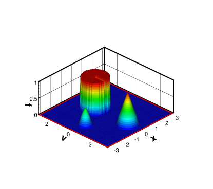
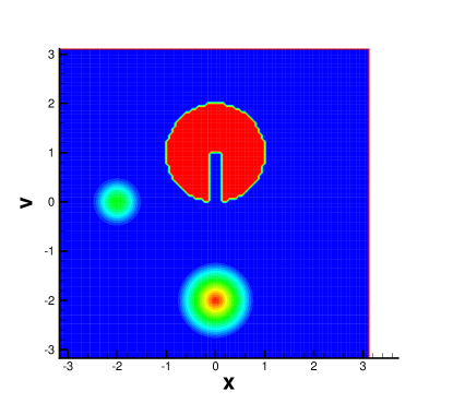
Figure 3.1: The initial profile for equation (3.3). $N_{x}\times N_{v}=100\times 100$.

,
,
,

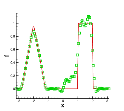
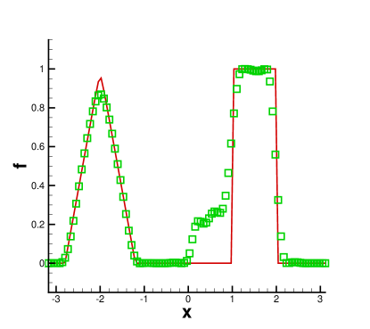
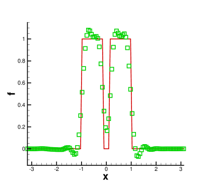
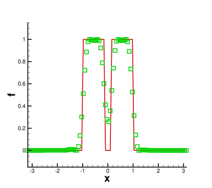
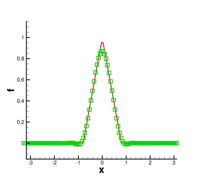
Figure 3.2: Slides of numerical solutions for equation (3.3) with initial condition in Fig. 3.1 at $T=12\pi$. $N_{x}\times N_{v}=100\times 100$. Left: without limiter; Right: with limiter. Cuts along $x=0$, $y=0.8$ and $y=-2$ from top to bottom, respectively. Solid line: exact solution; Symbols: numerical solution.

Next, we consider solving the VP system (1.1) and (1.2). Some classical quantities for the probability distribution function are known to be conserved in time:

• $L^{p}$ norm, $1\leq p\leq\infty$:

  $$\|f\|_{p}=\left(\int_{x}\int_{v}|f(t,x,v)|^{p}dxdv\right)^{1/p},$$ (3.5)

• Energy:

  $$\text{Energy}=\int_{v}\int_{x}f(t,x,v)v^{2}dxdv+\int_{x}E^{2}(t,x)dx,$$ (3.6)

• Entropy:

  $$\text{Entropy}=\int_{v}\int_{x}f(t,x,v)log(f(x,v,t))dxdv.$$ (3.7)

In our simulations, we measure the evolution of these quantities to demonstrate its good performance. With the parametrized MPP flux limiter, the numerical solution of $f(t,x,v)$ would be nonnegative, and the numerical schemes are also conservative themselves, the $L^{1}$ norm is expected to be a constant up to the machine error. Schemes without the MPP flux limiters may produce negative $f(t,x,v)$ somewhere, and could not conserve the $L^{1}$ norm. In the following computation, we take $V_{C}=2\pi$ unless otherwise specified, and the mesh is $N_{x}=80$ and $N_{v}=160$ with periodic boundary conditions on both directions.

Example 3.3.

We first consider the VP system, with the following initial condition:

$$f(0,x,v)=\frac{1}{\sqrt{2\pi}}\cos^{4}(kx)\exp(-\frac{v^{2}}{2}),$$ (3.8)

with periodic boundary condition on both directions on the computational domain $[0,L]\times[-V_{c},V_{c}]$, where $k=0.5$ and $L=2\pi/k=4\pi$. This example is specifically designed to demonstrate that high order accuracy of the original SL scheme is preserved with the MPP flux limiter when solving the VP system. We take $V_{c}=20$ to minimize the error from the domain cutoff. In Table 3.3, the $L^{1}$ and $L^{\infty}$ errors and orders are shown for the SL WENO scheme with $CFL=0.8$ and $CFL=2.2$ at $T=0.01$. $5th$ order accuracy is observed for both $CFL$ conditions. The minimum numerical solutions $f_{min}$ are around machine error if with limiters, otherwise it could be negative.

Table 3.3: $L^{1}$ and $L^{\infty}$ errors and orders for the VP system (1.1) and (1.2) with initial condition (3.8) at $T=0.01$. “WL” denotes the scheme with limiters, “WO” denotes the scheme without limiters. “$f_{min}$” is the minimum of the numerical solution of the SL WENO schemes. Mesh size $N_{v}=2N_{x}$.

		$N_{x}$	$L^{1}$ error	order	$L^{\infty}$ error	order	$f_{min}$
$CFL=0.8$	WL	40	1.07E-06	–	5.22E-05	–	4.60E-73
		80	4.05E-08	4.72	1.89E-06	4.79	-1.96E-84
		160	1.15E-09	5.13	6.55E-08	4.85	1.84E-87
		320	3.32E-11	5.12	1.80E-09	5.18	9.90E-88
	WO	40	1.08E-06	–	5.22E-05	–	-3.19E-06
		80	4.05E-08	4.74	1.89E-06	4.79	-1.89E-10
		160	1.15E-09	5.13	6.55E-08	4.85	-1.21E-10
		320	3.32E-11	5.12	1.80E-09	5.18	-1.95E-11
$CFL=2.2$	WL	40	1.07E-06	–	5.22E-05	–	-7.90E-79
		80	4.04E-08	4.72	1.89E-06	4.79	-4.45E-86
		160	1.15E-09	5.13	6.46E-08	4.87	1.85E-87
		320	3.79E-11	4.93	1.70E-09	5.25	9.92E-88
	WO	40	1.08E-06	–	5.22E-05	–	-3.17E-06
		80	4.04E-08	4.74	1.89E-06	4.79	-1.76E-10
		160	1.15E-09	5.13	6.46E-08	4.87	-1.18E-10
		320	3.79E-11	4.93	1.70E-09	5.25	-1.92E-11

Example 3.4.

(Landau damping) We consider the Landau damping for the VP system with the initial condition:

$$f(0,x,v)=\frac{1}{\sqrt{2\pi}}(1+\alpha\cos(kx))\exp(-\frac{v^{2}}{2}),$$ (3.9)

The length of the domain in the $x$-direction is $L=\frac{2\pi}{k}$. For the strong Landau damping with $\alpha=0.5$ and $k=0.5$, we plot the time evolution of electric field in $L^{2}$ norm and $L^{\infty}$ norm in Figure 3.3, with the linear decay rate $\gamma_{1}=-0.2812$ and $\gamma_{2}=0.0770$ [18, 7] plotted in the same plots. Time evolution of the relative deviations of discrete $L^{1}$ norm, $L^{2}$ norm, kinetic energy and entropy are reported in Figures 3.4. No much difference is observed between the performance of schemes with RK and SL time discretization. For this case, with the MPP flux limiter, the $L^{1}$ norm is preserved up to the machine error, however it is not for schemes without the limiter. For the case of weak Landau damping with $\alpha=0.01$ and $k=0.5$, little difference can be seen between with and without limiters, we omit them here due to similarity.

,

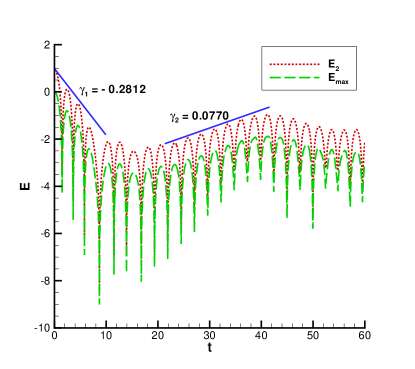
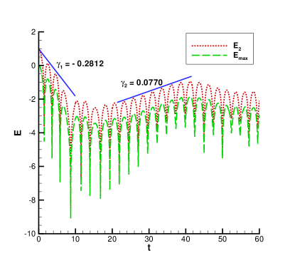
Figure 3.3: Strong Landau damping with the initial condition (3.9). Time evolution of the electric field in $L^{2}$ norm ($E_{2}$) and $L^{\infty}$ norm ($E_{max}$) (logarithmic value). Mesh: $N_{x}\times N_{v}=80\times 160$. Left: SL-WL; Right: RK-WL.

,
,

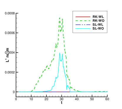
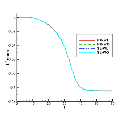
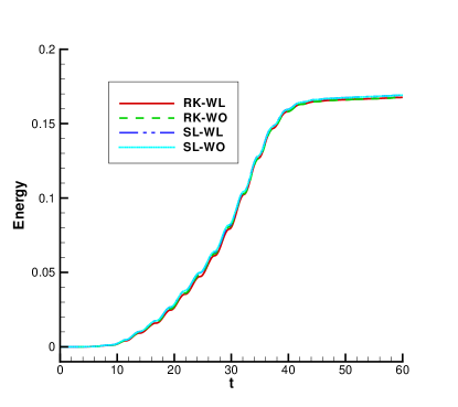
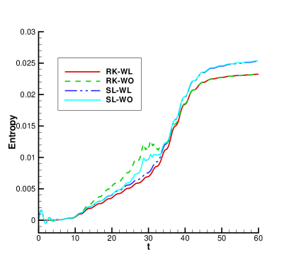
Figure 3.4: Strong Landau damping with the initial condition (3.9). Time evolution of the relative deviations of discrete $L^{1}$ norm (upper left), $L^{2}$ norm (upper right), kinetic energy (lower left) and entropy (lower right). $N_{x}\times N_{v}=80\times 160$.

Example 3.5.

(Two stream instability) We consider the symmetric two stream instability problem with the initial condition

$$f(0,x,v)=\frac{1}{2v_{th}\sqrt{2\pi}}\left[\exp\left(-\frac{(v-u)^{2}}{2v_{th}^{2}}\right)+\exp\left(-\frac{(v+u)^{2}}{2v_{th}^{2}}\right)\right](1+\alpha\cos(kx)),$$ (3.10)

where $\alpha=0.05$, $u=0.99$, $v_{th}=0.3$ and $k=\frac{2}{13}$. The time evolution of the electric field in $L^{2}$ norm and $L^{\infty}$ norm is plotted in Figure 3.5. The time evolution of the relative deviations of discrete $L^{1}$ norm, $L^{2}$ norm, kinetic energy and entropy are reported in Figures 3.6. The MPP flux limiters play a very good role on the $L^{1}$ norm, with very less effect on other discrete properties.

Similarly, the two stream instability problem with an unstable initial distribution function

$$f(0,x,v)=\frac{2}{7\sqrt{2\pi}}(1+5v^{2})(1+\alpha((\cos(2kx)+\cos(3kx))/1.2+\cos(kx))\exp(-\frac{v^{2}}{2}),$$ (3.11)

where $\alpha=0.01$ and $k=0.5$, has very similar results with and without limiters. We omit them to save some space.

,

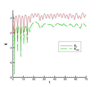
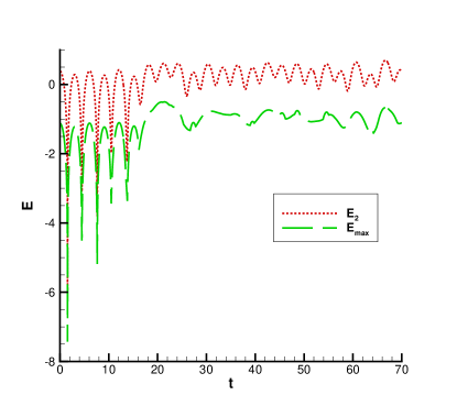
Figure 3.5: Symmetric two stream instability with the initial condition (3.10). Time evolution of the electric field in $L^{2}$ norm ($E_{2}$) and $L^{\infty}$ norm ($E_{max}$) (logarithmic value). $N_{x}\times N_{v}=80\times 160$. Left: SL-WL; Right: RK-WL.

,
,

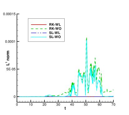
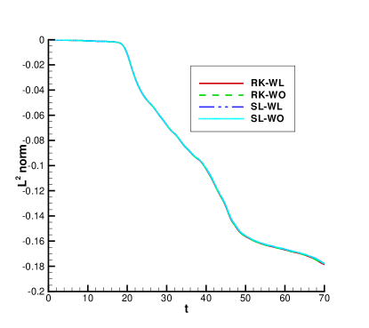
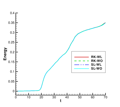
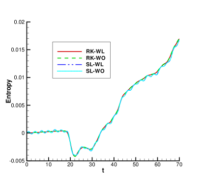
Figure 3.6: Symmetric two stream instability with the initial condition (3.10). Time evolution of the relative deviations of discrete $L^{1}$ norm (upper left), $L^{2}$ norm (upper right), kinetic energy (lower left) and entropy (lower right). $N_{x}\times N_{v}=80\times 160$.

Example 3.6.

(Bump-on-tail instability) We consider an unstable bump-on-tail problem with the initial distribution as

$$f(0,x,v)=f_{b.o.t}(v)(1+\alpha\cos(kx)),$$ (3.12)

where the bump-on-tail distribution is

$$f_{b.o.t}(v)=\frac{n_{p}}{\sqrt{2\pi}}\exp(-\frac{v^{2}}{2})+\frac{n_{b}}{\sqrt{2\pi}}\exp(-\frac{(v-v_{b})^{2}}{2v_{t}^{2}}).$$ (3.13)

The parameters are chosen to be $n_{p}=0.9$, $n_{b}=0.2$, $v_{b}=4.5$, $v_{t}=0.5$, $\alpha=0.04$, $k=0.3$. The computational domain is $[0,\frac{2\pi}{k}]\times[-8,8]$. We first show the time evolution of the $L^{\infty}$ norm for the electric field $E$ in Fig. 3.7. In Fig. 3.8, we display the relative deviations of discrete $L^{1}$ norm, $L^{2}$ norm, kinetic energy and entropy for the distribution function $f$ with and without limiters. Clearly we can observe that without limiters the $L^{1}$ norm is around $10^{-5}$, which indicates negative numerical values of $f$, while with limiters the $L^{1}$ norm is around machine error. The contour of the phase space for $f$ with and without limiters are also presented in Fig. 3.9. The results match those in [2] and slight difference can be seen between with and without limiters.

Figure 3.7: Bump-on-tail problem with initial condition (3.12). Time evolution of the electric field in the $L^{\infty}$ norm $E_{max}$. Mesh: $N_{x}\times N_{v}=256\times 256$.

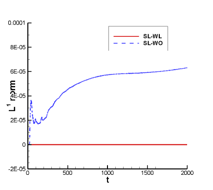
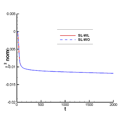
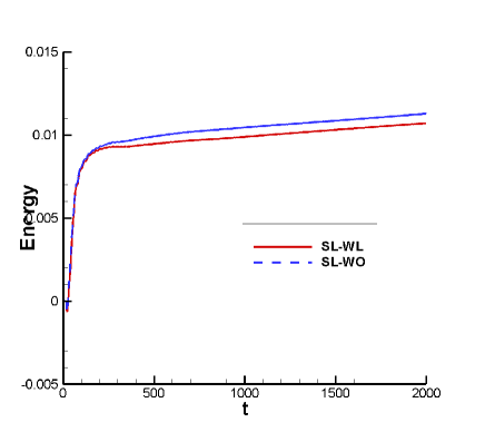
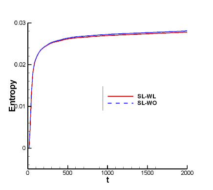
Figure 3.8: Bump-on-tail problem with initial condition (3.12). Time evolution of the relative deviations of discrete $L^{1}$ norm, $L^{2}$ norm, kinetic energy and entropy for the distribution functions $f$. Mesh: $N_{x}\times N_{v}=256\times 256$.

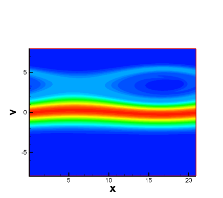
Figure 3.9: Bump-on-tail problem with initial condition (3.12). Contour of phase space for $f$ at $t=500$. 37 equally space contour lines within the range $[0,0.36]$. Mesh: $N_{x}\times N_{v}=256\times 256$. Left: with limiters; Right: without limiters.

Example 3.7.

(KEEN Wave) We consider the KEEN waves (kinetic electrostatic electron nonlinear waves) with the Vlasov equation

$$\partial_{t}f+v\cdot\nabla_{x}f+(E(t,x)-E_{ext})\cdot\nabla_{v}f=0,$$ (3.14)

where $E_{ext}=A_{d}(t)\sin(kx-\omega t)$ is the external field with $\omega=0.37$. $A_{d}(t)$ is a temporal envelope that is ramped up to a plateau and then ramped down to zero. Two external fields

$$A_{d}^{J}(t)=\begin{cases}A_{m}\sin(t\pi/100)\quad&0<t<50,\\ A_{m}\quad&50\leq t<150,\\ A_{m}\cos((t-150)\pi/100)\quad&150\leq t<200,\\ 0\quad&200\leq t<T,\end{cases}$$ (3.15)

with $A_{m}=0.052$ [21], and

$$A_{d}^{A}(t)=\begin{cases}A_{m}\frac{1}{1+e^{-40(t-10)}}\quad&0<t<60,\\ A_{m}\big{(}1-\frac{1}{1+e^{-40(t-110)}})\quad&60\leq t<T,\end{cases}$$ (3.16)

with $A_{m}=0.4$ [1] are considered. The system is initialized to be a Maxwellian $f(0,x,v)=1/\sqrt{2\pi}e^{-v^{2}/2}$. For both cases, the computational domain is taken to be $[0,2\pi/k]\times[-8,8]$, with $k=0.26$. We take the same mesh $N_{x}\times N_{v}=200\times 400$ as in [9], and consider the $n$th Log Fourier mode for the electric field $E(t,x)$ to be

$$logFM_{n}(t)=log_{10}\left(\frac{1}{L}\sqrt{\left|\int_{0}^{L}E(t,x)\sin(knx)dx\right|^{2}+\left|\int_{0}^{L}E(t,x)\cos(knx)dx\right|^{2}}\right).$$ (3.17)

We consider the SL method with and without limiter for this example. The first four Fourier modes are plotted in Figure 3.10 for the drive $A_{d}^{J}$. The time evolution of the relative deviations of discrete $L^{1}$ norm is around machine error for the solution even without limiter, little difference can be seen if with limiter, we omit the figures here to save space. The phase space contours for the drive $A_{d}^{A}$ at $t=15s,60s,120s,300s$ are plotted in Figure 3.11. We show the time evolution of the relative deviations of discrete $L^{1}$ norm and the first four Fourier modes for the drive $A_{d}^{A}$ in Figure 3.12. For this case, the $L^{1}$ norm has been significantly improved if with limiter.

,

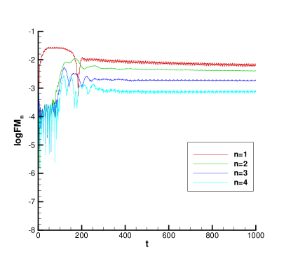
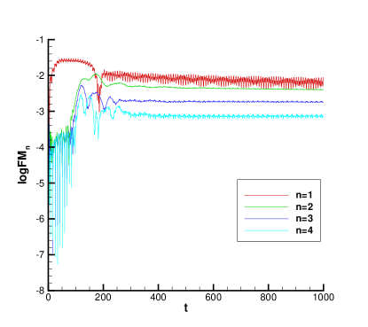
Figure 3.10: KEEN wave (3.14) with the drive $A_{d}^{J}$ (3.15). The first four Log Fourier Modes, n=1, 2, 3, 4 from top to bottom. Mesh: $N_{x}\times N_{v}=200\times 400$. Left: with limiter; Right: without limiter.

(a) t=15s

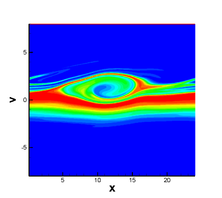
(b) t=60s

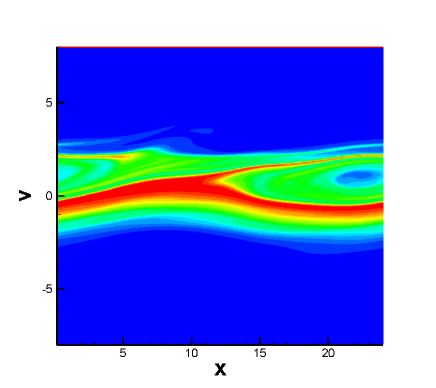
(c) t=120s

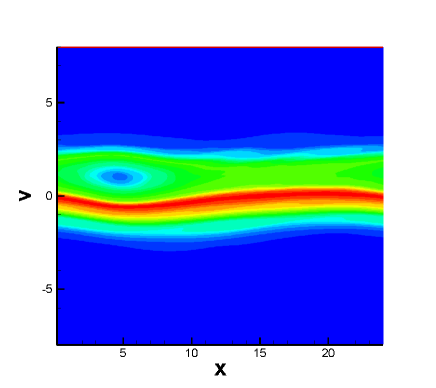
(d) t=300s

Figure 3.11: Phase space contour for the KEEN wave (3.14) with the drive $A_{d}^{A}$ (3.16). Mesh: $N_{x}\times N_{v}=200\times 400$.

,
,

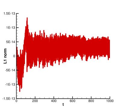
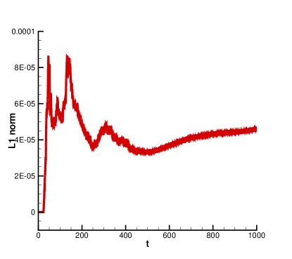
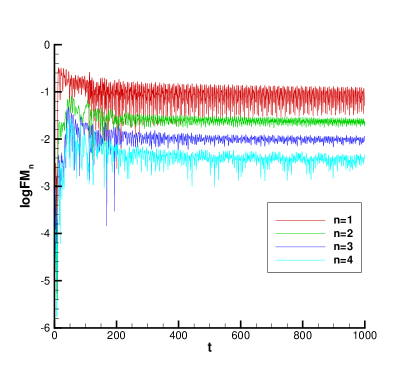
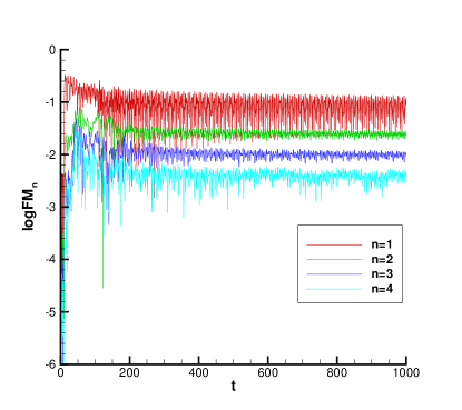
Figure 3.12: KEEN wave (3.14) with the drive $A_{d}^{A}$ (3.16). Time evolution of the relative deviations of discrete $L^{1}$ norm (Top) and the first four Log Fourier Modes (Bottom), n=1, 2, 3, 4 from top to bottom. Mesh: $N_{x}\times N_{v}=200\times 400$. Left: with limiter; Right: without limiter.

Example 3.8.

Now we consider a 1D Vlasov-Poisson system with two species of electrons and ions [2]. The electrons and ions have opposite charges of equal magnitude and mass ratio $m_{i}/m_{e}=M_{r}$. The Vlasov equations for electrons and ions are

$$\partial_{t}f_{e}+v\partial_{x}f_{e}-E(t,x)\partial_{v}f_{e}=0,$$ (3.18)

$$\partial_{t}f_{i}+v\partial_{x}f_{i}+\frac{E(t,x)}{M_{r}}\partial_{v}f_{i}=0,$$ (3.19)

where $E(t,x)$ is the electric field. The Poisson equation is taken to be

$$E(t,x)=-\nabla_{x}\phi(t,x),\qquad-\Delta_{x}\phi(t,x)=\int(f_{i}-f_{e})dv.$$ (3.20)

We study the ion-acoustic turbulence problem. The problem is the onset and saturation of the ion-acoustic instability. We take $M_{r}=1000$ and the initial ion distribution function is defined to be

$$f_{i}(0,x,v)=\Big{(}\frac{M_{r}}{2\pi}\Big{)}^{1/2}\exp\Big{(}-\frac{M_{r}}{2}v^{2}\Big{)}.$$ (3.21)

The electrons are a drifting Maxwellian and the initial distribution function is defined as

$$f_{e}(0,x,v)=(1+a(x))\frac{1}{\sqrt{2\pi}}\exp\Big{(}-\frac{1}{2}(v-U_{e})^{2}\Big{)},$$ (3.22)

where $U_{e}=-2$ and

$$a(x)= 0.01\big{(}\sin(x)+\sin(0.5x)+\sin(0.1x)+\sin(0.15x)+\sin(0.2x)$$

$$+\cos(0.25x)+\cos(0.3x)+\cos(0.35x)\big{)}.$$

The computational domain is $[0,\frac{2\pi}{0.05}]\times[-8,8]$. In Fig. 3.13, we show the difference of the ion and electron fluid speeds $u_{i}-u_{e}$, which indicates the momentum transfer from electrons to ions. We can see the decay rate agrees with the results in [2]. We also show the evoluntion of $L^{1}$ norms for the distribution functions $f_{e}$ and $f_{i}$ of both electrons and ions in Fig. 3.14. We can see the MPP limiters can effectively control the $L^{1}$ norms to machine error. The phase space for $f_{e}$ with and without limiters are displayed in Fig. 3.15, we can find that the result with limiters has more clear fine structures than the one without limiters.

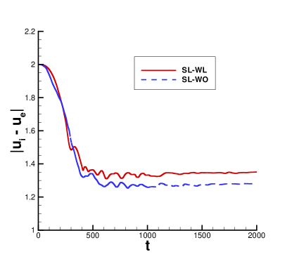
Figure 3.13: Ion-acoustic turbulence problem (3.19) and (3.18) with initial conditions (3.21) and (3.22). Time evolution of $|u_{i}-u_{e}|$. Mesh: $N_{x}\times N_{v}=256\times 256$.

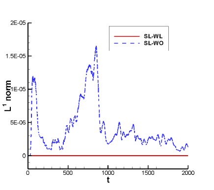
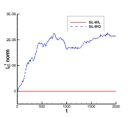
Figure 3.14: Ion-acoustic turbulence problem (3.19) and (3.18) with initial conditions (3.21) and (3.22). Time evolution of $L^{1}$ norms for the distribution functions $f_{e}$ (left) and $f_{i}$ (right). Mesh: $N_{x}\times N_{v}=256\times 256$.

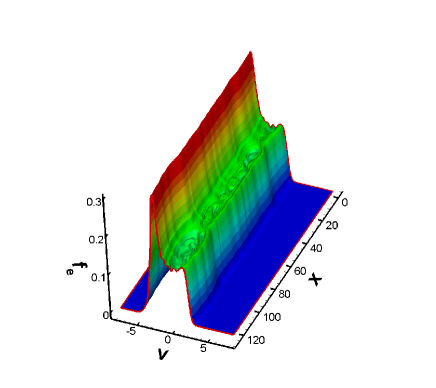
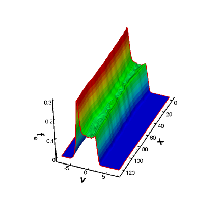
Figure 3.15: Ion-acoustic turbulence problem (3.19) and (3.18) with initial conditions (3.21) and (3.22). Surface of $f_{e}$ at $t=2000$. Mesh: $N_{x}\times N_{v}=256\times 256$. Left: with limiters; Right: without limiters.

4 Conclusion

In this paper, we generalized the parametrized MPP flux limiter to the semi-Lagrangian finite difference WENO scheme with application to the Vlasov-Poisson system. The MPP flux limiter preserves the maximum principle of the numerical solutions by the design, while maintaining the mass conservation and high order accuracy. Numerical studies demonstrate decent performance of the MPP flux limiter. In addition, the scheme can preserve the discrete $L^{1}$ norm up to the machine error.

Appendix A Appendix

Below, the first order numerical flux $h_{j+\frac{1}{2}}$ and the fifth order fluxes in (2.13) for the case of $|a|\Delta t\leq\Delta x$ are provided. For more details, see [28].

If $a>0$, let $\xi=a\frac{\Delta t}{\Delta x}$, the first order reconstructed flux would be

$$h_{i+\frac{1}{2}}=a\Delta tu^{n}_{i}.$$ (A.1)

The fifth order WENO reconstruction of $\mathcal{H}(x_{i+\frac{1}{2}})$ is a convex combination of three 3rd order fluxes, and is given by

$$\mathcal{H}(x_{i+\frac{1}{2}})=\omega_{1}\mathcal{H}^{(1)}(x_{i+\frac{1}{2}})+\omega_{2}\mathcal{H}^{(2)}(x_{i+\frac{1}{2}})+\omega_{3}\mathcal{H}^{(3)}(x_{i+\frac{1}{2}}),$$ (A.2)

where $\mathcal{H}^{(r)}(x_{i+\frac{1}{2}})$ is reconstructed from the following three potential stencils for $r=1,2,3$,

$$S_{1}=\{u^{n}_{i-2},u^{n}_{i-1},u^{n}_{i}\},\quad S_{2}=\{u^{n}_{i-1},u^{n}_{i},u^{n}_{i+1}\}\text{ and }S_{3}=\{u^{n}_{i},u^{n}_{i+1},u^{n}_{i+2}\}.$$

The reconstructed third order fluxes in (A.2) are

$$\mathcal{H}^{(1)}(x_{i+\frac{1}{2}}) = \Delta x\left((\frac{1}{6}\xi^{3}-\frac{1}{2}\xi^{2}+\frac{1}{3}\xi)u^{n}_{i-2}+(-\frac{1}{3}\xi^{3}+\frac{3}{2}\xi^{2}-\frac{7}{6}\xi)u^{n}_{i-1}+(\frac{1}{6}\xi^{3}-\xi^{2}+\frac{11}{6}\xi)u^{n}_{i}\right),$$

$$\mathcal{H}^{(2)}(x_{i+\frac{1}{2}}) = \Delta x\left((\frac{1}{6}\xi^{3}-\frac{1}{6}\xi)u^{n}_{i-1}+(-\frac{1}{3}\xi^{3}+\frac{1}{2}\xi^{2}+\frac{5}{6}\xi)u^{n}_{i}+(\frac{1}{6}\xi^{3}-\frac{1}{2}\xi^{2}+\frac{1}{3}\xi)u^{n}_{i+1}\right),$$ (A.4)

$$\mathcal{H}^{(3)}(x_{i+\frac{1}{2}}) = \Delta x\left((\frac{1}{6}\xi^{3}+\frac{1}{2}\xi^{2}+\frac{1}{3}\xi)u^{n}_{i}+(-\frac{1}{3}\xi^{3}-\frac{1}{2}\xi^{2}+\frac{5}{6}\xi)u^{n}_{i+1}+(\frac{1}{6}\xi^{3}-\frac{1}{6}\xi)u^{n}_{i+2}\right).$$ (A.5)

The linear weights $\gamma_{1}$, $\gamma_{2}$ and $\gamma_{3}$ are

$$\gamma_{1}=\frac{1}{10}+\frac{3}{20}\xi+\frac{1}{20}\xi^{2},\quad\gamma_{2}=\frac{3}{5}+\frac{1}{10}\xi-\frac{1}{10}\xi^{2},\quad\gamma_{3}=\frac{3}{10}-\frac{1}{4}{\xi}+\frac{1}{20}\xi^{2}.$$ (A.6)

The nonlinear weights $\omega_{1}$, $\omega_{2}$ and $\omega_{3}$ are computed by

$$\omega_{r}=\tilde{\omega}_{r}/\sum^{3}_{i=1}\tilde{\omega}_{i},\qquad\tilde{\omega}_{r}=\gamma_{r}/(\epsilon+\beta_{r})^{2},\quad r=1,2,3.$$ (A.7)

where $\epsilon$ is a small number to avoid the denominator becoming zero. In our numerical tests, we take $\epsilon=10^{-6}$. The smooth indicators $\beta_{1}$, $\beta_{2}$ and $\beta_{3}$ are

$$\beta_{1} = \frac{13}{12}(u^{n}_{i-2}-2u^{n}_{i-1}+u^{n}_{i})^{2}+\frac{1}{4}(u^{n}_{i-2}-4u^{n}_{i-1}+3u^{n}_{i})^{2},$$

$$\beta_{2} = \frac{13}{12}(u^{n}_{i-1}-2u^{n}_{i}+u^{n}_{i+1})^{2}+\frac{1}{4}(u^{n}_{i-1}-u^{n}_{i+1})^{2},$$

$$\beta_{3} = \frac{13}{12}(u^{n}_{i}-2u^{n}_{i+1}+u^{n}_{i+2})^{2}+\frac{1}{4}(3u^{n}_{i}-4u^{n}_{i+1}+u^{n}_{i+2})^{2}.$$

If $a<0$, let $\xi=|a|\frac{\Delta t}{\Delta x}$, the first order flux is

$$h_{i+\frac{1}{2}}=-|a|\Delta tu^{n}_{i+1}.$$ (A.8)

For the high order fluxes (A.2),

$$\mathcal{H}^{(1)}(x_{i+\frac{1}{2}}) = -\Delta x\left((\frac{1}{6}\xi^{3}-\frac{1}{6}\xi)u^{n}_{i-1}+(-\frac{1}{3}\xi^{3}+\frac{1}{2}\xi^{2}+\frac{5}{6}\xi)u^{n}_{i}+(\frac{1}{6}\xi^{3}-\frac{1}{2}\xi^{2}+\frac{1}{3}\xi)u^{n}_{i+1}\right),$$ (A.9)

$$\mathcal{H}^{(2)}(x_{i+\frac{1}{2}}) = -\Delta x\left((\frac{1}{6}\xi^{3}+\frac{1}{2}\xi^{2}+\frac{1}{3}\xi)u^{n}_{i}+(-\frac{1}{3}\xi^{3}-\frac{1}{2}\xi^{2}+\frac{5}{6}\xi)u^{n}_{i+1}+(\frac{1}{6}\xi^{3}-\frac{1}{6}\xi)u^{n}_{i+2}\right),$$ (A.10)

$$\mathcal{H}^{(3)}(x_{i+\frac{1}{2}}) = -\Delta x\left((\frac{1}{6}\xi^{3}-\xi^{2}+\frac{11}{6}\xi)u^{n}_{i+1}+(-\frac{1}{3}\xi^{3}+\frac{3}{2}\xi^{2}-\frac{7}{6}\xi)u^{n}_{i+2}+(\frac{1}{6}\xi^{3}-\frac{1}{2}\xi^{2}+\frac{1}{3}\xi)u^{n}_{i+3}\right),$$

with linear weights

$$\gamma_{1}=\frac{3}{10}-\frac{1}{4}{\xi}+\frac{1}{20}\xi^{2},\quad\gamma_{2}=\frac{3}{5}+\frac{1}{10}\xi-\frac{1}{10}\xi^{2},\quad\gamma_{3}=\frac{1}{10}+\frac{3}{20}\xi+\frac{1}{20}\xi^{2}.$$ (A.12)

The smooth indicators are

$$\beta_{1} = \frac{13}{12}(u^{n}_{i-1}-2u^{n}_{i}+u^{n}_{i+1})^{2}+\frac{1}{4}(u^{n}_{i-1}-4u^{n}_{i}+3u^{n}_{i+1})^{2},$$

$$\beta_{2} = \frac{13}{12}(u^{n}_{i}-2u^{n}_{i+1}+u^{n}_{i+2})^{2}+\frac{1}{4}(u^{n}_{i}-u^{n}_{i+2})^{2},$$

$$\beta_{3} = \frac{13}{12}(u^{n}_{i+1}-2u^{n}_{i+2}+u^{n}_{i+3})^{2}+\frac{1}{4}(3u^{n}_{i+1}-4u^{n}_{i+2}+u^{n}_{i+3})^{2}.$$

References

- [1] B. Afeyan, K. Won, V. Savchenko, T. Johnston, A. Ghizzo, and P. Bertrand, Kinetic electrostatic electron nonlinear (KEEN) waves and their interactions driven by the ponderomotive force of crossing laser beams, arXiv preprint arXiv:1210.8105, (2012).
- [2] T. Arber and R. Vann, A critical comparison of eulerian-grid-based vlasov solvers, Journal of computational physics, 180 (2002), pp. 339–357.
- [3] B. Ayuso, J. A. Carrillo, and C.-W. Shu, Discontinuous Galerkin methods for the one-dimensional Vlasov-Poisson system, Kinetic and Related Models, 4 (2011), pp. 955–989.
- [4] J. Barnes and P. Hut, A hierarchical O(N log N) force-calculation algorithm, Nature, (1986).
- [5] C. K. Birdsall and A. B. Langdon, Plasma Physics Via Computer Simulaition, CRC Press, 2005.
- [6] J. A. Carrillo and F. Vecil, Nonoscillatory interpolation methods applied to Vlasov-based models, SIAM Journal on Scientific Computing, 29 (2007), pp. 1179–1206.
- [7] C.-Z. Cheng and G. Knorr, The integration of the Vlasov equation in configuration space, Journal of Computational Physics, 22 (1976), pp. 330–351.
- [8] Y. Cheng, A. Christlieb, and X. Zhong, Energy-conserving discontinuous Galerkin methods for the Vlasov–Ampère system, Journal of Computational Physics, (in press).
- [9] Y. Cheng, I. M. Gamba, and P. J. Morrison, Study of conservation and recurrence of Runge–Kutta discontinuous Galerkin schemes for Vlasov–Poisson systems, Journal of Scientific Computing, (2012), pp. 1–31.
- [10] N. Crouseilles, M. Mehrenberger, and E. Sonnendrücker, Conservative semi-Lagrangian schemes for Vlasov equations, Journal of Computational Physics, 229 (2010), pp. 1927–1953.
- [11] B. A. de Dios, J. A. Carrillo, and C.-W. Shu, Discontinuous Galerkin methods for the multi-dimensional Vlasov–Poisson problem, Mathematical Models and Methods in Applied Sciences, 22 (2012).
- [12] J. W. Eastwood, Particle simulation methods in plasma physics, Computer Physics Communications, 43 (1986), pp. 89–106.
- [13] E. Evstatiev and B. Shadwick, Variational formulation of particle algorithms for kinetic plasma simulations, Journal of Computational Physics, 245 (2013), pp. 376–398.
- [14] E. Fijalkow, A numerical solution to the Vlasov equation, Computer Physics Communications, 116 (1999), pp. 319–328.
- [15] F. Filbet and E. Sonnendrücker, Comparison of Eulerian Vlasov solvers, Computer Physics Communications, 150 (2003), pp. 247–266.
- [16] F. Filbet, E. Sonnendrücker, and P. Bertrand, Conservative numerical schemes for the Vlasov equation, Journal of Computational Physics, 172 (2001), pp. 166–187.
- [17] W. Guo, R. D. Nair, and J.-M. Qiu, A conservative semi-Lagrangian discontinuous Galerkin scheme on the cubed-sphere, Monthly Weather Review, (2013).
- [18] W. Guo and J.-M. Qiu, Hybrid semi-Lagrangian finite element–finite difference methods for the Vlasov equation, Journal of Computational Physics, 234 (2013), pp. 108–132.
- [19] R. Heath, I. Gamba, P. Morrison, and C. Michler, A discontinuous Galerkin method for the Vlasov–Poisson system, Journal of Computational Physics, 231 (2012), pp. 1140–1174.
- [20] R. W. Hockney and J. W. Eastwood, Computer simulation using particles, CRC Press, 2010.
- [21] T. Johnston, Y. Tyshetskiy, A. Ghizzo, and P. Bertrand, Persistent subplasma-frequency kinetic electrostatic electron nonlinear waves, Physics of Plasmas, 16 (2009), p. 042105.
- [22] A. Klimas and W. Farrell, A splitting algorithm for Vlasov simulation with filamentation filtration, Journal of Computational Physics, 110 (1994), pp. 150–163.
- [23] A. J. Klimas, A method for overcoming the velocity space filamentation problem in collisionless plasma model solutions, Journal of Computational Physics, 68 (1987), pp. 202–226.
- [24] C. Liang and Z. Xu, Parametrized maximum principle preserving flux limiters for high order schemes solving multi-dimensional scalar hyperbolic conservation laws, Journal of Scientific Computing, (2013), pp. 1–20.
- [25] T. Nakamura and T. Yabe, Cubic interpolated propagation scheme for solving the hyper-dimensional Vlasov–Poisson equation in phase space, Computer Physics Communications, 120 (1999), pp. 122–154.
- [26] J.-M. Qiu and A. Christlieb, A conservative high order semi-Lagrangian WENO method for the Vlasov equation, Journal of Computational Physics, 229 (2010), pp. 1130–1149.
- [27] J.-M. Qiu and C.-W. Shu, Conservative high order semi-Lagrangian finite difference WENO methods for advection in incompressible flow, Journal of Computational Physics, 230 (2011), pp. 863–889.
- [28] , Conservative semi-Lagrangian finite difference WENO formulations with applications to the Vlasov equation, Communications in Computational Physics, 10 (2011), pp. 979–1000.
- [29] , Positivity preserving semi-Lagrangian discontinuous Galerkin formulation: theoretical analysis and application to the Vlasov–Poisson system, Journal of Computational Physics, 230 (2011), pp. 8386–8409.
- [30] J. A. Rossmanith and D. C. Seal, A positivity-preserving high-order semi-Lagrangian discontinuous Galerkin scheme for the Vlasov–Poisson equations, Journal of Computational Physics, 230 (2011), pp. 6203–6232.
- [31] E. Sonnendrücker, J. Roche, P. Bertrand, and A. Ghizzo, The semi-Lagrangian method for the numerical resolution of the Vlasov equation, Journal of Computational Physics, 149 (1999), pp. 201–220.
- [32] A. Staniforth and J. Côté, Semi-Lagrangian integration schemes for atmospheric models-a review, Monthly Weather Review, 119 (1991), pp. 2206–2223.
- [33] J. Strain, Semi-Lagrangian methods for level set equations, Journal of Computational Physics, 151 (1999), pp. 498–533.
- [34] T. Umeda, M. Ashour-Abdalla, and D. Schriver, Comparison of numerical interpolation schemes for one-dimensional electrostatic Vlasov code, Journal of Plasma Physics, 72 (2006), pp. 1057–1060.
- [35] T. Xiong, J.-M. Qiu, and Z. Xu, A parametrized maximum principle preserving flux limiter for finite difference RK-WENO schemes with applications in incompressible flows, Journal of Computational Physics, 252 (2013), pp. 310–331.
- [36] D. Xiu and G. E. Karniadakis, A semi-Lagrangian high-order method for Navier–Stokes equations, Journal of Computational Physics, 172 (2001), pp. 658–684.
- [37] Z. Xu, Parametrized maximum principle preserving flux limiters for high order scheme solving hyperbolic conservation laws: one-dimensional scalar problem, Mathematics of Computation, (in press).
- [38] S. Zaki, T. Boyd, and L. Gardner, A finite element code for the simulation of one-dimensional Vlasov plasmas. II. Applications, Journal of Computational Physics, 79 (1988), pp. 200–208.
- [39] S. Zaki, L. Gardner, and T. Boyd, A finite element code for the simulation of one-dimensional Vlasov plasmas. I. Theory, Journal of Computational Physics, 79 (1988), pp. 184–199.
- [40] X. Zhang and C. Shu, On maximum-principle-satisfying high order schemes for scalar conservation laws, Journal of Computational Physics, 229 (2010), pp. 3091–3120.
- [41] , Maximum-principle-satisfying and positivity-preserving high-order schemes for conservation laws: survey and new developments, Proceedings of the Royal Society A: Mathematical, Physical and Engineering Science, 467 (2011), pp. 2752–2776.
- [42] T. Zhou, Y. Guo, and C.-W. Shu, Numerical study on Landau damping, Physica D: Nonlinear Phenomena, 157 (2001), pp. 322–333.