Theoretical Constraints on Additional Higgs Bosons in Light of the 126 GeV Higgs

Abstract

We present a sum rule for Higgs fields in general representations under $SU(2)_{L}\times U(1)_{Y}$ that follows from the connection between the Higgs couplings and the mechanism that gives the electroweak bosons their masses, and at the same time restricts these couplings. Sum rules that follow from perturbative unitarity will require us to include singly and doubly charged Higgses in our analysis. We examine the consequences of these sum rules for Higgs phenomenology in both model independent and model specific ways. The relation between our sum rules and other works, based on dispersion relations, is also clarified.

I Introduction

The properties of the narrow resonance that has been discovered at the LHC is fit well by the Standard Model’s (SM’s) Higgs particle hypothesis. With the measured mass as input, the production rate and decay branching fractions are precisely predicted in the SM and compare well with the experiments.

In this note we ask a simple question: is it theoretically possible to have additional Higgs-like particles? We are interested in additional scalars that may have a mass different from 126 GeV but with similar production cross section and similar decay width into $\gamma\gamma$ and $WW$ final states. Alternatively one can ask, if such a particle (or particles) exist, what are the constraints on their properties? Are there model independent constraints?

The question may be more than academic. CMS has made public a note CMS-PAS-HIG-13-016 that points to a hint of a resonance at about 136 GeV observed in the $\gamma\gamma$ channel, which is produced both by gluon fusion (ggF) and vector boson fusion (VBF), with signal strength close to unity for both. Below we refer to the additional resonance as the $h^{\prime}$. Moreover, ATLAS and CMS claim to rule out heavier Higgs bosons through searches in the $WW$ and $ZZ$ channels ATLAS-CONF-2013-013 ; ATLAS-CONF-2013-067 ; CMS-PAS-HIG-12-024 ; CMS-PAS-HIG-13-002 ; CMS-PAS-HIG-13-003 ; CMS-PAS-HIG-13-008 ; CMS-PAS-HIG-13-014 . Naively combining these searches rules a neutral Higgs particle with mass in the range 128 GeV to 1000 GeV and SM interaction strength; see Appendix B. It is important to understand the generality of the assumptions for this limit, which we discuss in what follows.

Consider in some more detail the reported excess in the diphoton channel, seen in both ggF and VBF production modes. Following the procedure outlined in Ref Azatov:2012bz ; Azatov:2012qz we extract the production cross-section times branching ratio from the CMS exclusion limit:

$$\sigma_{ggF}\times BR(h^{\prime}\rightarrow\gamma\gamma) =0.036\pm 0.013\text{ pb},$$ (1)

$$\sigma_{VBF+Vh^{\prime}}\times BR(h^{\prime}\rightarrow\gamma\gamma) =0.007\pm 0.003\text{ pb}.$$

Dividing these cross sections by the SM prediction for a Higgs boson with $m_{h^{\prime}}=136.5$ GeV yields signal strengths, $\mu\equiv(\sigma\times\text{Br})/(\sigma_{SM}\times\text{Br}_{SM})$, of $\mu_{ggF}=1.1\pm 0.4$ and $\mu_{VBF}=1.6\pm 0.7$ respectively. Let’s characterize the coupling of $h^{\prime}$ to vector bosons and fermions by

$$\mathcal{L}_{h^{\prime}}\supset\frac{2m_{W}^{2}}{v_{\text{EW}}}a_{h^{\prime}}W^{\mu}W_{\mu}h^{\prime}+\frac{m_{Z}^{2}}{v_{\text{EW}}}a_{h^{\prime}}Z^{\mu}Z_{\mu}h^{\prime}-\sum_{i}\frac{m_{f_{i}}}{v_{\text{EW}}}c_{f_{i}}^{\prime}\bar{f}_{i}f_{i}h^{\prime}$$ (2)

where $v_{\text{EW}}=(\sqrt{2}G_{F})^{-1/2}\approx 246~{}\text{GeV}$ is the electroweak VEV. We assume (approximate) custodial symmetry, hence the same couplings $a_{h^{\prime}}$ to $W$ and $Z$. See Sec. 3A for a discussion of the constraints electroweak precision data puts on custodial-violating theories.

The parameters in Eq. (2) can be estimated from these two measurements by performing a $\chi^{2}$ fit to the data. Since there are more parameters than measurements, there should be at least one set of parameters that exactly reproduces the measurements. We assume that $h^{\prime}$ can only decay to SM particles, and that $\left|c_{f\neq t}^{\prime}\right|\leq 3$. The couplings we are most interested in are $a_{h^{\prime}}$ and $c_{t}^{\prime}$, so we project the allowed parameter space onto the $a_{h^{\prime}}-c_{t}^{\prime}$ plane. Note that we are not performing a goodness-of-fit test, but are simply trying to estimate parameters. The result is shown in Fig. 1. The green and yellow regions correspond to $\chi^{2}\leq 2.30$ and $6.18$, hence are compatible with the CMS measurements at the 68% and 95% confidence levels (CL), respectively.

Figure 1: Model independent analysis of the $h^{\prime}$ couplings. The green and yellow regions are compatible with the CMS hint of a 136 GeV Higgs resonance at 68% and 95% CL, respectively.

Alternatively, it is instructive to see what happens when an ansatz is made for the other parameters in the model. In Fig. 2a, the couplings of $h^{\prime}$ to fermions other than the top-quark are fixed to a common value. The dotted, solid, and dashed contours correspond to $c^{\prime}_{f\neq t}=\{0,1,2\}$ respectively, while in Fig. 2b, the signal strength modifier for fermions is assumed to be universal. The latter is an interesting case because there is a class of models, which we discuss in depth below, where there is a single common $c_{f}^{\prime}$ for all fermions.

(a)

(b)

Figure 2: The preferred values of $(a_{h^{\prime}},c^{\prime}_{t})$ for interpreting the bump in the CMS data as a second Higgs boson. The regions of parameter space that are allowed at 68% and 95% CL are shown in green and yellow, respectively. In Fig. 2a, the couplings of $h^{\prime}$ to fermions other than the top-quark are fixed to a common value. The dotted, solid, and dashed contours correspond to $c^{\prime}_{f\neq t}=\{0,1,2\}$ respectively. In Fig. 2b, the signal strength modifier for fermions is assumed to be universal.

We see that CMS measurements prefer sizable coupling of $h^{\prime}$ to both the top and the vector-bosons. The question we posed above can be stated more specifically: how much of the allowed region in Fig. 1 is compatible with the established properties of the 126 GeV Higgs resonance? We hasten to indicate that we address this question in generality, not just as it may pertain to a putative state at 136 GeV (but we do use the 136 GeV CMS data as an instructive example).

What precisely do we mean by “Higgs-like” particles? What makes a Higgs-like particle, or Higgs for short, special is its tri-linear coupling to electroweak vector bosons, say $hW^{+}W^{-}$ or $hZZ$. Indeed, in a gauge theory all fields, $\psi$, except the Higgs, have couplings to gauge bosons, $A$, with the field appearing quadratically, $\psi^{2}A$ or $\psi^{2}A^{2}$. Hence a unique characteristic of Higgs particles is that they can be produced in $s$-channel vector boson fusion, and can decay into pairs of vector bosons. This generalized definition of Higgs particle includes, of course, singly and doubly charged particles in addition to the more familiar neutral (CP-even) Higgs. In fact, considerations of perturbative unitarity will require that we include singly and doubly charged Higgs in our analysis.

We will derive a number of sum rules that will restrict the couplings of the Higgs particles. The sum rules are model independent, but derived only at tree level. For each sum rule we derive we will show in explicit examples how they are saturated. We will see, model independently, that not all the allowed region in Fig. 1 is compatible with the established properties of the 126 GeV Higgs resonance. We will also see that the region in Fig. 1 compatible with several specific models of the $h^{\prime}$ is further restricted.

Sum rules for Higgs particles have been considered before. There is a vast literature on 2HDM models, recasting explicit results as sum rules, see e.g. Grzadkowski:1999wj ; Ginzburg:2004vp ; Celis:2013rcs ; Celis:2013ixa for an incomplete list. Sum rules for the couplings of arbitrary number of Higgses in general representations of the electroweak group were first derived by Gunion, Haber, and Wudka using perturbative unitarity arguments in Gunion:1990kf . To make the presentation self-contained, we review below the derivation of these sum rules. In addition, we present bounds on combinations of masses and couplings of the Higgs particles, that to the best of our knowledge have not been considered for general Higgs sectors before. These perturbative unitarity mass bounds are the multi-Hiiggs generalization of the celebrated result by Lee, Quigg and Thacker Lee:1977eg that placed an upper bound on the higgs mass of $\sim$700 GeV. In Ref. Distler:2006if a twice subtracted dispersion relation for longitudinal $WW$ scattering was obtained and applied to Higgsless models. In Ref. Low:2009di ; Falkowski:2012vh ; Urbano:2013aoa , a similar relation was given for a model with a single Higgs particle with non-standard couplings. In particular, it was shown that the couplings of the light Higgs to a $W$ pair obeys the following simple dispersion relation

$$1-a^{2}_{h}=\frac{v^{2}}{\pi}\int^{\infty}_{0}\frac{ds}{s}\left(\sigma_{+-}(s)-\sigma_{++}(s)\right)~{},$$ (3)

where $\sigma_{+-}$ denotes the cross section for a longitudinal $W$ pair annihilation, $W^{L+}W^{L-}\to\textit{anything}$, and similarly for $\sigma_{++}$. Moreover, it was noticed in Ref. Low:2009di ; Falkowski:2012vh that the last relation implies that enhanced Higgs $\to WW$ couplings require doubly charged states (that couple to vector bosons) be present in the theory.

We will generalize (3) to a multi-Higgs case below. This dispersion relation holds under the assumption of unitarity of the full UV theory (supplemented by a more technical assumption that the Froissart bound is sufficiently unsaturated). While (3) is true to all orders in the loop expansion and for nonperturbative theories as well as perturbative ones, in what follows we will be exclusively interested in the tree-level amplitudes in perturbative theories with definite UV field content. Our tree-level sum rules will then guarantee that the assumption of (perturbative) unitarity under which (3) holds is satisfied at order $\hbar^{0}$. We discuss how exactly our sum rules are consistent with (3) in detail in Sec. VII and App. C.

The paper is organized as follows. In Sec. II we present a simple sum rule for multi-Higgs doublet models that follows from the connection between the Higgs couplings and the mechanism that gives the electroweak bosons their masses, and we generalize this to models with Higgs fields in other representations of $SU(2)_{L}\times U(1)_{Y}$ in Sec. III. These sum rules are model dependent, so in Sec. IV we turn to sum rules that follow from perturbative unitarity. We examine the consequences of these sum rules on the allowed region in Fig. 1 in Sec. V. We then study in some detail the phenomenology of some specific models in Sec. VI. Finally we study the relation between our sum rules and other work, based on dispersion relations in Sec. VII and offer some concluding remarks in Sec. VIII. To make the paper easily accessible, we list the physical Higgses couplings in App. A. We collect the Higgs data used in our analysis in App. B. App. C is devoted to detailed derivation of the dispersion relation.

II multi-Higgs Doublet model

The CMS note points out that the $h^{\prime}$ is incompatible with a two Higgs doublet model (2HDM) hypothesis (see, e.g., Grinstein:2013npa ; Barbieri:2013hxa ; Barbieri:2013nka and references therein for a recent general analysis of Type-II 2HDM and (N)MSSM Higgs sectors). The reason is this. Since both the 126 GeV and 136 GeV states couple with similar strength to $WW$, we can immediately discount the CP-odd neutral Higgs as one of these states. Assuming the light CP-even neutral Higgs is the particle observed at 126 GeV, fits of Higgs data to the 2HDM assumption give $\alpha+\beta\approx\pm\pi/2$, where $\alpha$ is the mixing angle between CP-even neutral Higgs mass eigenstates and $\tan\beta=v_{1}/v_{2}$ is the ratio of the vacuum expectation values (VEV) of the two doublets. The ratio of the coupling of the heavier Higgs to $WW$ to that of the lighter Higgs is $\cot(\alpha+\beta)$, so the fit gives a very suppressed $h^{\prime}$ to $W^{+}W^{-}$ coupling.

This observation is readily generalized to models with any number of Higgs doublets. Consider a model with $N$ Higgs doublets, $H_{i}$, all with $Y=\tfrac{1}{2}$, with VEV $v_{i}/\sqrt{2}$ and CP even neutral scalar $\tilde{h}_{i}$. The kinetic energy terms of these doublets give the $W$-mass and the couplings of the $\tilde{h}_{i}$ to $W^{+}W^{-}$:

$$\mathcal{L}=\cdots+\tfrac{1}{4}g^{2}W^{+}_{\mu}W^{-}_{\nu}\eta^{\mu\nu}\sum_{i=1}^{N}(v_{i}+\tilde{h}_{i})^{2}.$$ (4)

This can be interpreted as follows. The vector $\tfrac{1}{2}g^{2}(v_{1},\ldots,v_{N})\equiv gM_{W}\vec{\tilde{a}}=gM_{W}(\tilde{a}_{1},\ldots,\tilde{a}_{N})$ characterizes the couplings of the fields $\vec{\tilde{h}}=(\tilde{h}_{1},\ldots,\tilde{h}_{N})$ to $W^{+}W^{-}$, and the norm of the vector is fixed, $|\vec{\tilde{a}}|^{2}=1$. The fields in $\vec{\tilde{h}}$ do not in general correspond to mass eigenstates. An orthogonal rotation $\vec{\tilde{h}}=R\vec{h}$ brings the mass matrix to diagonal form. The mass eigenstates couple to $WW$ with strength $\vec{a}=R^{T}\vec{\tilde{a}}$. Since $R$ is orthogonal $|\vec{\tilde{a}}|^{2}=1$ implies $|\vec{a}|^{2}=1$. Without loss of generality we take $h_{1}$ to correspond to the 126 GeV observed resonance. Then

$$\sum_{i>1}a_{i}^{2}=1-a_{1}^{2}\,.$$ (5)

That is, the CP-even neutral Higgs resonances other than $h_{1}$ (the observed 126 GeV one) can couple to $WW$ only to the extent that the coupling of $h_{1}$ to $WW$ differs form that of Higgs in the (one Higgs doublet) SM.

III Generalizations

The results of the previous section can be generalized to the case of Higgs fields in any non-trivial representation of $SU(2)$. This may seem as only of academic interest since electroweak precision data (EWPD) places stringent constraints on the VEV of non-doublet representations. But there are exceptions, like the model of Georgi and Machacek Georgi:1985nv and models with isospin-3 fields Kanemura:2013mc . We carry out the analysis in general, and return below to considerations of EWPD.

In the case of arbitrary representations, Eq. (4) is replaced by

$$\mathcal{L}=\cdots+\tfrac{1}{4}g^{2}W^{+}_{\mu}W^{-}_{\nu}\eta^{\mu\nu}\sum_{i=1}^{N}C_{i}(v_{i}+\tilde{h}_{i})^{2},$$ (6)

where we assume $\tilde{h}_{i}$ is the CP-even neutral scalar from the $(2n_{i}+1)$-dimensional representation, with the third component of isospin given by $m_{i}$, so that

$$C_{i}=C(n_{i},m_{i})=2[n_{i}(n_{i}+1)-m_{i}^{2}].$$ (7)

The couplings of $\tilde{h}_{i}$ are now characterized by $\vec{\tilde{a}}=\tfrac{g}{2M_{W}}(C_{1}v_{1},\ldots,C_{N}v_{N})$ and those of mass eigenstates by $\vec{a}=R^{T}\vec{\tilde{a}}$, with $R^{T}R=1$. The constraint

$$\sum_{i=1}^{N}\frac{\tilde{a}_{i}^{2}}{C_{i}}=1,$$ (8)

is an ellipse in $\vec{\tilde{a}}$ space. Rotating to $\vec{a}$ space, this remains an ellipse. Now suppose one of the couplings in $\vec{a}$ has been measured. Without loss of generality we take this to be the first component, $a_{1}$. For $a_{1}$ sufficiently close to $1$, the least constraining case is when the rotation $R$ makes $a_{1}$ line up with the semi-major axis. Consider, for example, the $N=2$ case with $C_{1}=1$ and $C_{2}>1$. Then we must have

$$a_{2}^{2}=1-\frac{a_{1}^{2}}{C_{2}}~{}.$$ (9)

More generally, the constraint on the coupling of the mass eigenstates to $WW$ takes the form

$$a^{T}R^{T}C^{-1}Ra=1,$$ (10)

where $C$ is the diagonal matrix of the $C_{i}$ and we have used vector notation (with $a=\vec{a}$). This in principle alleviates constraints on the magnitude of couplings of extra neutral Higgs bosons to $W$ and $Z$.

While the rotation to the mass eigenstate may greatly relax the constraint on the coupling of the second Higgs, the coupling of the first Higgs resonance to fermions is correspondingly reduced. Only isospin-$\tfrac{1}{2}$ states can couple directly to fermions. If only $H_{1}$ is in the doublet representation then the coupling to fermions is through

$$\mathcal{L}_{f}=\tilde{H}_{1}\bar{q}_{L}\lambda_{U}u_{R}+H_{1}\bar{q}_{L}\lambda_{D}d_{R}+H_{1}\bar{\ell}_{L}\lambda_{E}e_{R},$$ (11)

where $\tilde{H}_{1}=i\sigma^{2}H_{1}^{*}$ and $\lambda_{U,D,E}$ are the matrices of Yukawa couplings. Expanding this about the vacuum and retaining only the couplings of the neutral Higgs mass eigenstates one obtains

$$\mathcal{L}_{f}=\frac{1}{v_{1}}R_{1i}h_{i}\left(\bar{u}m_{U}u+\bar{d}m_{D}d+\bar{e}m_{E}e\right)~{},$$ (12)

where $m_{U,D,E}$ are the mass matrices. Orthogonality of $R$ implies $\sum_{i>1}R^{2}_{1i}=1-R^{2}_{11}$, limiting the extent to which the remaining Higgs resonances couple to fermions. Returning to the simple example above, in the extreme case that the doublet field $C_{1}=1$ is maximally rotated with a non-doublet, $C_{2}>1$ as given by Eq. (9), one has $R_{11}=0$ and $R_{12}=1$ and only one resonance couples to fermions.

III.1 Electroweak constraints

Precision measurements of electroweak parameters place stringent constraints on the possibility of VEV for Higgs multiplets other than the doublet and the septet (isospin-3). The deviation of the $\rho$ parameter from unity (or, equivalently, the $T$-parameter) constraints the VEV of the multiplets at tree level:

$$\delta\rho=\frac{M_{W}^{2}-M_{3}^{2}}{M_{3}^{2}},$$ (13)

where $M_{W}$ is the $W^{\pm}$ mass and $M_{3}=M_{Z}\cos\theta_{W}$ that of the neutral component of the $SU(2)$ vector boson multiplet. At tree level, in the case of $N$ multiplets $H_{i}$, $i=1,\ldots,N$, with $H_{i}$ in the $(2n_{i}+1)$-dimensional representation of $SU(2)$ with VEV $v_{i}/\sqrt{2}$ in the $T_{3}=m_{i}$ component (and hypercharge of $Y(H_{i})=-m_{i}$), we obtain

$$\delta\rho=\frac{\sum_{i}v_{i}^{2}[n_{i}(n_{i}+1)-3m_{i}^{2}]}{\sum_{i}2v_{i}^{2}m_{i}^{2}},$$ (14)

Note that for $gn_{i}\leq 4\pi$, a loose requirement for perturbation theory to hold, $n_{i}(n_{i}+1)-3m_{i}^{2}$ vanishes for $n_{i}=|m_{i}|=\frac{1}{2}$ or $n_{i}=3$, $|m_{i}|=2$ only (additional solutions are found for larger isospin, e.g., $n_{i}=48$, $|m_{i}|=28$ or $n_{i}=\tfrac{361}{2}$, $|m_{i}|=\tfrac{209}{2}$).

Quantum corrections due to additional Higgs bosons can be conveniently studied in terms of the oblique parameters, in particular the well-known $S$ and $T$. We do not attempt to study these corrections for arbitrary Higgs representation. The results largely depend on the exact form of the Higgs potential, that we leave unspecified in this work. We refer the readers to the literature for relevant studies. In the case of multi-Higgs doublets, these corrections are well known Grimus:2008nb ; see Barbieri:2013aza for a recent discussion. For the GM model, constraints from EWPD have been analyzed in Englert:2013zpa .

In the context of the doublet-septet model, the $S$ and $T$ parameters have only been studied in the special case where the charged Higgs spectrum is taken to be degenerate with the exception of one singly charged Higgs Hisano:2013sn .

IV Perturbative Unitarity

Perturbative unitarity of the SM has been famously used to place a bound of about 700 GeV on the Higgs mass. Lee, Quigg and Thacker (LQT) Lee:1977eg observed that the tree level partial wave amplitudes for longitudinally polarized $W^{+}W^{-}$ scattering grow with the Higgs mass, so that at large enough mass the amplitudes exceed the unitarity bound. They also pointed out that in the absence of the Higgs particle the $J=0,1$ partial wave amplitudes grow with the square of the center of mass energy $s$, but the exchange of the Higgs particle in the $s$- and $t$-channels cancels the linear growth with $s$ of these amplitudes.

IV.1 Sum rule for $W^{+}_{L}W^{-}_{L}\to W^{+}_{L}W^{-}_{L}$

Applying the LQT argument to the multi-Higgs doublet extension of the SM gives an alternate derivation of the sum rule (5). It is the statement that the couplings that appear in the $s$- and $t$- channel neutral Higgs exchange must add up to those of the SM contribution in order to cancel the linear growth with $s$ of the $J=0,1$ partial wave amplitudes.

This suggests a more general approach to the sum rule for any number of $N$ neutral resonances $h_{i}$ that couple to $W^{+}W^{-}$ with strength $a_{i}$, namely

$$\sum_{i=1}^{N}a_{i}^{2}\overset{?}{=}1.$$ (15)

The constraint (15) is stronger than the one in (8), which must hold in order to obtain the correct $W$ mass in a multi-Higgs model with at least one Higgs multiplet of isospin 1 or higher. And it is incorrect. In general there are additional contributions to the $W^{+}W^{-}$ scattering amplitude from $u$-channel exchange of a doubly charged component of the multiplet to which $h_{i}$ belongs.

(a)

Figure 3: $W^{+}W^{-}$ scattering in the presence of a generic Higgs sector. Diagrams a-c refer to the scattering in the Higgsless standard model, with $W^{3}$ collectively denoting the exchange of the $Z$ boson and the photon. The growth with the center of mass energy of these contributions can be cancelled by neutral (d, e) or doubly charged (f) Higgses.

To see that this is the case we compute the amplitude for longitudinal $W^{+}W^{-}$ scattering including contributions from a neutral Higgs with arbitrary coupling $gM_{W}a$ to $W^{+}W^{-}$ and of a doubly charged complex scalar with arbitrary coupling $gM_{W}b$ to $W^{+}W^{+}$ (plus hermitian conjugate). Only the $J=0$ and 1 partial wave amplitudes exhibit linear growth with $s$, and the coefficient of the term exhibiting linear growth is common to both amplitudes and proportional to

$$\kappa_{1}=4-3(M_{3}/M_{W})^{2}-a^{2}+4b^{2}.$$ (16)

Here, the first two terms come from the pure gauge sector, Fig. 3a-c. The second term arises when the exchanged neutral gauge boson is massive, Fig. 3b and  3c. The third term is the contribution of the neutral Higgs exchange in both $s$- and $t$-channels, Fig. 3d and  3e. The last term comes from the $u$-channel exchange of a doubly charged scalar, Fig. 3f. In Eq. (16) the terms $a^{2}$ and $b^{2}$ should be replaced by a sum over squares of couplings, $\sum a_{i}^{2}$ and $\sum_{r}b_{r}^{2}$, when more than one neutral or doubly charged states are present. The correct version of the sum rule in Eq. (15) reads

$$\sum_{i}a_{i}^{2}-4\sum_{r}b_{r}^{2}=4-3(M_{3}/M_{W})^{2}~{}.$$ (17)

Following LQT we can also obtain an upper limit on a combination of the masses $M^{0}_{i}$ and $M^{++}_{r}$ of the neutral and doubly charged Higgses. We quickly review the LQT computation. They consider (in the SM) first the limit $M_{h}\gg M_{W}\sim M_{Z}$ of the $J=0$ partial wave scattering amplitude for $W_{L}^{+}W_{L}^{-}\to W_{L}^{+}W_{L}^{-}$, followed by the large CM energy limit. They find the following expression for (the finite piece of) the $s$-wave scattering amplitude

$$a_{0}(W_{L}^{+}W_{L}^{-}\to W_{L}^{+}W_{L}^{-})\xrightarrow[s\gg M_{h}^{2}\gg M_{W}^{2}]{}-\frac{G_{F}M_{h}^{2}}{4\pi\sqrt{2}},$$ (18)

from which the condition $\big{|}a_{0}(W_{L}^{+}W_{L}^{-}\to W_{L}^{+}W_{L}^{-})\big{|}\leq 1$ gives $M_{h}^{2}\leq 4\pi\sqrt{2}/G_{F}$. LQT derive a slightly better bound by performing a coupled channel analysis including also $ZZ$, $Zh$ and $hh$ scattering.

Below we use a slightly more constraining condition that follows from unitarity, $\big{|}\text{Re}\big{[}a_{0}(W_{L}^{+}W_{L}^{-}\to W_{L}^{+}W_{L}^{-})\big{]}\big{|}\leq 1/2$. The same procedure gives, for the more general case considered here,

$$\sum_{i}(a_{i}M^{0}_{i})^{2}+2\sum_{r}(b_{r}M^{++}_{r})^{2}\leq\frac{2\pi\sqrt{2}}{G_{F}}\approx 0.5~{}\text{TeV}^{2}~{}.$$ (19)

To obtain this bound the limit of small $M_{W,Z}$ is taken first at constant Higgs masses, and only then the large $s$ limit is taken. The contribution of the $a_{1}\approx 1$, $M^{0}_{1}\approx 126$ GeV Higgs to the bound is negligible (which is consistent with the approximation of neglecting the similarly small masses $M_{W}$ and $M_{Z}$).

IV.1.1 Examples

For explicit examples, we first consider the simpler case of an $SU(2)$ gauge theory with a single Higgs field $\Phi$ with isospin $(2n+1)$. We assume the VEV of the field, $v/\sqrt{2}$, is in the $T^{3}=m$ component of the multiplet with hypercharge $Y=-m$. Let

$$\Phi-\langle\Phi\rangle=\sum_{k}\phi_{k}|k\rangle,$$ (20)

where $|k\rangle$ is a normalized $2n+1$ dimensional vector in isospin space, with $T^{3}|k\rangle=k|k\rangle$. Then the lagrangian contains a term

$$\mathcal{L}\supset\frac{g^{2}v}{\sqrt{2}}\eta^{\mu\nu}\left[A\left(W^{+}_{\mu}W^{+}_{\nu}\phi_{m-2}+W^{-}_{\mu}W^{-}_{\nu}\phi_{m-2}^{*}\right)+B\left(W^{+}_{\mu}W^{+}_{\nu}\phi_{m+2}^{*}+W^{-}_{\mu}W^{-}_{\nu}\phi_{m+2}\right)\right],$$ (21)

where

$$A=A(n,m) =\langle m|T^{+}T^{+}|m-2\rangle=\langle m-2|T^{-}T^{-}|m\rangle$$ (22)

$$=\frac{1}{2}\sqrt{\left[n(n+1)-(m-2)(m-1)\right]\left[n(n+1)-m(m-1)\right]}\,,$$

$$B=B(n,m) =A(n,m+2)=\langle m+2|T^{+}T^{+}|m\rangle=\langle m|T^{-}T^{-}|m+2\rangle$$

$$=\frac{1}{2}\sqrt{\left[n(n+1)-m(m+1)\right]\left[n(n+1)-(m+1)(m+2)\right]}\,.$$

Note that $A=0$ for $m=-n$ and $m=-n+1$, and $B=0$ for $m=n$ and $m=n-1$, so these coefficients automatically account for the absence of charged states with disallowed isospin components, i.e., $m=n+2$, $n+1$, $-n-1$ or $-n-2$. Of course, $A=B=0$ in the case $|m|=n=\tfrac{1}{2}$. Using $M_{W}^{2}=\tfrac{1}{4}g^{2}v^{2}C$ where $C=2[n(n+1)-m^{2}]$ as per Eq. (7), $M_{3}^{2}=g^{2}v^{2}m^{2}$, $a=\sqrt{C}$ from Eq. (6) and $\sum_{i}b_{i}^{2}=2(A^{2}+B^{2})/C$, one finds $\kappa_{1}=0$ in Eq. (16). Note that for all cases other than $n=\tfrac{1}{2}$ (the SM) and $n=1$ with $Y=0$ (the prototypical triplet Higgs model), the contribution of the doubly charged Higgs particle is crucial to insure perturbative unitarity at high energies. The generality of this result is remarkable. Note for example, that for integer $n$ with $Y=0$ the pattern of symmetry breaking is $SU(2)\to U(1)$ so that $W^{3}$ remains exactly massless. In this case the vanishing of $\kappa_{1}$ results from the cancellation of the first, third and fourth terms in Eq. (16). The second term is absent because $W^{3}$ is massless.

The bound on the masses in (19), assuming for simplicity that the two doubly charged states are mass-degenerate with masses $M^{++}$, gives

$$C(M^{0})^{2}+4\frac{A^{2}+B^{2}}{C}(M^{++})^{2}\leq 2\pi\sqrt{2}/G_{F}\approx 0.5~{}\text{TeV}^{2}.$$

For a concrete and pertinent example, take $n=3,m=2$; then $16(M^{0})^{2}+\tfrac{15}{2}(M^{++})^{2}\leq 0.5~{}\text{TeV}^{2}$. This is very constraining: it gives $M^{0}\leq 177$ GeV, $M^{++}\leq 259$ GeV, and if the masses are comparable, $M^{0}\approx M^{++}\leq 146$ GeV.

One can readily generalize above discussion to the realistic case with gauge group $SU(2)_{L}\times U(1)_{Y}$. Electric charge conservation requires the VEV in the electrically neutral component, $Q=T^{3}+Y=0$, fixing the hypercharge of the Higgs multiplet, $Y_{\phi}=-m$. This implies that the $Z$-boson, $Z=\cos\theta_{W}W^{3}-\sin\theta_{W}B$, has mass given by

$$M_{Z}=\sqrt{g^{2}+g^{\prime 2}}~{}mv=\frac{g}{\cos\theta_{W}}~{}mv~{}.$$ (23)

Here, $g$ and $g^{\prime}$ are the gauge couplings for $SU(2)_{L}$ and $U(1)_{Y}$ respectively, while the electroweak angle is defined in the standard way, $\cos\theta_{W}=g/\sqrt{g^{2}+g^{\prime 2}}$. The sum rule obtained by setting $\kappa_{1}$ in (16) to zero is automatic, provided one substitutes

$$M_{3}^{2}\to g^{2}m^{2}v^{2}=M^{2}_{Z}\cos^{2}\theta_{W}.$$ (24)

The latter substitution can be understood by noting that the only differences in the computation for longitudinal $W$ scattering through $Z$ exchange in a theory with $U(1)_{Y}$ come from different couplings and intermediate vector masses. One can show by a straightforward computation, that while the part of $W_{L}$ scattering amplitude that grows as $s^{2}$ cancels identically in the gauge sector, the linear piece is given as follows

$$\mathcal{M}_{lin} =-g^{2}s\bigg{[}\frac{3\cos\theta-1}{2M_{W}^{2}}+\cos^{2}\theta_{W}\left(\frac{\cos\theta M_{Z}^{2}}{4M_{W}^{2}}+\frac{M_{Z}^{2}~{}(3+\cos\theta)-16M_{W}^{2}\cos\theta}{8M^{4}_{W}}\right)$$

$$-\sin^{2}\theta_{W}\frac{2\cos\theta}{M^{2}_{W}}\bigg{]}=g^{2}s~{}(1+\cos\theta)~{}\frac{\textbullet 4M^{2}_{W}-3M^{2}_{Z}\cos^{2}\theta_{W}}{8M^{4}_{W}}~{}.$$ (25)

The first term in the first line corresponds to the contact interaction, the second and third terms, with coefficient $\cos^{2}\theta_{W}$ are the $s$-and $t$-channel $Z$ exchange, respectively, and the fourth term, proportional to $\sin^{2}\theta_{W}$, is from photon exchange.

Adding the contributions of the neutral and doubly charged Higgs bosons leads to the following sum rule in a $SU(2)_{L}\times U(1)_{Y}$ - invariant theory with a generic Higgs sector

$$4-3\frac{M_{Z}^{2}\cos^{2}\theta_{W}}{M_{W}^{2}}-a^{2}+4b^{2}=\left(4-\frac{3}{1+\delta\rho}\right)-a^{2}+4b^{2}=0~{},$$ (26)

where $\delta\rho\equiv\frac{M^{2}_{W}}{M^{2}_{Z}\cos^{2}\theta_{W}}-1$, is given by the right hand side of (14).

IV.2 Sum rule from $Z_{L}Z_{L}\to W_{L}^{+}W_{L}^{-}$

We have shown above that a charged scalar $u$-channel exchange in a theory with a generic Higgs sector affects in a non trivial way the sum rules that the neutral Higgs boson couplings to the vector mesons should satisfy. Here we also derive yet another non-trivial sum rule by demanding perturbative unitarity in the $Z_{L}Z_{L}\to W_{L}^{+}W_{L}^{-}$ channel. Again we start by considering generic Higgs couplings. We denote the coupling of the neutral Higgs to $W^{+}W^{-}$ and $ZZ$ by $gM_{W}a$ and $gM_{W}d/2$ respectively, and the coupling of a singly charged Higgs to $ZW^{+}$ and its hermitian conjugate by $gM_{W}f$ (we assume $f$ is real). Note that, in the spirit of a model independent analysis, we have kept the couplings of the neutral Higgs to $WW$ and $ZZ$ independent, although one may expect $d=a/\cos^{2}\theta_{W}$ by custodial symmetry. Unlike in the $W_{L}^{+}W_{L}^{-}\to W_{L}^{+}W_{L}^{-}$ scattering case, only the $J=0$ partial wave amplitudes exhibit the linear growth in $s$ proportional to

$$\kappa_{2}=\cos^{2}\theta_{W}M_{Z}^{4}/M_{W}^{4}+f^{2}-ad~{}.$$ (27)

The first term arises from the four-point gauge interactions, as well as from the $t$- and $u$- channel $W^{\pm}$ exchange, while the second and third terms are contributed by the singly charged and neutral Higgs bosons in the ($t$-, $u$-) and $s$- channels, respectively. The above sum rule must be treated with care. The reason for this is that one combination of the singly charged Higgs bosons is eaten by the $W^{\pm}$. It is then necessary to eliminate the fake contribution of the goldstone combination to the $ZZ\to WW$ scattering; see below for an explicit example. In a generic case of arbitrary number of neutral and singly charged scalars, we obtain the following sum rule

$$\cos^{2}\theta_{W}M^{4}_{Z}/M_{W}^{4}+\sum_{r}f_{r}^{2}-\sum_{i}a_{i}d_{i}=0,$$ (28)

where only the physical states are understood to contribute to the sum rule. If one insists on $d_{i}=a_{i}/\cos^{2}\theta_{W}$, as one may expect by custodial symmetry, then this is $\sum_{i}a_{i}^{2}-\cos^{2}\theta_{W}\sum_{r}f_{r}^{2}=(\cos\theta_{W}M_{Z}/M_{W})^{4}$. One may combine this result with the sum rule in Eq. (17), and use $\delta\rho\ll 1$ to obtain a connection between singly and doubly charged Higgs resonances, $\cos^{2}\theta_{W}\sum_{r}f_{r}^{2}=4\sum_{r}b_{r}^{2}$. An immediate consequence is that in multi-higgs doublet models the couplings of charged higgs particles to $WZ$ vanish.

The subleading, $s$-independent piece leads to the constraints on the charged and neutral Higgs masses from perturbative unitarity; again, we can obtain LQT-like mass bounds from the requirement that the $J=0$ partial wave respect unitarity, $|\text{Re}(a_{0})|<1/2$:

$$\sum_{i}a_{i}d_{i}(M^{0}_{i})^{2}+2\sum_{r}f_{r}^{2}(M^{+}_{r})^{2}<\frac{4\pi\sqrt{2}}{\cos^{2}\theta_{W}G_{F}}\approx 1.3~{}\text{TeV}^{2}.$$ (29)

IV.2.1 Example: A Single Electroweak Multiplet

We illustrate these results with a model consisting of a single Higgs field belonging to an arbitrary representation of the $SU(2)_{L}\times U(1)_{Y}$ gauge group. Consider a multiplet $\phi$ having isospin $2n+1$ and vacuum expectation value $\langle\phi_{m}\rangle=v/\sqrt{2}$ on the component with $T^{3}=m$ (hence $Y=-m$). For general $n$, there are two singly charged Higgses, $\phi^{*}_{m+1}$ and $\phi_{m-1}$. Expanding out the kinetic term, one finds their couplings to the gauge bosons

$$\begin{split}\mathcal{L}&\supset\frac{1}{2}\eta^{\mu\nu}\left[g^{2}W^{+}_{\mu}W^{-}_{\nu}\left(n(n+1)-m^{2}\right)+(g^{2}+g^{\prime 2})Z_{\mu}Z_{\nu}m^{2}\right](v+\phi_{m})^{2}\\ &\qquad+\frac{v\cos\theta_{W}}{\sqrt{2}}~{}\bigg{[}Z^{\mu}W^{+}_{\mu}\left(D\phi_{m-1}+E\phi^{*}_{m+1}\right)+h.c.\bigg{]},\end{split}$$ (30)

where $g^{\prime}$ is the hypercharge gauge coupling and

$$D =D(n,m)=F\big{[}2(g^{2}+g^{\prime 2})m-g^{2}\big{]}~{},$$

$$E =E(n,m)=G\big{[}2(g^{2}+g^{\prime 2})m+g^{2}\big{]}~{}.$$

Here we have defined

$$F =F(n,m)=\sqrt{\tfrac{1}{2}\big{(}n(n+1)-m(m-1)\big{)}}~{},$$

$$G =G(n,m)=F(n,m+1)=\sqrt{\tfrac{1}{2}\big{(}n(n+1)-m(m+1)\big{)}}~{}.$$

One linear combination, $\chi^{-}$, of $\phi_{m-1}$ and $\phi_{m+1}^{\ast}$ is eaten up by $W^{+}$ while the orthogonal combination is the physical charged Higgs, $\phi_{P}^{-}$:

$$\chi^{-}=\frac{F\phi_{m-1}-G\phi^{*}_{m+1}}{\sqrt{F^{2}+G^{2}}},\quad\phi_{P}^{-}=\frac{G\phi_{m-1}+F\phi^{*}_{m+1}}{\sqrt{F^{2}+G^{2}}}.$$ (31)

The physical singly charged Higgs couples to the $WZ$ pair through the following Lagrangian operator

$$\mathcal{L}_{phys}\supset\frac{v\cos\theta_{W}}{\sqrt{2}}\,\frac{4m\,F\,G(g^{2}+g^{\prime 2})}{\sqrt{F^{2}+G^{2}}}\,W^{+}_{\mu}Z^{\mu}\phi_{P}^{-}+\text{h.c.}$$ (32)

The scalar couplings that enter into the sum rule (27) are thus identified,

$$\begin{split}gM_{W}a&=g^{2}v\left[n(n+1)-m^{2}\right],\\ gM_{W}d&=2(g^{2}+g^{\prime 2})v\,m^{2},\\ (gM_{W}f)^{2}&=\left(\frac{v\cos\theta_{W}}{\sqrt{2}}\,\frac{4m\,F\,G(g^{2}+g^{\prime 2})}{\sqrt{F^{2}+G^{2}}}\right)^{2}.\end{split}$$ (33)

As a consistency check, note that $\tilde{f}^{2}$ vanishes for the standard doublet Higgs representation $n=|m|=1/2$.

Of course, as can be straightforwardly checked, these coefficients satisfy the sum rule in Eq. (27) automatically, for any choice of $n$ and $m$. The perturbative unitarity bound (29) on the masses of extra charged Higgs bosons is remarkably strong, as long as the multiplets to which they belong significantly contribute to electroweak symmetry breaking.

The limits on the singly and doubly charged Higgs masses that follow from unitarity are explored for a few interesting cases in the end of this section.

IV.2.2 Generalization

For completeness, we extend the analysis of the previous example to the case with many electroweak multiplets, each of which can belong to an arbitrary representation. The normalized goldstone mode now reads

$$\begin{split}\chi^{-}=\frac{\displaystyle\sum_{i}v_{i}\left(F_{i}\phi_{m-1}^{(i)}-G_{i}\phi_{m+1}^{(i)\ast}\right)}{\sqrt{\displaystyle\sum_{j}v_{j}^{2}\left(F_{j}^{2}+G_{j}^{2}\right)}}=\frac{g}{\sqrt{2}M_{W}}\sum_{i}v_{i}\sqrt{F_{i}^{2}+G_{i}^{2}}\,\chi^{(i)-},\end{split}$$ (34)

where $\chi^{(i)}$ is the would-be goldstone combination contributed by the $i^{\text{th}}$ multiplet and we have defined, $F_{i}\equiv F(n_{i},m_{i})$ and $G_{i}\equiv G(n_{i},m_{i})$.

Having identified the goldstone mode, one can straightforwardly work out all the physical singly charged modes and their couplings to gauge bosons. However, the expressions for physical modes in a generic case is not particularly illuminating.

Instead we consider a specific example with an extended Higgs sector, consisting of of the usual electroweak doublet with hypercharge 1/2 and an electroweak septet with hypercharge 2, i.e. $(n_{1},\,m_{1})=(1/2,\,-1/2)$ and $(n_{2},\,m_{2})=(3,\,-2)$; we will briefly touch on the phenomenology of this theory below. The goldstone mode in this case reads

$$\chi^{-}=\frac{g}{\sqrt{2}M_{W}}\left(-v_{1}G_{1}\phi^{(1)\ast}_{1/2}+v_{2}F_{2}\phi^{(2)}_{-3}-v_{2}G_{2}\phi^{(2)\ast}_{-1}\right),$$ (35)

while the two orthogonal singly charged Higgses are

$$\phi_{1}^{-} =\frac{v_{2}F_{2}}{\sqrt{v_{1}^{2}G_{1}^{2}+v_{2}^{2}F_{2}^{2}}}\phi^{(1)\ast}_{1/2}+\frac{v_{1}G_{1}}{\sqrt{v_{1}^{2}G_{1}^{2}+v_{2}^{2}F_{2}^{2}}}\phi^{(2)}_{-3},$$ (36)

$$\phi_{2}^{-} =\frac{g}{\sqrt{2}M_{W}}\left(\frac{v_{1}v_{2}G_{1}G_{2}}{\sqrt{v_{1}^{2}G_{1}^{2}+v_{2}^{2}F_{2}^{2}}}\phi^{(1)\ast}_{1/2}-\frac{v_{2}^{2}F_{2}G_{2}}{\sqrt{v_{1}^{2}G_{1}^{2}+v_{2}^{2}F_{2}^{2}}}\phi^{(2)}_{-3}-\sqrt{v_{1}^{2}G_{1}^{2}+v_{2}^{2}F_{2}^{2}}\,\phi^{(2)\ast}_{-1}\right).$$

In general, the two neutral CP-even Higgses, and the two singly charged Higgses mix among themselves. The weak eigenstates are related to the physical fields via mixing angles, which we define as follows:

$$\begin{pmatrix}\phi^{(1)}_{-1/2}\\ \phi^{(2)}_{-2}\end{pmatrix}=\begin{pmatrix}c_{\alpha}&s_{\alpha}\\ -s_{\alpha}&c_{\alpha}\end{pmatrix}\begin{pmatrix}h\\ H\end{pmatrix},\quad\begin{pmatrix}\phi^{-}_{1}\\ \phi^{-}_{2}\end{pmatrix}=\begin{pmatrix}c_{\gamma}&s_{\gamma}\\ -s_{\gamma}&c_{\gamma}\end{pmatrix}\begin{pmatrix}h^{-}\\ H^{-}\end{pmatrix}.$$ (37)

Defining $t_{\beta}=v_{1}/4v_{2}$, the couplings of the physical states relevant for the mass bound in equation (29) are given by the following expressions

$$a_{h} =\frac{M_{W}^{2}}{M_{Z}^{2}}d_{h}=c_{\alpha}s_{\beta}-4s_{\alpha}c_{\beta},$$ (38)

$$a_{h^{\prime}} =\frac{M_{W}^{2}}{M_{Z}^{2}}d_{h^{\prime}}=s_{\alpha}s_{\beta}+4c_{\alpha}c_{\beta},$$

$$b =\frac{\sqrt{15}}{2}\cos\beta~{},$$

$$f_{h} =-\frac{M_{Z}}{M_{W}}\frac{c_{\beta}(5\sqrt{3}s_{\beta}c_{\gamma}+3\sqrt{5}s_{\gamma})}{\sqrt{3+5s_{\beta}^{2}}},$$

$$f_{h^{\prime}} =\frac{M_{Z}}{M_{W}}\frac{c_{\beta}(3\sqrt{5}c_{\gamma}-5\sqrt{3}s_{\beta}s_{\gamma})}{\sqrt{3+5s_{\beta}^{2}}}.$$

The sum rule (28) is satisfied with $\cos^{2}\theta_{W}\sum_{r}f_{r}^{2}=15c_{\beta}^{2}$. The sum rule $\cos^{2}\theta_{W}\sum_{r}f_{r}^{2}=4\sum_{r}b_{r}^{2}$ then gives the correct coupling of the only doubly charged higgs to $WW$.

IV.2.3 Bounds on Extra Higgs Masses from Unitarity

We close the present subsection by an illustration of the unitarity constraints on masses of various extra Higgs bosons present in the doublet-septet model. The parameters $a,b,d,f$, entering the perturbative unitarity conditions depend on the angles $\alpha$, $\beta$ and $\gamma$; hence the bounds on physical masses, such as $m_{h^{\prime}}$ and $M_{h^{++}}$, implied by the sum rules largely depend on the mixing angles (as well as other SM parameters and the mass of the lighter neutral Higgs, that is assumed to be $m_{h}=126$ GeV). One way to visualize the constraints imposed by unitarity is to fix various values for the two angles and explore the allowed regions for the extra scalar and charged Higgses present in the theory. We start by exploring the bounds from $WW$ scattering, eq. (19).

At $\alpha=0$, $\beta=\pi/2$, there is no VEV for the septet nor mixing between the neutral CP-even states. This is like the single Higgs doublet case and hence perturbative unitarity does not lead to any constraints on the extra Higgs masses (there are really no extra Higgses, states that couple directly to pairs of vectors bosons).

(a)

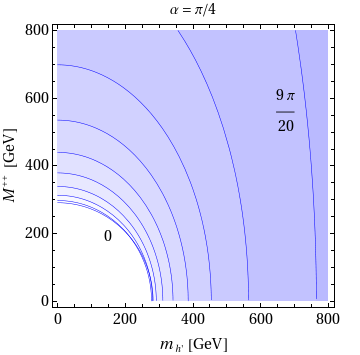
(b)

Figure 4: Allowed regions for the heavy neutral and doubly charged Higgs boson masses for various values of mixing angles in the doublet-septet model. The excluded regions are shaded. On the left figure $\beta$ is fixed at $\pi/4$ and $\alpha$ is increased from the left to right curves in steps of $\pi/20$. On the right figure, $\alpha$ is fixed at $\pi/4$ and $\beta$ increases from left to right in steps of $\pi/20$.

The case $\alpha=\beta=\pi/2$ again corresponds to having EW symmetry broken solely by the doublet Higgs. The doubly charged state from the septet therefore does not couple to the vector bosons, so that its mass is not constrained by unitarity. On the other hand, the mixing between the neutral states from both multiplets is maximal, so that $h$ is actually purely the neutral component of the septet. This does lead to a constraint $m_{h^{\prime}}\mbox{\raisebox{-2.58334pt}{~{}$\stackrel{{\scriptstyle<}}{{\sim}}$~{}}}900$ GeV but since the $126$ GeV Higgs does not couple to $W$ in this case, the situation is clearly unphysical. The opposite (and again unphysical) case of $\alpha=\pi/2,~{}\beta=0$, where the EW symmetry is broken purely by the septet VEV, leads to $M^{++}\lesssim 300$ GeV while leaving $m_{h^{\prime}}$ unconstrained. Two intermediate cases are shown in Fig. 4. The perturbative unitarity bounds on the extra Higgs masses for this case, as one can see, are quite stringent.

(a)

(b)

Figure 5: Conservative perturbative unitarity upper bounds on $m_{h^{\prime}}$ (5a, for $M^{++}=0$) and $M^{++}$ (5b, for $m_{h^{\prime}}=0$) as a function of mixing angles in the doublet-septet model. The bounds are periodic in $\alpha$ and we have centered the figures around the value of $\alpha$ where the bound is strongest.

Conservative bounds on the heavy Higgs masses, implied by perturbative unitarity in the doublet-septet model are shown in Fig. 5, assuming the lighter neutral Higgs mass $m_{h}=126$ GeV. In Fig. 5a (5b) the positive definite contribution of $M^{++}$ ($m_{h^{\prime}}$) in equation (19) has been ignored. In both figures the white regions correspond to small couplings $a_{h^{\prime}}$ and $b$, implying therefore very weak bounds on the Higgs masses.

Similar bounds on the masses of the two singly charged Higgses, $M_{1}^{+}$ and $M_{2}^{+}$, implied by perturbative unitarity in the $WZ$ channel are shown in Fig. 6. The value for the singly charged Higgs mixing angle $\gamma$ is taken to be $\pi/6$ for all cases. The bound is obtained for two different values of the heavy neutral Higgs mass, $m_{h^{\prime}}=136$, and 300 GeV respectively. In each case, one of the mixing angles $\alpha$ and $\beta$ is kept constant while the other is varied. Again, for the case that the septet takes appreciable part in the electroweak symmetry breaking ($\beta$ is not close to $\pi/2$), at least one of the charged Higgs bosons is bound to be relatively light.

(a)

(b)

(c)

(d)

Figure 6: Allowed regions for the singly charged Higgs boson masses for various values of mixing angles in the doublet-septet model. The heavy neutral Higgs masses have been taken to be 136 GeV (top row) and 300 GeV (bottom row). Shaded regions are excluded. On the left column $\beta$ is fixed at $\pi/4$ while $\alpha$ is increased from the left to right curves in steps of $\pi/20$. On the right column $\alpha$ is fixed at $\pi/4$ and $\beta$ increases from left to right in steps of $\pi/20$. For all of the above figures $\gamma$ has been fixed at $\pi/6$.

IV.3 The sum rule for $W^{+}_{L}W^{-}_{L}\to t\bar{t}$

A sum rule for $W^{+}_{L}W^{-}_{L}\to t\bar{t}$ is useful in constraining the couplings of the neutral scalars to the top-quark, which contribute to the amplitudes for production of these states in $gg$-fusion and for the decay into $\gamma\gamma$ and $\gamma Z$. The Feynman diagrams contributing to $W^{+}_{L}W^{-}_{L}\to t\bar{t}$ are shown in Fig. 7. The growth with one power of $s$ cancels among diagrams 7(a) and 7(b), resulting in a leading contribution that grows as $\sqrt{s}$.

We denote the coupling of the $i^{\text{th}}$ neutral, physical CP-even scalar to $\bar{t}t$ by $\lambda_{i}/\sqrt{2}$, so that $\lambda=gm_{t}/\sqrt{2}M_{W}$ in the SM as usual. Insisting that the growth with $\sqrt{s}$ is cancelled by the Higgs exchange diagram 7(c), we derive the sum rule

$$\frac{gm_{t}}{\sqrt{2}M_{W}}-\sum_{i}a_{i}\lambda_{i}=0,$$ (39)

where, as before, we denote by $a_{i}=(R^{T})_{ij}\tilde{a}_{j}$ and $\lambda_{i}=(R^{T})_{ij}\tilde{\lambda}_{j}$ the couplings of the physical, mass eigenstate Higgs to $W^{+}W^{-}$ and $\bar{t}t$, respectively, where $R$ is an orthogonal matrix, transforming weak eigenstates into the physical ones. The above equation has a simple interpretation. The sum of the couplings of the various scalars to the top quark has to be such that when the $i^{\text{th}}$ scalar is replaced by its expectation value, $v_{i}$, it gives the top quark mass term: $m_{t}=\sum\tilde{\lambda}_{i}v_{i}/\sqrt{2}$. One can see this by writing the above sum rule in the weak eigenbasis,

$$\frac{gm_{t}}{\sqrt{2}M_{W}}-\sum_{i}\tilde{a}_{i}\tilde{\lambda}_{i}=0.$$ (40)

Using $v_{i}=\tilde{a}_{i}(2M_{W}/g)$, one can see that this exactly reproduces the expression for the top quark mass. The sum rule is more conveniently written as per Eq. (2) in terms of the deviation of each Yukawa coupling from the SM value, $\lambda_{i}=(gm_{t}/\sqrt{2}M_{W})c_{ti}$, thus

$$\sum_{i}a_{i}c_{ti}=1.$$ (41)

(a)

Figure 7: $W^{+}W^{-}\to t\bar{t}$ scattering in the presence of a generic Higgs sector. $W^{3}$ in diagram b denotes the exchange of the $Z$ boson and the photon. Similarly, the $h$ in diagram c stands for a generic neutral Higgs boson.

Again, only the neutral Higgs from an $SU(2)$-doublet may couple to $\bar{t}t$. For example, if only the first Higgs is from a doublet, then $\lambda_{i}=(R^{T})_{i1}\tilde{\lambda}_{1}$, and $\sum\lambda_{i}^{2}=\tilde{\lambda}_{1}^{2}$, or $\sum c^{2}_{ti}=1/a_{1}^{2}\geq 1$.

The sum rule (39) has immediate phenomenological implications. It is saturated by any Higgs that has SM-like couplings to both $W^{+}W^{-}$ and $\bar{t}t$. It follows that either one or the other of these couplings for additional Higgses must vanish or there must be at least two additional Higgses with canceling contributions. That is, if a second Higgs-like resonance is discovered with near SM-like couplings, then a third one must also exist. Moreover, both of these resonances would have SM-like cross section for $gg\to h\to WW$, and one of them would have enhanced decay rate into $\gamma\gamma$ (since the $t$-loop and the $W$-loop contributions would interfere constructively).

Similar sum rules apply to the rest of quarks and all charged leptons. If the 126 GeV Higgs is observed not to decay (or have suppressed decays) to any one quark or charged lepton it follows immediately from the sum rule that there must be at least another CP-even neutral Higgs.

V Model Independent Analysis

V.1 Neutral Higgses

Figure 8: Region in the $a_{h^{\prime}}$-$c_{t}^{\prime}$ parameter space consistent with the unitarity constraint of Eq. (39) assuming $a_{h}$ and $c_{t}$ are determined from the 126 GeV Higgs data. The orange and brown regions are compatible with 126 GeV Higgs data at the 68% and 95% CL, respectively. For reference, the figure has been superimposed on the fit in Fig. 1 to the CMS data suggesting a Higgs resonance at 136 GeV.

In general, the couplings of any extra neutral Higgs, $h^{\prime}$, are related to the couplings of the $126$ GeV state $h$ via unitarity constraints of Section IV. In the following, we assume that there is only one additional neutral CP-even Higgs, and possibly some charged Higgs bosons. Here we focus on the sum rule involving the couplings to top quarks and vector-bosons, Eq. (41), since it doesn’t include the charged Higgs couplings and is therefore the most robust:

$$a_{h^{\prime}}c_{t}^{\prime}=1-a_{h}\,c_{t}.$$ (42)

Figure 9: Projection of the viable parameter space assuming all the errors are reduced by a factor of 2 (left plot) and 5 (right plot).

By fitting $a_{h}$ and $c_{t}$ to the existing 126 GeV Higgs data, we determine the allowed values for the quantity $a_{h}c_{t}$ at 68% and 95% CL. Using the sum rule (42), the allowed region can be mapped onto the $a_{h^{\prime}}$ – $c_{t}^{\prime}$ plane. The result is shown in Fig. 8, where regions in the $a_{h^{\prime}}$ – $c_{t}^{\prime}$ plane compatible with the 126 GeV Higgs data at the 68% and 95% CL are depicted in orange and brown, respectively. This is superimposed on Fig. 1 of the parameter estimation in light of the CMS 136 GeV higgs-like resonance data. One can see that only a small portion of $a_{h^{\prime}}$ – $c_{t}^{\prime}$ parameter space, allowed by current CMS measurements on the $136$ GeV resonance is actually consistent with the 126 GeV Higgs data. It is important to note that the bound from Eq. (42) is independent of the masses of the Higgs bosons. Thus, even if the excess at 136 GeV is not confirmed, the orange and brown regions in Fig. 8 will still be the favored regions for the couplings of a second Higgs boson in any model with exactly two neutral Higgses.

It is interesting to see how an increase in precision of the Higgs measurements would affect the allowed $a_{h^{\prime}}$ – $c_{t}^{\prime}$ parameter space. For this, we show in Fig. 9 projections assuming that all central values of measurements remain intact, while the errors are reduced by a factor of 2 and 5. One can see that under such assumptions, the increased accuracy in the measurements would render the CMS data on the 136 GeV resonance incompatible with the data on the 126 GeV Higgs.

V.2 Doubly Charged Higgses

The primary decay modes for a doubly charged Higgs are to a pair of same-sign $W$ bosons and to a pair of singly charged same sign Higgs bosons. In the analysis below we assume $\text{Br}(h^{++}\to W^{+}W^{+})=100\%$, since $\Gamma(h^{++}\to h^{+}h^{+})$ is model dependent, determined by parameters in the Higgs potential. Searches for new physics with same-sign dileptons are sensitive to $h^{++}\to W^{+}W^{+}$, and can be used to constrain the parameter space of the doubly charged Higgs. As above, the model independent interaction is defined as follows,

$$\mathcal{L}_{int}=gM_{W}bW_{\mu}^{-}W^{\mu-}h^{++}+\text{h.c.}.$$ (43)

Single $h^{\pm\pm}$ production at the LHC occurs through $W$ boson fusion and in association with a $W$ boson, both of which can lead of a signature of same-sign dileptons and jets. Results of a search for this signature using the full LHC Run 1 dataset are given in Ref. Chatrchyan:2013fea , which expands on searches using less data Chatrchyan:2012sa ; Chatrchyan:2012paa . Information about event selection efficiencies is provided in Chatrchyan:2013fea ; Chatrchyan:2012sa ; Chatrchyan:2012paa such that models of NP may be constrained in an approximate way using generator-level MC studies, i.e., without performing a full detector simulation. This prescription is known to reproduce the results of the full CMS analysis to within 30% Chatrchyan:2012sa .

FeynRules Christensen:2008py was used to implement Eq. (43) in MadGraph 5 Alwall:2011uj with MSTW2008 LO PDFs Martin:2009iq , which was used to generate events for the analysis. The kinematic requirements placed on charged leptons were $p_{T}>20$ GeV (high-$p_{T}$ analysis) and $|\eta|<2.4$, and on jets were $p_{T}>40$ GeV and $|\eta|<2.4$. The so-called SR5 in the high-$p_{T}$ analysis was the single most constraining signal region. This signal region is defined by having 2-3 jets with 0 $b$-tags, $E_{T}^{\text{miss}}>120$ GeV, and $H_{T}\in[200,400]$ GeV. 12 events were observed in SR5 compared to an expected background of $20\pm 7$. Using confidence interval calculator program of Ref. Barlow:2002bk , we place an upper limit of 6.1 non-background events at 95% CL assuming a signal efficiency uncertainty of 13%. The upper limit is very weakly dependent on this uncertainty such that it is still 6.1 when the signal efficiency uncertainty is taken to be 20%.

The results of this analysis are shown in Fig. 10. The blue curve is the upper limit of 6.1 events with the pink band corresponding to the 30% uncertainty in the analysis method. The parameter space above and to the left of the blue curve is ruled out by the CMS search. The green line is the perturbative unitarity bound, Eq. (19), neglecting the 126 GeV Higgs. The parameter space above and to the right of the green curve is ruled out by perturbative unitarity.

Figure 10: Viable parameter space for a doubly charged Higgs based on a search for NP in events with same-sign dileptons and jets. The blue curve is the upper limit with its uncertainty given by the pink band. The green line is the perturbative unitarity bound. The parameter space shown in gray is ruled out.

The enhancement of the exclusion near $m_{h^{++}}\approx 2m_{W}$ is due to both $W$’s in the decay chain going on-shell. Note that we did not simulate signal-background interference, which is relevant when the NP cross section approaches the SM cross section. This occurs in the pink band. We don’t claim this region is ruled out as it represents the uncertainty in the upper limit of the exclusion. We also did not perform a comprehensive study of the effect of more than one new Higgs particle as this would have required introducing several additional parameters. However, we did investigate a few benchmark points in the double-septet model with the result that the exclusion does not change significantly if the mass of the second Higgs is at least a few hundred GeV, which is expected as the Higgs cross section drops steadily with an increase in mass.

VI Specific Models

Consider next various explicit realizations of electroweak symmetry breaking. For specific, perturbative models the sum rules derived by requiring that longitudinally polarized gauge boson scattering grows no faster than logarithmically with center of mass energy are automatically satisfied. But sum rules limiting the masses of various Higgs bosons are genuinely new inputs. For each of the models we study we fit both to the 126 GeV Higgs data and to the 126 GeV and 136 GeV Higgs data combined. Tab. 1 shows the minimum $\chi^{2}$ values as well as the number of degrees of freedom, $N$, in each of the models we study in this section. The table also shows, for comparison, the results of the model independent fits of the previous section, in which $a_{h}$, $c_{t}$, $c_{b}$ and $c_{\tau}$ are treated as independent parameters in the fit to 126 GeV Higgs data while the set of independent parameters is enlarged to include $a_{h^{\prime}}$, $c_{t}^{\prime}$, $c_{b}^{\prime}$ and $c_{\tau}^{\prime}$ for the fit to the combined 126 and 136 GeV data. Here $c_{f}$ ($c_{f}^{\prime}$) refers to the modification of neutral Higgs boson, $h$ ($h^{\prime}$), coupling to $\bar{f}f$ with respect to SM Higgs boson coupling.

Models	&3126 GeV Fit36		126 & 136 GeV Fit
	a $\chi^{2}/N$a	$N$	a $\chi^{2}/N$a	$N$
Model independent	0.29	14	0.32	12
Douplet-septet	0.31	16	0.71	18
Georgi-Machacek	0.31	16	0.60	18
2HDM-II	0.31	16	0.56	18
2HDM-III	0.28	14	0.60	16

Table 1: Minimum $\chi^{2}$ values for various models studied. Here $N$ stands for the number of degrees of freedom.

VI.1 The Doublet-Septet Model

The doublet-septet model contains two Higgs fields: the standard (weak) isospin-1/2 and an isospin-3 (septet) multiplets. We have introduced earlier various aspects of this model in several different sections, so it is convenient to collect, review and expand on them here. As noted above, the septet contains a doubly charged Higgs, whose interactions with the vector bosons can be written as in IV.2.2,

$$\mathcal{L}_{int}\supset\sqrt{15}\frac{M_{W}^{2}}{v_{\text{EW}}}\cos\beta\left(W^{-}_{\mu}W^{-\mu}h^{++}+W^{+}_{\mu}W^{+\mu}(h^{++})^{\star}\right)~{},$$ (44)

where the mixing angle, $\beta$, is defined as $\tan\beta=v_{1}/(4v_{2})$. Here $v_{1}$ ($v_{2}$) denotes the VEV of the doublet (septet). Note that $M_{W}^{2}\cos\beta/v_{\text{EW}}=g^{2}v_{2}$, or $4v_{2}=v_{\text{EW}}\cos\beta$ and $v_{1}=v_{\text{EW}}\sin\beta$. The interactions of the neutral Higgses are given by

$$\mathcal{L}_{int}\supset\frac{2}{v_{\text{EW}}}\left(M_{W}^{2}W^{+}_{\mu}W^{-\mu}+\frac{1}{2}M_{Z}^{2}Z_{\mu}Z^{\mu}\right)\left((s_{\beta}c_{\alpha}-4c_{\beta}s_{\alpha})h+(s_{\beta}s_{\alpha}+4c_{\beta}c_{\alpha})h^{\prime}\right),$$ (45)

where $h,h^{\prime}$ are the neutral Higgs states in the mass basis, related to those in the weak basis, $h^{0}_{2}$ and $h^{0}_{7}$, by

$$\begin{pmatrix}h^{0}_{2}\\ h^{0}_{7}\end{pmatrix}=\begin{pmatrix}c_{\alpha}&s_{\alpha}\\ -s_{\alpha}&c_{\alpha}\end{pmatrix}\begin{pmatrix}h\\ h^{\prime}\end{pmatrix},$$ (46)

with $s_{\alpha}$, $c_{\alpha}$ standing for the sine and cosine of $\alpha$, the mixing angle between the weak mass bases. We identify $h$ with the 126 GeV resonance, recently discovered at the LHC Aad:2012tfa ; Chatrchyan:2012ufa . The couplings of the neutral Higgses to fermions are given by

$$\mathcal{L}\supset\left(\frac{\cos\alpha}{\sin\beta}h+\frac{\sin\alpha}{\sin\beta}h^{\prime}\right)\sum_{i}\frac{m_{f,i}}{v_{\text{EW}}}\bar{f}_{i}f_{i},$$ (47)

where $m_{f,i}$ denotes the mass of the $i^{\text{th}}$ fermion. The doubly charged Higgs obviously cannot couple to fermions at the renormalizable level. The above couplings give the parameters $a_{i}$ and $b$ displayed in (38), while the couplings to fermions are parametrized by

$$c_{f}=\cos\alpha/\sin\beta,\quad c_{f}^{\prime}=\sin\alpha/\sin\beta.$$

Figure 11: Allowed region of $a_{h^{\prime}}$-$c_{t}^{\prime}$ for the doublet-septet model from a fit to the 126 GeV Higgs data. The best fit value is indicated by a blue star, and the orange and brown regions give the 68% and 95% CL regions, respectively. The underlying green/yellow regions are from the model independent fit to the 136 GeV data in Fig. 1.

One can infer the bounds on the extra neutral resonance from the available data on the 126 GeV Higgs in much the same way as for the case of the model-independent fit outlined above. The fit to the 126 GeV data, combined with the condition of perturbative unitarity in the $WW\to t\bar{t}$ channel significantly reduces the allowed parameter space for the $136$ GeV Higgs couplings. The 68% and 95% CL regions in the $a_{h^{\prime}}-c_{t}^{\prime}$ plane (defined in the same way as for the model-independent fit) allowed by the 126 GeV data are shown in orange and brown in Fig. 11. The best fit value is marked by a star; the corresponding (minimum) has $\chi^{2}_{DS}=4.96$ for 16 degrees of freedom. The figure shows limited overlap between the model independent fit to the 136 GeV data (in green/yellow) and the model specific fit to the 126 GeV data (in orange/brown). Alternatively, a global fit to both 126 and 136 GeV data gives a higher minimum, with $\chi^{2}_{DS}$ at 12.71 for 18 degrees of freedom.

Another bound on a second Higgs can be obtained from the ATLAS and CMS searches for SM-like Higgs bosons in the $WW$ and $ZZ$ channels ATLAS-CONF-2013-013 ; ATLAS-CONF-2013-067 ; CMS-PAS-HIG-12-024 ; CMS-PAS-HIG-13-002 ; CMS-PAS-HIG-13-003 ; CMS-PAS-HIG-13-008 ; CMS-PAS-HIG-13-014 . Taken at face value, our combination of these bounds in Appendix B rules out Higgs bosons that couple to $WW$ and $ZZ$ with SM strength at 95% CL for $m_{h^{\prime}}=128-1000$ GeV. However, there is no reason to expect neutral Higgs particles should couple to EW gauge bosons with SM strength in multi-Higgs models. The couplings must satisfy the model-dependent and model-independent sum rules, Eqs. (10) and (17), respectively, but both of these allow for a range of coupling strengths. Instead, for a given set of parameters in a model, one must compare the predicted signal strength against the curve in Fig. 16 to determine the range(s) for which $m_{h^{\prime}}$ is ruled out. The signal strength of $h^{\prime}$ in the $WW+ZZ$ channel is given by

$$\mu(h^{\prime}\to WW+ZZ)=\frac{c_{f}^{\prime 2}\sigma_{ggF+t\bar{t}h^{\prime}}+a_{h^{\prime}}^{2}\sigma_{VBF+Vh^{\prime}}}{\sigma_{ggF+t\bar{t}h^{\prime}}+\sigma_{VBF+Vh^{\prime}}}\frac{a_{h^{\prime}}^{2}}{c_{f}^{\prime 2}Br_{f\bar{f}}+a_{h^{\prime}}^{2}Br_{VV}+c_{f}^{\prime 2}Br_{gg}},$$ (48)

where $\sigma$ ($Br$) is the expected SM cross-section (branching ratio) for the Higgs boson with mass $m_{h^{\prime}}$, with $f=\tau,c,b,t$, $V=W,Z$. All cross sections and branching ratios in (48) are taken from Ref. Dittmaier:2011ti . Here we implicitly assume $h^{\prime}$ has the same decay channels available as $h$, but if heavy enough new channels may become available, e.g., it could decay to a pair of scalars and/or a pseudoscalar and a neutral vector boson ($AZ$), and these channels may have significant branching fractions. See Ref. Grinstein:2013npa for an analysis of these decay modes in the Type-II two Higgs doublet model.

For given values of $a_{h^{\prime}}$ and $c^{\prime}_{f}$ (or $\alpha$ and $\beta$), $\mu(h^{\prime}\to WW+ZZ)$ as a function of $m_{h^{\prime}}$ can be compared against the data in Fig. 16. The parameter space that is ruled out by searches for additional Higgs bosons is given by the blue regions in Fig. 12 for 6 different values of $m_{h^{\prime}}$. In addition, we show in red the complement of the 95% CL region of parameter space from the fit to the 126 GeV Higgs data (the complement to the orange and brown region in Fig. 11). Finally, the orange region is ruled out by perturbative unitarity. It is essentially the bound from Fig. 5a plotted as a function of $a_{h^{\prime}}$ and $c^{\prime}_{f}$ rather than $\alpha$ and $\beta$. The bounds in Fig. 2 have consequences for the interpretation of the excess at 136 GeV in CMS-PAS-HIG-13-016 as a second neutral Higgs boson. In the upper-left panel of Fig. 12 we also plotted the allowed region for $a_{h^{\prime}}$ and $c^{\prime}_{f}$ from Fig. 2b. We see that for the 136 GeV Higgs in the doublet-septet model there is very limited overlap between the 95% CL-allowed region from the exclusion limits from searches for heavy Higgs bosons in the $WW$ and $ZZ$ channels and the 95% CL-allowed region from data on the 126 GeV Higgs.

(a)

(b)

(c)

(d)

(e)

(f)

Figure 12: Parameter space in the doublet-septet model that is ruled out at the 95% CL due to searches for heavy Higgses (blue), 126 GeV Higgs data (red) and perturbative unitarity (orange) for various values of $m_{h^{\prime}}$. For the $m_{h^{\prime}}=136~{}\text{GeV}$ case, the figure is superimposed on Fig. 2 that shows the 68% and 95% CL model-independent regions compatible with the excess seen by CMS, displaying little overlap with the allowed (white) region from this analysis.

VI.2 Other Models

In this subsection we compare the result from the model independent fit to explicit models with extended Higgs sectors. In all the models we consider electroweak symmetry breaking is perturbative.

VI.2.1 Georgi-Machacek Model

Figure 13: Region of the $a_{h^{\prime}}$-$c_{t}^{\prime}$ parameter space consistent with the fit to the GM model. The orange and brown regions are compatible at 68% and 95% CL, respectively and the best fit value is indicated by a blue star. The underlying green/yellow regions are from the model independent fit to the 136 GeV data in Fig. 1. The darker blotches contained within the green region are overlaps of brown and green.

The Georgi-Machacek(GM) model consists of one electroweak doublet of hypercharge 1/2 and two electroweak triplets with hypercharge 0 and 1. For a recent phenomenological study of the model see Ref. Chiang:2012cn and references therein. The electroweak VEV is given by $v_{\text{EW}}^{2}=v_{\phi}^{2}+8v_{\Delta}^{2}$ with $\tan\beta=v_{\phi}/2\sqrt{2}v_{\Delta}$, where $v_{\phi}$ and $v_{\Delta}$ are the VEVs of the doublet and the two triplets respectively. There are three CP even neutral scalar fields in the GM model, $\phi_{r}$, $\tilde{H}_{1}^{0}$ and $H_{5}^{0}$. These fields are related to the physical states by

$$\begin{pmatrix}\phi_{r}\\ \tilde{H}_{1}^{0}\\ H_{5}^{0}\end{pmatrix}=\begin{pmatrix}c_{\alpha}&s_{\alpha}&0\\ -s_{\alpha}&c_{\alpha}&0\\ 0&0&1\end{pmatrix}\begin{pmatrix}h\\ h^{\prime}\\ H_{5}^{0}\end{pmatrix},$$ (49)

where $c_{\alpha}=\cos\alpha$ and $s_{\alpha}=\sin\alpha$. The couplings to the vector boson and fermion pairs for the two Higgses are given as follows

$$a_{h}=\frac{1}{3}\left(3c_{\alpha}s_{\beta}-2\sqrt{6}s_{\alpha}c_{\beta}\right),~{}c_{f}=\frac{c_{\alpha}}{s_{\beta}},~{}a_{h^{\prime}}=\frac{1}{3}\left(3s_{\alpha}s_{\beta}+2\sqrt{6}c_{\alpha}c_{\beta}\right),~{}c^{\prime}_{f}=\frac{s_{\alpha}}{s_{\beta}}~{}.$$

By performing a fit to the 126 GeV data, we obtain a minimum $\chi^{2}_{GM}=4.96$ for 16 degrees of freedom. Within the context of the GM model, the couplings $c_{h^{\prime}}$ and $c_{t}^{\prime}$ consistent with the model-independent fit are shown in Fig. 13 where again the best fit value is marked by a star. Alternatively, a global fit to both 126 and 136 GeV data gives a higher minimum $\chi^{2}_{GM}$ at 10.84 for 18 degrees of freedom.

VI.2.2 Two-Higgs-Doublet Model

Figure 14: Region of the $a_{h^{\prime}}$-$c_{t}^{\prime}$ parameter space consistent with the fit to the Type-II (left) and Type-III (right) 2HDM. The orange and brown regions are compatible at 68% and 95% CL, respectively. The best fit value for the Type-III model is indicated by a blue star, while it is at ($a_{h^{\prime}},\,c_{t}^{\prime}$) = (-0.02,-3.14) for the Type-II 2HDM. The underlying green/yellow regions are from the model independent fit to the 136 GeV data in Fig. 1.

There are many variations of the two-Higgs-doublet models, see Ref Branco:2011iw for a recent review. Here we will focus on two explicit realizations, the so called type-II (2HDM-II) and type-III (2HDM-III). In 2HDM-II a discrete $Z_{2}$ symmetry is imposed to forbid tree-level flavor changing neutral currents (FCNC). In this case the neutral scalar couplings to vectors and fermions are determined by two angles, $\alpha$ and $\beta$. The angle $\alpha$ is the mixing angle for the two CP-even neutral scalars, while $\tan\beta$ is given by the ratio of the two VEVs. The coupling modifiers for the two Higgses are given in this case by the following expressions

$$a_{h}=\sin(\alpha+\beta),~{}c_{t}=c_{c}=\frac{c_{\alpha}}{s_{\beta}},~{}c_{b}=c_{\tau}=\frac{s_{\alpha}}{c_{\beta}},~{}a_{h^{\prime}}=\cos(\alpha+\beta),~{}c^{\prime}_{t}=c^{\prime}_{c}=\frac{s_{\alpha}}{s_{\beta}},~{}c^{\prime}_{b}=c^{\prime}_{\tau}=\frac{c_{\alpha}}{c_{\beta}}.$$

By performing a fit to the 126 GeV data, we obtain a minimum $\chi^{2}_{2HDM-II}=4.91$ for 16 degrees of freedom. Within the context of the 2HDM-II, the couplings $a_{h^{\prime}}$ and $c_{t}^{\prime}$ consistent with the model-independent fit are shown in Fig. 14. Alternatively, a global fit to both 126 and 136 GeV data gives a higher minimum $\chi^{2}_{2HDM-II}$ at 10.13 for 18 degrees of freedom.

In 2HDM-III where the discrete $Z_{2}$ symmetry is not imposed, there in general are flavor changing neutral currents. However, we will ignore FCNC and proceed to study the neutral scalar couplings to vectors and fermions in this model. Unlike in the 2HDM-II, here the couplings to the third generation fermions, relevant for Higgs phenomenology, are characterized by three additional parameters $c_{t}$, $c_{b}$ and $c_{\tau}$ (the couplings to the vector bosons are the same as in 2HDM-II). Fitting to the 126 GeV data, we obtain a minimum $\chi^{2}_{2HDM-III}=3.93$ for 14 degrees of freedom, while fitting to both 126 and 136 GeV data gives a higher minimum $\chi^{2}_{2HDM-III}$ at 9.61 for 18 degrees of freedom.

VII Consistency with dispersion relations

Dispersion relations have been used to constrain models with zero Distler:2006if and one Low:2009di ; Falkowski:2012vh ; Urbano:2013aoa Higgs particles. It is straightforward to generalize those to the case of multi-Higgs models. For self-completeness, we give a detailed derivation of the dispersion relations of Refs. Low:2009di ; Falkowski:2012vh ; Urbano:2013aoa and their multi-Higgs generalizations in appendix C.

One such dispersion relation, that is of particular interest to us, is written as follows

$$\frac{d{\mathcal{A}}}{ds}\bigg{|}_{s=0}=\frac{2w^{0}+w^{1}-w^{2}}{\pi}\int_{0}^{\infty}\frac{ds}{s}\left[\sigma_{+-}-\sigma_{++}\right],$$ (50)

where $\sigma_{+-}$ denotes the total cross section for a longitudinally polarized $W^{+}W^{-}$ scattering, and likewise for $\sigma_{++}$. Alternatively, using the equivalence theorem one may calculate $\sigma_{+-}$ and $\sigma_{++}$ as the cross section for $\pi^{+}\pi^{-}\to\textit{anything}$ and $\pi^{+}\pi^{+}\to\textit{anything}$, in a nonlinear sigma model for electroweak symmetry breaking. Below we refer to this as “pion scattering,” keeping in mind that we are really describing longitudinally polarized vector boson scattering. The amplitude ${\mathcal{A}}$ is expanded in terms of amplitudes of definite isospin (isospin-$0,1,2$ respectively), ${\mathcal{A}}=\sum_{I}w^{I}T^{I}$, with coefficients $w^{I}$. The integral in the once subtracted dispersion relation (50) is not generally convergent. Barring a cancellation in the difference of cross sections, a cross section saturating the Froissart bound would give a divergent integral. Therefore, in order to be able to use (50) e.g. for strongly coupled theories, one has to assume that the UV cross-sections exhibit milder high-energy behavior than allowed by the Froissart bound.

On the other hand, for perturbative models with definite UV field content like the ones considered above, the cross sections do give convergent integrals. However, in those cases both sides of the dispersion relation can be calculated perturbatively to check that it is identically satisfied, once unitarity constraints are imposed.

One can readily study the implications of the dispersion relation (50) and their consistency with the relations obtained from perturbative unitarity above. Let us for definiteness concentrate on $\pi^{+}\pi^{-}$ scattering. Using eqs. (81) and (68) of appendix C, the decomposition of the corresponding amplitude into the isospin eigenbasis can be written as follows, ${\mathcal{A}}_{\pi^{+}\pi^{-}}=\sum_{I}w^{I}T^{I}$, with $w^{0,1,2}=(1/3,~{}1/2,~{}1/6)$, so that $2w^{0}+w^{1}-w^{2}=1$. The once subtracted dispersion relation for charged pion scattering thus implies

$$\frac{d{\mathcal{A}}_{\pi^{+}\pi^{-}}}{ds}\bigg{|}_{s=0}=\frac{1}{\pi}\int_{0}^{\infty}\frac{ds}{s}\left[\sigma_{+-}-\sigma_{++}\right]~{}.$$ (51)

Assuming, as required by unitarity at order $\hbar^{0}$, that all contributions to the amplitude that grow with $s$ cancel, one readily obtains the following tree-level expression for the finite piece of the forward scattering amplitude

$${\mathcal{A}}_{\pi^{+}\pi^{-}}=\frac{s}{v^{2}}\left(\sum_{i}\frac{a_{i}^{2}m_{h_{i}}^{2}}{m_{h_{i}}^{2}-s}-\sum_{r}\frac{4b_{r}^{2}M_{r}^{++2}}{M_{r}^{++2}+s}\right)~{}.$$ (52)

Here the sums are performed over various neutral and doubly charged Higgs bosons. Straightforward differentiation then yields

$$\frac{d{\mathcal{A}}_{\pi^{+}\pi^{-}}}{ds}\bigg{|}_{s=0}=\frac{\sum_{i}a^{2}_{i}-4\sum_{r}b_{r}^{2}}{v^{2}}~{}.$$ (53)

Figure 15: Diagrams contributing to (a) $\sigma_{+-}$ and (b) $\sigma_{++}$ in (51).

Furthermore, at order $1/v^{2}$, there is a single diagram contributing to each of the terms on the right hand side of (52); the tree-level annihilation $\pi^{+}\pi^{-}\to h_{i}$ contributes to $\sigma_{+-}$, while $\sigma_{++}$ receives its only contribution from $\pi^{+}\pi^{+}\to\phi_{r}^{++}$. These cross sections are given as follows

$$\sigma_{+-}=\sum_{i}\frac{\pi a_{i}^{2}s}{2v^{2}m^{2}_{h_{i}}}\delta\left(\sqrt{s}-m_{h_{i}}\right),\quad\sigma_{++}=\sum_{r}\frac{4\pi b_{r}^{2}s}{2v^{2}M_{r}^{++2}}\delta\left(\sqrt{s}-M^{++}\right)~{},$$ (54)

where the delta functions remain after integration over the single particle phase space. Using these expressions, it is straightforward to show that

$$\frac{1}{\pi}\int_{0}^{\infty}\frac{ds}{s}\left[\sigma_{+-}-\sigma_{++}\right]=\frac{\sum_{i}a^{2}_{i}-4\sum_{r}b_{r}^{2}}{v^{2}}=\frac{d{\mathcal{A}}_{\pi^{+}\pi^{-}}}{ds}\bigg{|}_{s=0}~{}.$$ (55)

As advertised, the dispersion relation is identically satisfied for theories that respect unitarity at order $\hbar^{0}$. The only input that we used from unitarity in the above analysis is that the amplitudes do not grow at large center of mass energy, so that the integral of the cross sections in the once subtracted dispersion relation is convergent and well-defined. In fact, at the (tree) level we are interested in here, the singularity structure on the complex $s$ plane is drastically simplified. Indeed, in the limit $\hbar\to 0$ there are no cuts on the real axis, only singularities corresponding to on-shell poles from heavy particle exchange contribute. The imaginary part of amplitudes corresponding to exchange of a particle of mass $M$ is proportional to

$$\text{Im}\frac{1}{p^{2}-M^{2}+i\epsilon}=-\pi\delta(p^{2}-M^{2})~{},$$ (56)

and only has support on the heavy particle pole. This is also evident from (54), given that the cross section is related to the imaginary part of the forward scattering amplitude through the optical theorem. The discontinuity of the amplitude across these poles gives the only contribution to the right hand side of (51) at tree level. It is straightforward to extend this analysis beyond tree level, but the main result, that the dispersion relation is identically satisfied for unitary theories that are weakly coupled over the full range of energy scales, is unchanged. Moreover, the dispersion relations do not imply the perturbative unitarity bounds on Higgs masses obtained in Sec. IV.

VIII Discussions and Conclusions

Charged scalars play a crucial role in unitarizing the vector-vector scattering amplitudes in a model with a weakly coupled Higgs sector. In the case of $W^{+}_{L}W^{-}_{L}\to W^{+}_{L}W^{-}_{L}$ scattering, the full amplitude does not grow with $s$ due to a cancellation between $s$- and $t$- channel contributions from neutral Higgses and $u$- channel contributions from doubly-charged Higgses. Similarly, the combined contribution of neutral and singly-charged Higgs bosons ensure that the amplitude for $Z_{L}Z_{L}\to W^{+}_{L}W^{-}_{L}$ does not grow with $s$. Not surprisingly, this cancellation holds for an arbitrary number of Higgs multiplets with arbitrary representations under $SU(2)_{L}\times U(1)_{Y}$.

Unitarity also places constraints on the spectrum of the Higgses and their couplings to fermions. The constraint on the spectrum depends strongly on the number and the representation of the multiplets involved in electroweak symmetry breaking. We studied this constraint in the doublet-septet model in section IV.2.3. The constraint on the couplings of neutral Higgses to fermions arises from unitarity requirement in $W^{+}_{L}W^{-}_{L}\to f\bar{f}$ channel. Unlike the bound on the spectrum, where detailed knowledge of Higgs multiplets is needed, the constraint on the couplings to fermions only depend on the knowledge of the number of neutral Higgses present in the model and not on the masses of the Higgs bosons.

Now we turn to discuss the interpretation of the 136 GeV excess observed in CMS diphoton signal as a second neutral Higgs. Since this excess has been only observed in the diphoton channel, we focus on studying the coupling of the putative second neutral Higgs to vector boson and top-quark (characterized by $a_{h^{\prime}}$ and $c^{\prime}_{t}$ respectively). We can be predictive on the couplings $a_{h^{\prime}}$ and $c^{\prime}_{t}$ if we assume that there are only two CP-even neutral Higgses in the spectrum. In this case unitarity in $W^{+}_{L}W^{-}_{L}\to t\bar{t}$ channel requires $a_{h^{\prime}}c^{\prime}_{t}=1-a_{h}c_{t}$. By deducing the coupling $a_{h}$ and $c_{t}$ from the 126 GeV Higgs data, we obtained the model-independent prediction of the coupling $a_{h^{\prime}}$ and $c^{\prime}_{t}$ shown in figure 8. We found there that the interpretation of the 136 GeV excess is in some tension with the 126 GeV Higgs data. Our projection of the situation assuming improved experimental precision in both the 126 and 136 GeV data show that if the 136 GeV excess persists, it cannot be explained by a second neutral Higgs in a model with only two neutral CP-even Higgses.

We can in fact improve on the prediction of the couplings of the second Higgs in Fig. 8 by further specifying the origin of the second Higgs particle. Figs. 11, 13 and 14 show the resulting fit in sample specific models, showing in all cases a reduction in the allowed region of parameter space. However, the allowed regions are qualitatively different for the various models we investigated, with obvious implications for the production mechanism in collider experiments. The most striking of these is for the 2HDM Type-II model, Fig. 14 (left pannel) , for which vector boson fusion is largely inoperative while the rate for gluon fusion could differ vastly from that of a SM Higgs.

Appendix A Physical Higgses Couplings

In this appendix we collect the couplings of the physical Higges. We denote the physical CP-even neutral Higgses by $h_{i}$, the singly charged Higgses by $\phi^{+}_{j}$ and the doubly charged by $\phi^{++}_{r}$. The couplings can be parametrized by

$$\begin{split}\mathcal{L}_{phys}&\supset gM_{W}W^{+\mu}W^{-}_{\mu}\sum_{i}a_{i}h_{i}+\frac{gM_{W}}{2}Z^{\mu}Z_{\nu}\sum_{i}d_{i}h_{i}-\frac{m_{f}}{v_{\text{EW}}}\sum_{i}c_{i}\bar{f}fh_{i}\\ &\quad+gM_{W}\left(Z^{\mu}W^{+}_{\mu}\sum_{j}f^{\phantom{+}}_{j}\phi^{+}_{j}+\text{h.c.}\right)+gM_{W}\left(W^{+\mu}W^{+}_{\mu}\sum_{r}b^{\phantom{+}}_{r}\phi^{++}_{r}+\text{h.c.}\right).\\ \end{split}$$ (57)

The value of the couplings $a$, $b$, …, $f$ depends on the detail of the Higgs sector— the number of electroweak multiplets and the size of each multiplet.

Here we recall the couplings of the Higgses in a generic representation of the electroweak gauge group from Sec. IV. This result can be easily extended to a case with an arbitrary number of electroweak multiplets. For definiteness, we take the Higgs field, $\Phi$, to transform in a $(2n+1)$-dimensional representation of $SU(2)_{L}$ with hypercharge $-m$, $-n\leq m\leq n$. To preserve electric charge the VEV of the multiplet must be in the $T^{3}=m$ component, $\langle\phi_{m}\rangle=v/\sqrt{2}$. Thus $\phi_{m\pm 2}$ corresponds to the doubly charged component and $\phi_{m\pm 1}$ is the singly charged component. Their interactions are

$$\begin{split}\mathcal{L}&\supset\frac{g^{2}v}{\sqrt{2}}\eta^{\mu\nu}\left[A\left(W^{+}_{\mu}W^{+}_{\nu}\phi_{m-2}+W^{-}_{\mu}W^{-}_{\nu}\phi_{m-2}^{*}\right)+B\left(W^{+}_{\mu}W^{+}_{\nu}\phi_{m+2}^{*}+W^{-}_{\mu}W^{-}_{\nu}\phi_{m+2}\right)\right]\\ &+\frac{1}{2}\eta^{\mu\nu}\left[g^{2}W^{+}_{\mu}W^{-}_{\nu}\left(n(n+1)-m^{2}\right)+(g^{2}+g^{\prime 2})Z_{\mu}Z_{\nu}m^{2}\right](v+\phi_{m})^{2}\\ &\qquad+\frac{v\cos\theta_{W}}{\sqrt{2}}~{}\bigg{[}Z^{\mu}W^{+}_{\mu}\left(D\phi_{m-1}+E\phi^{*}_{m+1}\right)+h.c.\bigg{]},\end{split}$$ (58)

where $g$ $(g^{\prime})$ is the $SU(2)$ ($U(1)$) couplings and

$$A =\frac{1}{2}\sqrt{\left[n(n+1)-(m-2)(m-1)\right]\left[n(n+1)-m(m-1)\right]},$$ (59)

$$B =\frac{1}{2}\sqrt{\left[n(n+1)-m(m+1)\right]\left[n(n+1)-(m+1)(m+2)\right]},$$

$$D =F\big{[}2(g^{2}+g^{\prime 2})m-g^{2}\big{]},$$

$$E =G\big{[}2(g^{2}+g^{\prime 2})m+g^{2}\big{]},$$

$$F =\sqrt{\tfrac{1}{2}\big{(}n(n+1)-m(m-1)\big{)}},$$

$$G =\sqrt{\tfrac{1}{2}\big{(}n(n+1)-m(m+1)\big{)}}.$$

We can relate the above parameters to the couplings of the physical Higgses, as in Eq. (57). The couplings of the physical Higgses are given by

$$gM_{W}a =g^{2}v\left[n(n+1)-m^{2}\right],$$ (60)

$$gM_{W}b_{1(2)} =\frac{g^{2}v}{\sqrt{2}}A\,(B),$$

$$gM_{W}d =2(g^{2}+g^{\prime 2})v\,m^{2},$$

$$(gM_{W}f)^{2} =\left(\frac{v\cos\theta_{W}}{\sqrt{2}}\,\frac{4m\,F\,G(g^{2}+g^{\prime 2})}{\sqrt{F^{2}+G^{2}}}\right)^{2}.$$

Note that one linear combination of $\phi_{m+1}$ and $\phi_{m-1}$ is eaten by the $W$.

Appendix B Higgs Data

Channel	($\mu_{V},\,\mu_{F}$)	($\Delta\mu_{V},\,\Delta\mu_{F}$)	$\rho$	Reference
ATLAS $\gamma\gamma$	(1.75, 1.62)	(1.25, 0.63)	-0.17	ATLAS-CONF-2013-012
CMS $\gamma\gamma$	(1.48, 0.52)	(1.33, 0.60)	-0.48	CMS-PAS-HIG-13-001
ATLAS ZZ	(1.2, 1.8)	(3.9, 1.0)	-0.3	ATLAS-CONF-2013-013
CMS ZZ	(1.7, 0.8)	(3.3, 0.6)	-0.7	Chatrchyan:2013mxa
ATLAS WW	(1.57, 0.79)	(1.19, 0.55)	-0.18	ATLAS-CONF-2013-034
CMS WW	(0.71, 0.72)	(0.96, 0.32)	-0.23	CMS-PAS-HIG-13-005
ATLAS $\tau\bar{\tau}$	(1.50, 1.04)	(1.05, 1.83)	-0.50	ATLAS-CONF-2013-108
CMS $\tau\bar{\tau}$	(1.55, 0.66)	(1.26, 1.21)	-0.45	CMS-PAS-HIG-13-005
Combined $Vh,\,h\to b\bar{b}$	(0.9, -)	(0.3, -)	-	ATLAS-CONF-2013-079 ; CMS-PAS-HIG-13-012 ; TEVNPH:2012ab
Combined $t\bar{t}h,\,h\to b\bar{b}$	(-, -0.1)	(-,1.8)	-	ATLAS-CONF-2012-135 ; CMS-PAS-HIG-13-019

Table 2: The signal strengths with their uncertainties and correlations for the 126 GeV resonance used in the fit.

Collaboration	Channel	$\sqrt{s}\,[\text{TeV}]$	$\mathcal{L}\,[\text{fb}^{-1}]$	Range $m_{h^{\prime}}$ probed [GeV]
ATLAS ATLAS-CONF-2013-013	$h^{\prime}\to ZZ\to 4\ell$	$8$	$20.7$	$110-1000$
ATLAS ATLAS-CONF-2013-067	$h^{\prime}\to WW\to 2(\ell\nu)$	$8$	$20.7$	$260-1000$
CMS CMS-PAS-HIG-12-024	$h^{\prime}\to ZZ\to 2\ell 2q$	$7+8$	$5.3+19.6$	$230-600$
CMS CMS-PAS-HIG-13-002	$h^{\prime}\to ZZ\to 4\ell$	$7+8$	$5.1+19.6$	$100-1000$
CMS CMS-PAS-HIG-13-003	$h^{\prime}\to WW\to 2(\ell\nu)$	$7+8$	$4.9+19.5$	$100-600$
CMS CMS-PAS-HIG-13-008	$h^{\prime}\to WW\to\ell\nu qq^{\prime}$	$8$	$19.3$	$600-1000$
CMS CMS-PAS-HIG-13-014	$h^{\prime}\to ZZ\to 2\ell 2\nu$	$7+8$	$5.0+19.6$	$200-1000$

Table 3: Searches for heavy Higgs boson production in the $WW$ and $ZZ$ channels used in our analysis.

In this appendix we list the Higgs data used in our analysis in Tab. 2. For each decay mode, we extract the signal strengths in the gluon-fusion plus $t\bar{t}h$ ($\mu_{F}$) and vector-boson-fusion plus $Vh$ ($\mu_{V}$) production channel from the reported 2-dimensional ellipses by both the ATLAS and CMS collaborations. This allows us to capture the correlation, $\rho=\text{cov}[\mu_{V},\mu_{F}]/(\Delta\mu_{V}\Delta\mu_{F})$, between the two production channels. However, for the $b\bar{b}$ decay mode in which the correlation is absent, we also include signal strength measured by CDF and DØ.

Figure 16: (Colors) 95% CL upper limits on Higgs boson signal strength in the $WW$ and $ZZ$ channels from the ATLAS and CMS collaborations. The color of the curve corresponds to the search in Tab. 3 with the same color. (Black) Our combination of those limits.

In addition, we list in Tab. 3 the searches for heavy Higgs boson production in the $WW$ and $ZZ$ channels used in our analysis. In the absence of any additional resonances, these searches set a 95% CL upper limit on the signal strength of a Higgs boson in the $WW+ZZ$ channels. The experimentally determined signal strengths, $\mu_{i}$, for a given Higgs mass, $m_{h^{\prime}}$, were added in inverse quadrature, $1/\mu^{2}(m_{h^{\prime}})=\sum_{i}1/\mu^{2}_{i}(m_{h^{\prime}})$, to get the combined signal strength, $\mu$. The result of our combination is shown in Fig. 16. We stopped the analysis at 128 GeV as that is where the expected sensitivity to additional Higgs bosons starts to degrade due to the presence of the 126 GeV Higgs CMS-PAS-HIG-13-016 . Taking this combination at face value, a Higgs boson that is produced and subsequently decays to $WW$ and $ZZ$ with SM strength is ruled out in the interval $m_{h^{\prime}}=128-1000$ GeV. Of course, if there is more than one Higgs, then none of them need couple to EW gauge bosons with SM strength. Instead, for a given set of parameters in a model, one must compare the predicted signal strength against the curve in Fig. 16 to determine the range(s) for which $m_{h^{\prime}}$ is ruled out.

Appendix C Dispersion relations

Here we derive the dispersion relations used in Sec. VII. The presentation we give is close to that of Distler:2006if . The massless limit of the massive case is reproduced by the method of Low:2009di .

Consider a forward scattering amplitude ${\mathcal{A}_{\text{fwd}}}(s)$ for two scalar particles of a small mass $m$, to be eventually set to 0. The amplitude is only a function of the Mandelstam variable $s$ since for forward scattering $t=0$. As a function of complex-$s$, ${\mathcal{A}_{\text{fwd}}}$ has two branch cuts, extending along the real axis from $-\infty$ to $0$ and from $4m^{2}$ to $\infty$. Cauchy’s theorem applied to this function, using the contour of Fig. 17 gives

$${\mathcal{A}_{\text{fwd}}}(s_{0}) =\frac{1}{\pi}\left[\int_{-\infty}^{0}ds\,\frac{\text{Im}{\mathcal{A}_{\text{fwd}}}(s)}{s-s_{0}}+\int_{4m^{2}}^{\infty}ds\,\frac{\text{Im}{\mathcal{A}_{\text{fwd}}}(s)}{s-s_{0}}\right]$$ (61)

$$=\frac{1}{\pi}\int_{4m^{2}}^{\infty}ds\,\left[\frac{\text{Im}{\mathcal{A}_{\text{fwd}}}(s)}{s-s_{0}}+\frac{\text{Im}{\mathcal{A}_{\text{fwd}}}(4m^{2}-s)}{4m^{2}-s-s_{0}}\right],$$ (62)

where $2i\text{Im}{\mathcal{A}_{\text{fwd}}}(s)={\mathcal{A}_{\text{fwd}}}(s+i0^{+})-{\mathcal{A}_{\text{fwd}}}(s-i0^{+})$. We have neglected the contribution from the circle at infinity, which is justified provided $|{\mathcal{A}_{\text{fwd}}}(s)|\to 0$ as $|s|\to\infty$ faster than $1/|s|$. If only $|{\mathcal{A}_{\text{fwd}}}(s)/s|\to 0$ as $|s|\to\infty$ faster than $1/|s|$ we can use a once subtracted dispersion relation instead, obtained from the first derivative of the above:

$$\frac{d{\mathcal{A}_{\text{fwd}}}(s_{0})}{ds_{0}}=\frac{1}{\pi}\int_{4m^{2}}^{\infty}ds\,\left[\frac{\text{Im}{\mathcal{A}_{\text{fwd}}}(s)}{(s-s_{0})^{2}}+\frac{\text{Im}{\mathcal{A}_{\text{fwd}}}(4m^{2}-s)}{(4m^{2}-s-s_{0})^{2}}\right].$$ (63)

The Froissart bound guarantees that at least $|{\mathcal{A}_{\text{fwd}}}(s)/s^{2}|\to 0$ as $|s|\to\infty$ faster than $1/|s|$ so a doubly subtracted dispersion relation (obtained from one further derivative) is always possible:

$$\frac{d^{2}{\mathcal{A}_{\text{fwd}}}(s_{0})}{ds_{0}^{2}}=\frac{2}{\pi}\int_{4m^{2}}^{\infty}ds\,\left[\frac{\text{Im}{\mathcal{A}_{\text{fwd}}}(s)}{(s-s_{0})^{3}}+\frac{\text{Im}{\mathcal{A}_{\text{fwd}}}(4m^{2}-s)}{(4m^{2}-s-s_{0})^{3}}\right].$$ (64)

Figure 17: Contour in the complex-$s$ plane for the integral that leads to the dispersion relation in equation (62). The cut on the real $s$-axis runs from negative infinity to the origin and again from $4m^{2}$ to positive infinity.

The second term in (62) can be related to the first using crossing relations. Suppose the amplitude for $ab\to cd$ is ${\mathcal{A}}_{ab\to cd}(s,t,u)$. Then one may exchange the roles of $a$ and $c$ by replacing their in/out momenta, $p_{a}\to-p_{a}$ and $p_{c}\to-p_{c}$, to obtain ${\mathcal{A}}_{cb\to ad}(s,t,u)={\mathcal{A}}_{ab\to cd}(u,t,s)$. Similarly, ${\mathcal{A}}_{db\to ca}(s,t,u)={\mathcal{A}}_{ab\to cd}(t,s,u)$. For an application to forward scattering, we set $c=a$ and $b=d$ and $t=0$. Then ${\mathcal{A}_{\text{fwd}}}(s)={\mathcal{A}}_{ab\to ab}(s,0,4m^{2}-s)$, and crossing gives ${\mathcal{A}}_{ab\to ab}(s,0,4m^{2}-s)={\mathcal{A}}_{ab\to ab}(4m^{2}-s,0,s)$ or simply ${\mathcal{A}_{\text{fwd}}}(4m^{2}-s)={\mathcal{A}_{\text{fwd}}}(s)$. Note however that for the discontinuity across the cut we have $\text{Im}{\mathcal{A}_{\text{fwd}}}(4m^{2}-s)=-\text{Im}{\mathcal{A}_{\text{fwd}}}(s)$. Using this in (62) one obtains

$${\mathcal{A}_{\text{fwd}}}(s_{0})=\frac{1}{\pi}\int_{4m^{2}}^{\infty}ds\,\left[\frac{\text{Im}{\mathcal{A}_{\text{fwd}}}(s)}{s-s_{0}}-\frac{\text{Im}{\mathcal{A}_{\text{fwd}}}(s)}{4m^{2}-s-s_{0}}\right].$$ (65)

The optical theorem may be used to relate the discontinuity across the cut of the forward scattering amplitude to the total cross section, $\sigma(s)$:

$${\mathcal{A}_{\text{fwd}}}(s_{0})=\frac{1}{\pi}\int_{4m^{2}}^{\infty}ds\,\lambda^{1/2}(s,m^{2},m^{2})\sigma(s)\left[\frac{1}{s-s_{0}}-\frac{1}{4m^{2}-s-s_{0}}\right],$$ (66)

where $\lambda(s,m^{2},m^{2})=s(s-4m^{2})$.

We are particularly interested in the case where the particles $a,b,c$ and $d$ in the collision are identical and they carry internal quantum numbers that correspond to elements of an irreducible representation of a symmetry group. In fact, since we will focus on scattering of weak interaction vector bosons, the symmetry group is weak isospin ($SU(2)$) and the representation is a triplet. For identical particles we can write ${\mathcal{A}}_{ab\to cd}={\mathcal{A}}_{s}\delta_{ab}\delta_{cd}+{\mathcal{A}}_{t}\delta_{ac}\delta_{bd}+{\mathcal{A}}_{u}\delta_{ad}\delta_{bc}$ where ${\mathcal{A}}_{s}={\mathcal{A}}(s,t,u)$ for some function ${\mathcal{A}}$, and ${\mathcal{A}}_{t}={\mathcal{A}}(t,s,u)$ and ${\mathcal{A}}_{u}={\mathcal{A}}(u,t,s)$. Note that ${\mathcal{A}}(s,t,u)$ is an amplitude per se, the one corresponding to the case, say, $a=b\neq c=d$ (e.g., the pion scattering $\pi^{+}\pi^{-}\to\pi^{0}\pi^{0}$). Hence there is a dispersion relation for ${\mathcal{A}_{\text{fwd}}}(s)={\mathcal{A}}(s,0,4m^{2}-s)$, as above. Crossing symmetry imposes some conditions on the function ${\mathcal{A}}$. From ${\mathcal{A}}_{cb\to ad}(s,t,u)={\mathcal{A}}_{ab\to cd}(u,t,s)$ it follows that ${\mathcal{A}}_{s}(s,t,u)={\mathcal{A}}_{u}(u,t,s)$ and ${\mathcal{A}}_{t}(s,t,u)={\mathcal{A}}_{t}(u,t,s)$. The first is automatically satisfied, while the second gives ${\mathcal{A}}(t,s,u)={\mathcal{A}}(t,u,s)$ (The other crossing relation ${\mathcal{A}}_{db\to ca}(s,t,u)={\mathcal{A}}_{ab\to cd}(t,s,u)$ does not lead to any further constraints). The initial state in the collision amplitude can be prepared to have definite isospin, and if isospin is conserved the final state will automatically have the same isospin. Linear combinations of ${\mathcal{A}}_{s}$, ${\mathcal{A}}_{t}$ and ${\mathcal{A}}_{u}$ give the scattering amplitude for definite isospin. In the case of interest, where the colliding particles form an $I=1$ multiplet, the amplitudes $T^{I}(s,t,u)$ for scattering in the isospin $I$ state are given by

$$T^{0}=3{\mathcal{A}}_{s}+{\mathcal{A}}_{t}+{\mathcal{A}}_{u},\qquad T^{1}={\mathcal{A}}_{t}-{\mathcal{A}}_{u}\qquad\text{and}\qquad T^{2}={\mathcal{A}}_{t}+{\mathcal{A}}_{u},$$ (67)

and their inverse

$${\mathcal{A}}_{s}=\tfrac{1}{3}(T^{0}-T^{2}),\qquad{\mathcal{A}}_{t}=\tfrac{1}{2}(T^{1}+T^{2})\qquad\text{and}\qquad{\mathcal{A}}_{u}=\tfrac{1}{2}(-T^{1}+T^{2}).$$ (68)

We are now ready to display dispersion relations for the forward scattering isospin amplitudes $T^{I}_{\text{fwd}}(s)\equiv T^{I}(s,0,4m^{2}-s)$. The $n$-times subtracted version of (62) gives

$$\frac{d^{n}T^{I}_{\text{fwd}}}{ds_{0}^{n}}=\frac{n!}{\pi}\int_{4m^{2}}^{\infty}ds\,\left[\frac{\text{Im}T^{I}_{\text{fwd}}(s)}{(s-s_{0})^{n+1}}-\frac{\text{Im}T^{I}_{\text{fwd}}(4m^{2}-s)}{(4m^{2}-s-s_{0})^{n+1}}\right].$$ (69)

To express this in terms of total cross sections, through the use of the optical theorem, we use the above crossing relations, ${\mathcal{A}}_{s}(4m^{2}-s,0,s)={\mathcal{A}}_{u}(s,0,4m^{2}-s)$ and ${\mathcal{A}}_{t}(4m^{2}-s,0,s)={\mathcal{A}}_{t}(s,0,4m^{2}-s)$. We thus have

$$T^{0}_{\text{fwd}}(4m^{2}-s) =(3{\mathcal{A}}_{u}+{\mathcal{A}}_{t}+{\mathcal{A}}_{s})(s,0,4m^{2}-s),$$ (70)

$$T^{1}_{\text{fwd}}(4m^{2}-s) =({\mathcal{A}}_{t}-{\mathcal{A}}_{s})(s,0,4m^{2}-s),$$ (71)

$$T^{2}_{\text{fwd}}(4m^{2}-s) =({\mathcal{A}}_{t}+{\mathcal{A}}_{s})(s,0,4m^{2}-s),$$ (72)

or using (68),

$$T^{0}_{\text{fwd}}(4m^{2}-s) =\tfrac{1}{3}(T^{0}_{\text{fwd}}-3T^{1}_{\text{fwd}}+5T^{2}_{\text{fwd}})(s),$$ (73)

$$T^{1}_{\text{fwd}}(4m^{2}-s) =\tfrac{1}{6}(-2T^{0}_{\text{fwd}}+3T^{1}_{\text{fwd}}+5T^{2}_{\text{fwd}})(s),$$ (74)

$$T^{2}_{\text{fwd}}(4m^{2}-s) =\tfrac{1}{6}(2T^{0}_{\text{fwd}}+3T^{1}_{\text{fwd}}+T^{2}_{\text{fwd}})(s),$$ (75)

we finally obtain, from (69),

$$\frac{d^{n}T^{0}_{\text{fwd}}}{ds_{0}^{n}} =\frac{n!}{\pi}\int_{4m^{2}}^{\infty}ds\,\lambda^{1/2}\left[\frac{\sigma^{0}}{(s-s_{0})^{n+1}}-\frac{\frac{1}{3}(\sigma^{0}-3\sigma^{1}+5\sigma^{2})}{(4m^{2}-s-s_{0})^{n+1}}\right],$$ (76)

$$\frac{d^{n}T^{1}_{\text{fwd}}}{ds_{0}^{n}} =\frac{n!}{\pi}\int_{4m^{2}}^{\infty}ds\,\lambda^{1/2}\left[\frac{\sigma^{1}}{(s-s_{0})^{n+1}}-\frac{\frac{1}{6}(-2\sigma^{0}+3\sigma^{1}+5\sigma^{2})}{(4m^{2}-s-s_{0})^{n+1}}\right],$$ (77)

$$\frac{d^{n}T^{2}_{\text{fwd}}}{ds_{0}^{n}} =\frac{n!}{\pi}\int_{4m^{2}}^{\infty}ds\,\lambda^{1/2}\left[\frac{\sigma^{2}}{(s-s_{0})^{n+1}}-\frac{\frac{1}{6}(2\sigma^{0}+3\sigma^{1}+\sigma^{2})}{(4m^{2}-s-s_{0})^{n+1}}\right],$$ (78)

where $\lambda=\lambda(s,m^{2},m^{2})=s(s-4m^{2})$ and $\sigma^{I}$ is the total cross section for the isospin-$I$ channel and is understood to be a function of $s$. At $n=1$, taking the limit $s_{0}\to 0$ and $m\to 0$ these equations reproduce the relation given in Ref. Falkowski:2012vh ,

$$\frac{dT^{I}_{\text{fwd}}}{ds_{0}}=\frac{c_{I}}{6\pi}\int_{0}^{\infty}\frac{ds}{s}\left[2\sigma^{0}+3\sigma^{1}-5\sigma^{2}\right],$$ (79)

where $c_{I}=2,1,-1$ for $I=0,1,2$, respectively. Expanding a general amplitude in the isospin basis, ${\mathcal{A}}=\sum_{I}w^{I}T^{I}$, one obtains

$$\frac{d{\mathcal{A}}}{ds}\bigg{|}_{s=0}=\frac{2w^{0}+w^{1}-w^{2}}{6\pi}\int_{0}^{\infty}\frac{ds}{s}\left[2\sigma^{0}+3\sigma^{1}-5\sigma^{2}\right]~{}.$$ (80)

Alternatively, one can express the right hand side of the last equation in terms of the cross sections corresponding to charge eigenstates. Noticing that corresponding forward scattering amplitudes are given as

$${\mathcal{A}}_{00}={\mathcal{A}}_{s}+{\mathcal{A}}_{t}+{\mathcal{A}}_{u},\quad{\mathcal{A}}_{+0}={\mathcal{A}}_{t},\quad{\mathcal{A}}_{++}={\mathcal{A}}_{t}+{\mathcal{A}}_{u},\quad{\mathcal{A}}_{+-}={\mathcal{A}}_{s}+{\mathcal{A}}_{u}~{},$$ (81)

and using (67), we obtain

$$\frac{d{\mathcal{A}}}{ds}\bigg{|}_{s=0}=\frac{2w^{0}+w^{1}-w^{2}}{\pi}\int_{0}^{\infty}\frac{ds}{s}\left[\sigma_{00}+\sigma_{+0}-2\sigma_{++}\right]$$

$$=\frac{2w^{0}+w^{1}-w^{2}}{\pi}\int_{0}^{\infty}\frac{ds}{s}\left[2\sigma_{+-}-\sigma_{00}-\sigma_{+0}\right]=\frac{2w^{0}+w^{1}-w^{2}}{\pi}\int_{0}^{\infty}\frac{ds}{s}\left[\sigma_{+-}-\sigma_{++}\right].$$

The last equality reduces to (3) in the case of a single light Higgs with a non-standard coupling to the charged vector bosons $a_{h}$.

- (1) “Properties of the observed higgs-like resonance using the diphoton channel,” Tech. Rep. CMS-PAS-HIG-13-016, CERN, Geneva, 2013.
- (2) CMS Collaboration Collaboration, “Search for the standard model Higgs boson in the dimuon decay channel in pp collisions at sqrt(s)= 7 and 8 TeV,” Tech. Rep. CMS-PAS-HIG-13-007, CERN, Geneva, 2013.
- (3) “Measurements of the properties of the higgs-like boson in the four lepton decay channel with the atlas detector using 25 fb?1 of proton-proton collision data,” Tech. Rep. ATLAS-CONF-2013-013, CERN, Geneva, Mar, 2013.
- (4) “Search for a high-mass Higgs boson in the decay channel with the ATLAS detector using 21 fb-1 of proton-proton collision data,” Tech. Rep. ATLAS-CONF-2013-067, CERN, Geneva, Jul, 2013.
- (5) CMS Collaboration Collaboration, “Search for a standard model like Higgs boson in the decay channel H to ZZ to l+l- q qbar at CMS,” Tech. Rep. CMS-PAS-HIG-12-024, CERN, Geneva, 2013.
- (6) “Properties of the higgs-like boson in the decay h to zz to 4l in pp collisions at sqrt s =7 and 8 tev,” Tech. Rep. CMS-PAS-HIG-13-002, CERN, Geneva, 2013.
- (7) CMS Collaboration Collaboration, “Evidence for a particle decaying to W+W- in the fully leptonic final state in a standard model Higgs boson search in pp collisions at the LHC,” Tech. Rep. CMS-PAS-HIG-13-003, CERN, Geneva, 2013.
- (8) CMS Collaboration Collaboration, “Search for a Standard Model-like Higgs boson decaying into WW to l nu qqbar in pp collisions at sqrt s = 8 TeV,” Tech. Rep. CMS-PAS-HIG-13-008, CERN, Geneva, 2013.
- (9) CMS Collaboration Collaboration, “Search for a heavy Higgs boson in the H to ZZ to 2l2nu channel in pp collisions at sqrt(s)= 7 and 8 TeV,” Tech. Rep. CMS-PAS-HIG-13-014, CERN, Geneva, 2013.
- (10) A. Azatov, R. Contino, and J. Galloway, “Model-Independent Bounds on a Light Higgs,” JHEP 1204 (2012) 127, arXiv:1202.3415 [hep-ph].
- (11) A. Azatov and J. Galloway, “Electroweak Symmetry Breaking and the Higgs Boson: Confronting Theories at Colliders,” Int.J.Mod.Phys. A28 (2013) 1330004, arXiv:1212.1380.
- (12) B. Grzadkowski, J. Gunion, and J. Kalinowski, “Search strategies for nonstandard Higgs bosons at future e+ e- colliders,” Phys.Lett. B480 (2000) 287–295, arXiv:hep-ph/0001093 [hep-ph].
- (13) I. F. Ginzburg and M. Krawczyk, “Symmetries of two Higgs doublet model and CP violation,” Phys.Rev. D72 (2005) 115013, arXiv:hep-ph/0408011 [hep-ph].
- (14) A. Celis, V. Ilisie, and A. Pich, “LHC constraints on two-Higgs doublet models,” JHEP 1307 (2013) 053, arXiv:1302.4022 [hep-ph].
- (15) A. Celis, V. Ilisie, and A. Pich, “Towards a general analysis of LHC data within two-Higgs-doublet models,” JHEP 1312 (2013) 095, arXiv:1310.7941 [hep-ph].
- (16) J. Gunion, H. Haber, and J. Wudka, “Sum rules for Higgs bosons,” Phys.Rev. D43 (1991) 904–912.
- (17) B. W. Lee, C. Quigg, and H. Thacker, “Weak Interactions at Very High-Energies: The Role of the Higgs Boson Mass,” Phys.Rev. D16 (1977) 1519.
- (18) J. Distler, B. Grinstein, R. A. Porto, and I. Z. Rothstein, “Falsifying Models of New Physics via WW Scattering,” Phys.Rev.Lett. 98 (2007) 041601, arXiv:hep-ph/0604255 [hep-ph].
- (19) I. Low, R. Rattazzi, and A. Vichi, “Theoretical Constraints on the Higgs Effective Couplings,” JHEP 1004 (2010) 126, arXiv:0907.5413 [hep-ph].
- (20) A. Falkowski, S. Rychkov, and A. Urbano, “What if the Higgs couplings to W and Z bosons are larger than in the Standard Model?,” JHEP 1204 (2012) 073, arXiv:1202.1532 [hep-ph].
- (21) A. Urbano, “Remarks on analyticity and unitarity in the presence of a Strongly Interacting Light Higgs,” arXiv:1310.5733 [hep-ph].
- (22) B. Grinstein and P. Uttayarat, “Carving Out Parameter Space in Type-II Two Higgs Doublets Model,” JHEP 1306 (2013) 094, arXiv:1304.0028 [hep-ph].
- (23) R. Barbieri, D. Buttazzo, K. Kannike, F. Sala, and A. Tesi, “Exploring the Higgs sector of a most natural NMSSM,” Phys.Rev. D87 (2013) 115018, arXiv:1304.3670 [hep-ph].
- (24) R. Barbieri, D. Buttazzo, K. Kannike, F. Sala, and A. Tesi, “One or more Higgs bosons?,” Phys.Rev. D88 (2013) 055011, arXiv:1307.4937 [hep-ph].
- (25) H. Georgi and M. Machacek, “DOUBLY CHARGED HIGGS BOSONS,” Nucl.Phys. B262 (1985) 463.
- (26) S. Kanemura, M. Kikuchi, and K. Yagyu, “Probing exotic Higgs sectors from the precise measurement of Higgs boson couplings,” Phys.Rev. D88 (2013) 015020, arXiv:1301.7303 [hep-ph].
- (27) W. Grimus, L. Lavoura, O. Ogreid, and P. Osland, “The Oblique parameters in multi-Higgs-doublet models,” Nucl.Phys. B801 (2008) 81–96, arXiv:0802.4353 [hep-ph].
- (28) R. Barbieri and A. Tesi, “Higgs couplings and electroweak observables: a comparison of precision tests,” arXiv:1311.7493 [hep-ph].
- (29) C. Englert, E. Re, and M. Spannowsky, “Triplet Higgs boson collider phenomenology after the LHC,” Phys.Rev. D87 no. 9, (2013) 095014, arXiv:1302.6505 [hep-ph].
- (30) J. Hisano and K. Tsumura, “Higgs boson mixes with an SU(2) septet representation,” Phys.Rev. D87 no. 5, (2013) 053004, arXiv:1301.6455 [hep-ph].
- (31) C.-W. Chiang, T. Nomura, and K. Tsumura, “Search for doubly charged Higgs bosons using the same-sign diboson mode at the LHC,” Phys.Rev. D85 (2012) 095023, arXiv:1202.2014 [hep-ph].
- (32) S. Kanemura, K. Yagyu, and H. Yokoya, “First constraint on the mass of doubly-charged Higgs bosons in the same-sign diboson decay scenario at the LHC,” Phys.Lett. B726 (2013) 316–319, arXiv:1305.2383 [hep-ph].
- (33) E. J. Chun and P. Sharma, “Search for a doubly-charged boson in four lepton final states in type II seesaw,” arXiv:1309.6888 [hep-ph].
- (34) F. del Aguila and M. Chala, “LHC bounds on Lepton Number Violation mediated by doubly and singly-charged scalars,” arXiv:1311.1510 [hep-ph].
- (35) R. Dermisek, J. P. Hall, E. Lunghi, and S. Shin, “A New Avenue to Charged Higgs Discovery in Multi-Higgs Models,” arXiv:1311.7208 [hep-ph].
- (36) C. Englert, E. Re, and M. Spannowsky, “Pinning down Higgs triplets at the LHC,” Phys.Rev. D88 (2013) 035024, arXiv:1306.6228 [hep-ph].
- (37) CMS Collaboration Collaboration, S. Chatrchyan et al., “Search for new physics in events with same-sign dileptons and jets in pp collisions at sqrt(s)=8 TeV,” arXiv:1311.6736 [hep-ex].
- (38) CMS Collaboration Collaboration, S. Chatrchyan et al., “Search for new physics in events with same-sign dileptons and -tagged jets in collisions at TeV,” JHEP 1208 (2012) 110, arXiv:1205.3933 [hep-ex].
- (39) CMS Collaboration Collaboration, S. Chatrchyan et al., “Search for new physics in events with same-sign dileptons and jets in collisions at TeV,” JHEP 1303 (2013) 037, arXiv:1212.6194 [hep-ex].
- (40) OPAL Collaboration Collaboration, G. Abbiendi et al., “Search for doubly charged Higgs bosons with the OPAL detector at LEP,” Phys.Lett. B526 (2002) 221–232, arXiv:hep-ex/0111059 [hep-ex].
- (41) DELPHI Collaboration Collaboration, J. Abdallah et al., “Search for doubly charged Higgs bosons at LEP-2,” Phys.Lett. B552 (2003) 127–137, arXiv:hep-ex/0303026 [hep-ex].
- (42) OPAL Collaboration Collaboration, G. Abbiendi et al., “Search for the single production of doubly charged Higgs bosons and constraints on their couplings from Bhabha scattering,” Phys.Lett. B577 (2003) 93–108, arXiv:hep-ex/0308052 [hep-ex].
- (43) L3 Collaboration Collaboration, P. Achard et al., “Search for doubly charged Higgs bosons at LEP,” Phys.Lett. B576 (2003) 18–28, arXiv:hep-ex/0309076 [hep-ex].
- (44) D0 Collaboration Collaboration, V. Abazov et al., “Search for pair production of doubly-charged Higgs bosons in the final state at D0,” Phys.Rev.Lett. 101 (2008) 071803, arXiv:0803.1534 [hep-ex].
- (45) CDF Collaboration Collaboration, T. Aaltonen et al., “Search for Doubly Charged Higgs Bosons with Lepton-Flavor-Violating Decays involving Tau Leptons,” Phys.Rev.Lett. 101 (2008) 121801, arXiv:0808.2161 [hep-ex].
- (46) ATLAS Collaboration Collaboration, G. Aad et al., “Search for doubly-charged Higgs bosons in like-sign dilepton final states at TeV with the ATLAS detector,” Eur.Phys.J. C72 (2012) 2244, arXiv:1210.5070 [hep-ex].
- (47) CMS Collaboration Collaboration, S. Chatrchyan et al., “A search for a doubly-charged Higgs boson in collisions at TeV,” Eur.Phys.J. C72 (2012) 2189, arXiv:1207.2666 [hep-ex].
- (48) N. D. Christensen and C. Duhr, “FeynRules - Feynman rules made easy,” Comput.Phys.Commun. 180 (2009) 1614–1641, arXiv:0806.4194 [hep-ph].
- (49) J. Alwall, M. Herquet, F. Maltoni, O. Mattelaer, and T. Stelzer, “MadGraph 5 : Going Beyond,” JHEP 1106 (2011) 128, arXiv:1106.0522 [hep-ph].
- (50) A. Martin, W. Stirling, R. Thorne, and G. Watt, “Parton distributions for the LHC,” Eur.Phys.J. C63 (2009) 189–285, arXiv:0901.0002 [hep-ph].
- (51) R. Barlow, “A Calculator for confidence intervals,” Comput.Phys.Commun. 149 (2002) 97–102, arXiv:hep-ex/0203002 [hep-ex].
- (52) ATLAS Collaboration Collaboration, G. Aad et al., “Observation of a new particle in the search for the Standard Model Higgs boson with the ATLAS detector at the LHC,” Phys.Lett. B716 (2012) 1–29, arXiv:1207.7214 [hep-ex].
- (53) CMS Collaboration Collaboration, S. Chatrchyan et al., “Observation of a new boson at a mass of 125 GeV with the CMS experiment at the LHC,” Phys.Lett. B716 (2012) 30–61, arXiv:1207.7235 [hep-ex].
- (54) LHC Higgs Cross Section Working Group Collaboration, S. Dittmaier et al., “Handbook of LHC Higgs Cross Sections: 1. Inclusive Observables,” arXiv:1101.0593 [hep-ph].
- (55) C.-W. Chiang and K. Yagyu, “Testing the custodial symmetry in the Higgs sector of the Georgi-Machacek model,” JHEP 1301 (2013) 026, arXiv:1211.2658 [hep-ph].
- (56) G. Branco, P. Ferreira, L. Lavoura, M. Rebelo, M. Sher, et al., “Theory and phenomenology of two-Higgs-doublet models,” Phys.Rept. 516 (2012) 1–102, arXiv:1106.0034 [hep-ph].
- (57) “Measurements of the properties of the higgs-like boson in the two photon decay channel with the atlas detector using 25 of proton-proton collision data,” Tech. Rep. ATLAS-CONF-2013-012, CERN, Geneva, Mar, 2013.
- (58) “Updated measurements of the higgs boson at 125 gev in the two photon decay channel,” Tech. Rep. CMS-PAS-HIG-13-001, CERN, Geneva, 2013.
- (59) CMS Collaboration Collaboration, S. Chatrchyan et al., “Measurement of the properties of a Higgs boson in the four-lepton final state,” arXiv:1312.5353 [hep-ex].
- (60) “Combined coupling measurements of the higgs-like boson with the atlas detector using up to 25 fb-1 of proton-proton collision data,” Tech. Rep. ATLAS-CONF-2013-034, CERN, Geneva, Mar, 2013.
- (61) “Combination of standard model higgs boson searches and measurements of the properties of the new boson with a mass near 125 gev,” Tech. Rep. CMS-PAS-HIG-13-005, CERN, Geneva, 2013.
- (62) “Evidence for Higgs Boson Decays to the Final State with the ATLAS Detector,” Tech. Rep. ATLAS-CONF-2013-108, CERN, Geneva, Nov, 2013.
- (63) “Search for the bb decay of the standard model higgs boson in associated w/zh production with the atlas detector,” Tech. Rep. ATLAS-CONF-2013-079, CERN, Geneva, Jul, 2013.
- (64) “Search for the standard model higgs boson produced in association with w or z bosons, and decaying to bottom quarks for lhcp 2013,” Tech. Rep. CMS-PAS-HIG-13-012, CERN, Geneva, 2013.
- (65) TEVNPH (Tevatron New Phenomina and Higgs Working Group), CDF Collaboration, D0 Collaboration Collaboration, “Combined CDF and D0 Search for Standard Model Higgs Boson Production with up to 10.0 of Data,” arXiv:1203.3774 [hep-ex].
- (66) ATLAS Collaboration Collaboration, “Search for the Standard Model Higgs boson produced in association with top quarks in proton-proton collisions at s = 7 TeV using the ATLAS detector,” Tech. Rep. ATLAS-CONF-2012-135, CERN, Geneva, Sep, 2012.
- (67) CMS Collaboration Collaboration, “Search for Higgs Boson Production in Association with a Top-Quark Pair and Decaying to Bottom Quarks or Tau Leptons,” Tech. Rep. CMS-PAS-HIG-13-019, CERN, Geneva, 2013.