High fidelity state mapping performed in a V-type level structure via stimulated Raman transition

Abstract

It is proved that a qubit encoded in excited states of a V-type quantum system cannot be perfectly transferred to the state of the cavity field mode using a single rectangular laser pulse. This obstacle can be overcome by using a two-stage protocol, in which the fidelity of a state-mapping operation can be increased to nearly one.

I Introduction

The preparation and manipulations of photonic states by using an atom or a quantum dot play an important role in quantum information processing. Atoms, ions or quantum dots are essential components of many optical quantum information processing devices kimble08:_quant_inter ; northup2014quantum , which have been proposed cirac97 ; enk98:_photon_chann_for_quant_commun ; cabrillo99 ; bose ; duan_nature ; duan:_effic ; feng_entanglement ; sun04:_atom_photon_entan_gener_and_didtr ; cho04 ; chou05:_measur_induc_entan_for_excit ; chimczak:_entanglement ; chimczak:_entanglement_teleportation ; moehring07:_entan_of_singl_atom_quant ; yin07:_multiat_and_reson_inter_schem ; wu07:_effec_schem_for_gener_clust ; chimczak07:_improv ; beige2007repeat ; busch08 ; ShiBiao08 ; chimczak09_nonmax ; busch10 ; bastos12 ; kyoseva2012coherent ; yokoshi13 or demonstrated blinov04:_obser_of_entan_between_singl ; volz06:_obser_of_entan_of_singl ; wilk07:_singl_atom_singl_photon_quant_inter ; boozerPRL07_map ; choi08:_mappin_photon_entan_into_and ; choi2010entanglement ; nolleke13:_efficient ; gao2013teleportation ; gao2012entanglement ; reiserer14 ; pfaff14 over past ten years. In such devices it is very useful to be able to transfer qubit between the atomic state and the field state parkins93:_synth_zeeman . Typically researchers perform a state-mapping operation using stimulated Raman adiabatic passage (STIRAP) kral07 because of the robustness of this technique against different experimental imperfections. However, if the state-mapping operation has to be really fast then STIRAP is not a proper choice, since pulses should vary slow enough to fulfil the adiabaticity criterion. If computational speed is very important then the state-mapping operation via Raman transition should be based on Rabi oscillations between these two states, in which qubit is encoded. This method is much more demanding than STIRAP, but it is probably that the near future technology will satisfy its all requirements. In the paper chimczak08:_fine authors have discussed quantum operations via Rabi oscillations performed in a three-level system in the $\Lambda$-configuration with focus on improving fidelity. The authors have shown that it is possible in this system to achieve high enough fidelity to make these operations useful in future quantum computations, i.e., the authors have shown that one can achieve the fidelity differing from unity by $10^{-5}$, required by large quantum algorithms preskill ; steane99_doklad . Such high fidelities are a result of using fine tuning technique, which prevents a reduction of the fidelity by the population of the third (auxiliary) level.

In this paper, we study the state-mapping operation performed in a V-type three-level system. The quantum interference manifested in the V-type system leads to many important effects such as electromagnetically induced transparency, quenching of spontaneous emission, lasing without inversion, unexpected population inversion, quantum beats despite the incoherent pumping etc. boller91 ; hakuta91 ; zhou96 ; zhou97 ; ficek00 ; ficek04 ; gong98 ; mompart00 ; peng08 ; hegerfeldt93 , and therefore, this system is useful in quantum information processing turchette95 ; kojima09 ; cheng12 ; anton09 ; kim_agarwal99 . The usefulness of V-type systems as memory elements is limited because of spontaneous emission from excited states, however, if the time of a quantum operation is much shorter than the decoherence time then it is possible to consider these systems as a candidate for qubit imamoglu99 ; stievater01:_rabi ; feng03:_spin ; feng03:_scheme ; miranowicz:_gener ; wang05_coherent . The aim of this paper is to show that the state-mapping operation in V-type systems can be fast and the fidelity can be high enough to make such systems useful in large quantum algorithms.

This paper is organized as follows. We begin in section 2 with a description of the model. In section 3, we prove that it is impossible to transfer perfectly the qubit encoded in excited atomic states to the state of a cavity field mode using a single rectangular laser pulse. In section 4, we show that an approximate state mapping is possible for long operation times only. In sections 5 and 6, we present the two-stage state-mapping protocol that performs the transfer almost perfectly. Numerical results (section 7) show that this protocol is fast and the fidelity satisfies the requirement of large quantum algorithms. In sections 8 and 9, we investigate the influence of field and atomic (respectively) damping on this protocol and we show that in some special case the fidelity of the state mapping in the V-type system can be higher than in $\Lambda$-type system.

II The model

The state-mapping operation is performed using a device, which is formed of an atom (or an atom-like structure) trapped inside a cavity. This atom or atom-like structure plays the role of memory component and we assume that it can be modeled by a three-level system in the V-configuration. The setup and the level scheme are sketched in figure 1.

Figure 1: (a) Schematic setup for mapping a state of a V-type atom (or an atom-like structure) onto the field state. (b) V-type level configuration of the atom.

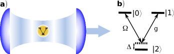
The quantum information is encoded in a superposition of two excited levels $|0\rangle$ and $|1\rangle$. We can operate on this quantum information using two transitions to the intermediate level $|2\rangle$, which is the ground level. The first transition $|1\rangle\leftrightarrow|2\rangle$ is coupled to the cavity mode with a frequency $\omega_{\textrm{cav}}$ and coupling strength $g$. The second transition $|0\rangle\leftrightarrow|2\rangle$ is driven by a classical laser field with a frequency $\omega_{\textrm{L}}$ and coupling strength $\Omega$. The classical laser field and the quantized cavity mode are equally detuned from the corresponding transition frequencies by $\Delta=(E_{0}-E_{2})/\hbar-\omega_{L}$. The V-type level configuration cannot be considered as an ideal memory because, contrary to the $\Lambda$-type system, a qubit is here encoded in a superposition of two excited states, and thus, the time of storage of quantum information is limited by the spontaneous emission. Spontaneous emission rates from levels $|0\rangle$ and $|1\rangle$ we denote by $\gamma_{0}$ and $\gamma_{1}$, respectively. However, new technology shows that it is possible to build devices where the coherent coupling strength is much greater than the spontaneous transition rate englund07:_controlling ; englund10 ; englund12 . In englund07:_controlling the coupling strength $g$ between quantum dot and the microcavity mode is 80 times greater than spontaneous emission rate $\gamma$ for the same transition. Therefore, the V-type level structure can be considered as a short-term memory useful in quantum information processing. Such large values of $g$ compared to $\gamma$ are possible for microcavities since $g$ is inversely proportional to the square of the cavity mode volume. Unfortunately, the cavity decay rate $\kappa$ increases with decreasing the cavity length, and therefore, $\kappa>g$ in englund07:_controlling . Nevertheless, it is reasonable to assume that the finesse of microcavities will be improved in the future and the coherent coupling will dominate all dissipative rates.

The Hamiltonian that describes the interaction of the atom (or the quantum dot) with the cavity field mode is given by

$$H = -\Delta\sigma_{22}+(\Omega\sigma_{02}+ga\sigma_{12}+{\rm{h.c.}})$$ (1)

$$-i\kappa a^{\dagger}a-i\gamma_{0}\sigma_{00}-i\gamma_{1}\sigma_{11}\,,$$

where $\sigma_{ij}=|i\rangle\langle j|$ denote the atomic flip operators and $a$ denotes the annihilation operator of the cavity mode.

III Nonexistence of perfect mapping pulse for V systems

Let us consider the case of the unitary evolution of the system, i.e., we assume that $\kappa$, $\gamma_{0}$ and $\gamma_{1}$ are equal to zero. The quantum information encoded in the atomic state $\alpha|00\rangle+\beta|10\rangle$ has to be mapped perfectly and quickly onto the cavity field state: $\alpha|00\rangle+\beta|01\rangle$. Here, we have denoted a state of the system consisting of the atomic state $|j\rangle$ and the cavity field with $n$ photons by $|jn\rangle$. So, we have to perform quantum operation defined by $|10\rangle\to|01\rangle$ and $|00\rangle\to|00\rangle$. Is it possible to achieve this task using the evolution governed by the Hamiltonian (1)? Let us investigate this problem. The evolution of the state $|10\rangle$ is given by

$$e^{-iHt}|10\rangle = a(t)|10\rangle+b(t)|01\rangle+c(t)|21\rangle\,,$$ (2)

where

$$a(t) = 1-|g|^{2}/(|\Omega|^{2}+|g|^{2})\,f(t)\,,$$

$$b(t) = -\Omega\,g^{*}/(|\Omega|^{2}+|g|^{2})\,f(t)\,,$$

$$c(t) = -ig^{*}/\nu\,e^{i\,\Delta/2\,t}\sin{\nu\,t}\,,$$ (3)

with $\nu=\sqrt{(\Delta/2)^{2}+|\Omega|^{2}+|g|^{2}}$ and

$$f(t) = 1+e^{i\,\Delta/2\,t}(i\Delta/(2\nu)\sin{\nu\,t}-\cos{\nu\,t})\,.$$ (4)

From (III) one can see that the population of the state $|10\rangle$ will be fully transferred to the state $|01\rangle$ if three conditions will be satisfied, i.e., $|g|=|\Omega|$, $\sin{\nu\,t}=0$ and $f(t)=2$. Taking into account two first conditions we can express the third one in the form

$$\cos{(\Delta/2\,t_{\pi})}\cos{\nu\,t_{\pi}} = -1\,.$$ (5)

Equation (5) leads to a discrete set of detunings chimczak08:_fine

$$\Bigg{(}\frac{\Delta}{2\,|g|}\Bigg{)}^{2} = 2\,\frac{\zeta^{2}}{2\zeta+1}\,,$$ (6)

where $\zeta=k/\theta$, $\theta=1,3,5,\dots$ is a natural odd number and $k=0,1,2,3,\dots$ is a non-negative integer. So, the population is fully transferred from the state $|10\rangle$ to $|01\rangle$ if and only if the value of detuning satisfies condition (6) and the operation time $t_{\pi}$ is given by

$$t_{\pi} = 2k\pi/|\Delta|=(\theta+k)\pi/\nu\,.$$ (7)

If we assume that $\Omega=-g\exp(i\Phi)$ then it is seen from (2) and (III) that such a perfect $\pi$ pulse is given by

$$U_{\pi}|10\rangle \equiv e^{-iHt_{\pi}}|10\rangle=e^{i\Phi}|01\rangle\,.$$ (8)

The state-mapping operation requires also that the population of the state $|00\rangle$ has to remain unchanged. In the case of three-level $\Lambda$ systems the state $|00\rangle$ experiences no dynamics. Therefore, in such systems the perfect state-mapping operation (also defined by $|10\rangle\to|01\rangle$ and $|00\rangle\to|00\rangle$) can be easily achieved. The situation, however, is considerably more complicated for three-level V systems. In V systems the time evolution is given by

$$e^{-iHt}|00\rangle = e^{i\Delta/2\,t}\Big{[}(2\nu^{\prime}\cos{\nu^{\prime}\,t}-i\Delta\sin{\nu^{\prime}\,t})|00\rangle$$ (9)

$$-i2\Omega^{*}\sin{\nu^{\prime}\,t}|20\rangle\Big{]}/(2\nu^{\prime})\,,$$

$$e^{-iHt}|20\rangle = e^{i\Delta/2\,t}\Big{[}(2\nu^{\prime}\cos{\nu^{\prime}\,t}+i\Delta\sin{\nu^{\prime}\,t})|20\rangle$$ (10)

$$-i2\Omega\sin{\nu^{\prime}\,t}|00\rangle\Big{]}/(2\nu^{\prime})\,,$$

where $\nu^{\prime}=\sqrt{(\Delta/2)^{2}+|\Omega|^{2}}$. It is worth to mention here that these above equations hold also for $\kappa\neq 0$. During the evolution described by (9) the population of the intermediate state is given by

$$\langle\sigma_{22}\rangle = \frac{4|\Omega|^{2}}{\Delta^{2}+4|\Omega|^{2}}\sin^{2}(\nu^{\prime}t)\,.$$ (11)

The condition $|00\rangle\to|00\rangle$ is fulfilled up to a phase factor if the operation time is given by

$$t_{\pi}^{\prime} = l\,\pi/\nu^{\prime}\,,$$ (12)

where $l=1,2,3,\dots$ is a positive integer. Since the state-mapping operation requires both conditions $|10\rangle\to|01\rangle$ and $|00\rangle\to|00\rangle$, an operation time $t_{\rm{m}}$ has to be equal to  (7) and (12), and the detuning has to satisfy (6). These three conditions lead to a Diophantine equation

$$k^{2}+(\theta+k)^{2} = 2\,l^{2}\,.$$ (13)

It follows from (13) that the numbers $k$ and $(\theta+k)$ should be both odd or both even. However, the numbers $k$ and $(\theta+k)$ will never be both odd or both even, because $\theta$ is always an odd number. Thus, (13) has no solutions in natural numbers $k$, $l$, $\theta$ with $\theta$ odd.

One can see that three-level V systems have important drawback. The fidelity of the state-mapping operation is always reduced by the population of the intermediate level, and therefore the perfect state mapping using single rectangular laser pulse is impossible in three-level V-type systems.

Moreover, it seems likely that there is no prefect state mapping consisting of more than one laser pulse. However, it is hard to prove it because there are infinitely many possible sequences of laser pulses — from two different pulses to series of very many ultra-short pulses as in kowalewska09 .

IV Approximate state mapping

We already know that there is no perfect state-mapping operation in three-level V systems, i.e., $t_{\pi}$ will be never equal to $t_{\pi}^{\prime}$. However, $t_{\pi}$ can be very close to $t_{\pi}^{\prime}$ for some special numbers $k$, $l$, and $\theta$. In such cases it is possible to perform an approximate state-mapping operation with the operation time $t_{\rm{m}}\approx(t_{\pi}+t_{\pi}^{\prime})/2$. Now we investigate if approximate state-mapping operations can satisfy the fidelity requirement of large quantum algorithms. Of course, the fidelity of approximate state-mapping operations is state dependent, and therefore, we need the minimum fidelity taken over all possible input states in our investigation. Since computational speed is also very important, the times of these operations $t_{\rm{m}}$ should be not too long. We have calculated the minimal fidelity of state mapping for all such $k$, $l$ and $\theta$, for which the operation time is shorter than some fixed time limit $200g^{-1}$. We have found that there are only fourteen different state-mapping operations, which can satisfy the fidelity requirement of large quantum algorithms $F\geq 1-10^{-5}$ and take less time than the chosen time limit $200g^{-1}$. We have only fourteen different values of the detuning, which we can choose. The shortest approximate state-mapping operation lasts $109.5g^{-1}$ and is determined by $(k,\theta,l)=(63,17,72)$. So, it is possible to perform the approximate state mapping, but such an approximate state mapping cannot be short and achieve very high fidelity at once.

V Almost perfect state mapping for V systems

The state-mapping operation performed using a single rectangular laser pulse in V-type systems cannot achieve fidelity equal to unity. The population of the intermediate state $|2\rangle$ reduces the fidelity.

Figure 2: Populations of the states $|20\rangle$ (solid line), $|21\rangle$ (dotted line) and $|10\rangle$ (dashed line) during the $\pi$ pulse operation. A non-zero population of the state $|20\rangle$ at the end of the pulse reduces the fidelity. Inset: the $\pi$ pulse. Here we set $g=2\pi\times 10$ MHz.

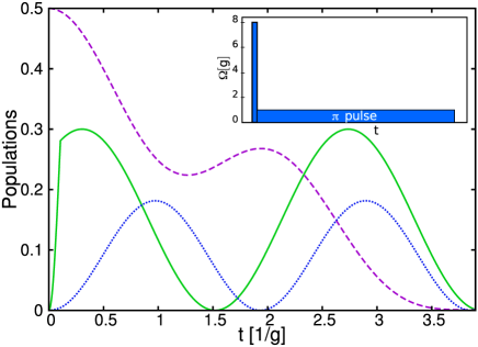
This situation is illustrated in figure 2 — the initial state $(|00\rangle+|10\rangle)/\sqrt{2}$ cannot be perfectly transformed into $(|00\rangle+|01\rangle)/\sqrt{2}$ because of a non-zero population of the state $|20\rangle$ at the end of the pulse. The problem comes from the fact that the states $|10\rangle$ and $|00\rangle$ (which belong to orthogonal subspaces {$|10\rangle$, $|01\rangle$, $|21\rangle$} and {$|00\rangle$, $|20\rangle$}) evolve with noncommensurate frequencies $\nu=\sqrt{(\Delta/2)^{2}+2|g|^{2}}$ and $\nu^{\prime}=\sqrt{(\Delta/2)^{2}+|g|^{2}}$ (for $|\Omega|=|g|$). The operations $|10\rangle\to|01\rangle$ and $|00\rangle\to|00\rangle$ require the $\pi$ pulse and the $2\pi$ pulse, respectively. Since $\nu$ and $\nu^{\prime}$ are noncommensurate, the duration times of these pulses are always different, and therefore, there is no rectangular pulse which can perform operations $|10\rangle\to|01\rangle$ and $|00\rangle\to|00\rangle$ simultaneously.

We can omit this problem shifting the evolution in the subspace {$|00\rangle$, $|20\rangle$} with respect to the evolution in the subspace {$|10\rangle$, $|01\rangle$, $|21\rangle$} before performing the perfect $\pi$ pulse operation. By ’shifting the evolution’ we mean that the state $|10\rangle$ experiences no dynamics while the state $|00\rangle$ is transformed into such a special state $|\Phi_{\eta}\rangle=\eta_{0}|00\rangle+\eta_{1}|20\rangle$ that $U_{\pi}|\Phi_{\eta}\rangle=|00\rangle$.

Figure 3: Populations of the states $|20\rangle$ (solid line), $|21\rangle$ (dotted line) and $|10\rangle$ (dashed line) during the two-stage state-mapping protocol. At the end these three populations are close to zero, and thus, the fidelity can be close to one. Inset: the pulses sequence.

The main idea of such a two-stage state-mapping protocol is illustrated in figure 3. Thus, in the first stage of this protocol we need an operation, which changes only the state that belongs to the subspace {$|00\rangle$, $|20\rangle$} and leaves the state belonging to the other subspace unchanged.

This needed operation is just the intense laser pulse operation. It is clearly seen from equations (2), (III) and (9) that when the laser pulse is very intensive $|\Omega|\gg|g|$ then $a(t)\approx 1$, and therefore, the state $|10\rangle$ experiences almost no dynamics while the population of the state $|00\rangle$ oscillates with a very high frequency. In the following, we will assume that $a(t)=1$ for $|\Omega|\gg|g|$. Since we need the fidelity greater than $1-10^{-5}$, we have to estimate the error $\epsilon=1-|a(t)|^{2}$ introduced by this approximation. From (III) we see that

$$|a(t)|^{2} > 1-\frac{|g|^{2}}{(|\Omega|^{2}+|g|^{2})}\,2\,{\rm{Re}}({f(t_{1})})\,,$$ (14)

where ${\rm{Re}}({f(t)})\leq 2$, and thus the probability that the system will be found in other state than $|10\rangle$ is limited by

$$\epsilon < \frac{4\,|g|^{2}}{|\Omega|^{2}+|g|^{2}}\quad<\quad\Big{(}\frac{2\,|g|}{|\Omega|}\Big{)}^{2}\,.$$ (15)

Therefore, $|\Omega/g|>633$ is necessary to get the error probability smaller than $10^{-5}$.

The effect of this operation is given by $U_{1}(t_{1})|10\rangle=|10\rangle$ and

$$U_{1}(t_{1})|00\rangle = e^{i\Delta/2\,t_{1}}\big{[}(2\nu^{\prime}_{1}\cos{\nu^{\prime}_{1}\,t_{1}}-i\Delta\sin{\nu^{\prime}_{1}\,t_{1}})|00\rangle$$ (16)

$$-i2\Omega^{*}\sin{\nu^{\prime}_{1}\,t_{1}}|20\rangle\big{]}/(2\nu^{\prime}_{1})\,,$$

where $\nu_{1}^{\prime}=\sqrt{(\Delta/2)^{2}+|\Omega|^{2}}$. From (16) it is seen that we can set arbitrary populations of the states $|00\rangle$ and $|20\rangle$ for $|\Omega|\gg|\Delta|$. It is also seen that we can easily give an arbitrary phase shift to the state $|20\rangle$ with respect to the state $|00\rangle$ just by setting proper argument of $\Omega=\Omega_{1}\exp(i\phi_{\Omega})$, where $\Omega_{1}=|\Omega|$. So we can always produce the state $|\Phi_{\eta}\rangle$ for large enough $\Omega_{1}$.

We can calculate amplitudes $\eta_{0}$ and $\eta_{1}$ by premultiplying $U_{\pi}|\Phi_{\eta}\rangle=|00\rangle$ by $U_{\pi}^{-1}=e^{iHt_{\pi}}$. We also assume that in the second stage of the protocol, i.e., during the perfect $\pi$ pulse we change the intensity and the phase of the laser field that $\Omega=-g\exp(i\Phi)$. In this way we get

$$|\Phi_{\eta}\rangle = e^{-i\Delta/2\,t_{\pi}}\big{[}(2\nu_{\pi}^{\prime}\cos{\nu_{\pi}^{\prime}\,t_{\pi}}+i\Delta\sin{\nu_{\pi}^{\prime}\,t_{\pi}})|00\rangle$$ (17)

$$-ie^{-i\Phi}2g^{*}\sin{\nu_{\pi}^{\prime}\,t_{\pi}}|20\rangle\big{]}/(2\nu_{\pi}^{\prime})\,,$$

where $\nu^{\prime}_{\pi}=\sqrt{(\Delta/2)^{2}+|g|^{2}}$. A comparison of the moduli of the amplitudes (16) and (17) leads to

$$t_{1} = \arccos{\Big{(}1-2\frac{|g|^{2}\nu_{1}^{\prime 2}}{\Omega_{1}^{2}\nu_{\pi}^{\prime 2}}(\sin{\nu^{\prime}_{\pi}\,t_{\pi}})^{2}}\Big{)}/(2\nu^{\prime}_{1})\,.$$ (18)

In order to find the proper argument of $\Omega$ we write (16) and (17) in terms of the moduli and the arguments of $\eta_{0}$ and $\eta_{1}$

$$U_{1}|00\rangle = \big{(}|\eta_{0}|e^{i\theta_{0}}|00\rangle+|\eta_{1}|e^{i\theta_{1}}|20\rangle\big{)}e^{i\Delta/2\,t_{1}}\,,$$ (19)

$$|\Phi_{\eta}\rangle = \big{(}|\eta_{0}|e^{i\phi_{0}}|00\rangle+|\eta_{1}|e^{i\phi_{1}}|20\rangle\big{)}e^{-i\Delta/2\,t_{\pi}}\,,$$ (20)

where

$$|\eta_{1}| = \frac{|g|}{\nu_{\pi}^{\prime}}|\sin{\nu_{\pi}^{\prime}\,t_{2\pi}}|\,,$$

$$|\eta_{0}| = \big{(}|g|^{2}\cos^{2}{\nu_{\pi}^{\prime}\,t_{\pi}}+\Delta^{2}/4\big{)}^{1/2}/\nu^{\prime}_{\pi}\,.$$ (21)

The arguments of phase factors are given by

$$\phi_{1}=\left\{\begin{array}[]{l}\frac{3}{2}\pi-\Phi-\phi_{g}\,,\quad{\rm{if}}\quad\sin{\nu_{\pi}^{\prime}\,t_{\pi}}>0\,,\\ \frac{1}{2}\pi-\Phi-\phi_{g}\,,\quad{\rm{if}}\quad\sin{\nu_{\pi}^{\prime}\,t_{\pi}}<0\end{array}\right.$$ (24)

and

$$\phi_{0} = \arctan\Big{(}\frac{\Delta}{2\nu_{\pi}^{\prime}}\tan{\nu_{\pi}^{\prime}\,t_{\pi}}\Big{)}+k^{\prime}\pi\,,$$

$$\theta_{0} = -\arctan{\Big{(}\frac{\Delta}{2\nu^{\prime}_{1}}\tan{\nu^{\prime}_{1}t_{1}}\Big{)}}\,,$$

$$\theta_{1} = \frac{3}{2}\pi-\phi_{\Omega}\,,$$ (25)

where $\phi_{g}$ is the argument of $g$ and $k^{\prime}$ is 0 or even for $\cos{\nu_{\pi}^{\prime}\,t_{\pi}}>0$ and odd for $\cos{\nu_{\pi}^{\prime}\,t_{\pi}}<0$.

Now it is easy to check that if we chose such $\phi_{\Omega}$ that the condition $\phi_{0}-\phi_{1}+3\pi/2-\phi_{\Omega}-\theta_{0}=2\,l^{\prime}\,\pi$ is fulfilled then $U_{1}|00\rangle=e^{i\Theta}|\Phi_{\eta}\rangle$, where $\Theta=\Delta/2\,(t_{1}+t_{\pi})+\theta_{0}-\phi_{0}$ and $l^{\prime}$ is an integer.

VI The state-mapping protocol

The protocol that is able to achieve fidelity as close to unity as it is needed consists of two stages: (A) the evolution-shift stage, and (B) the $\pi$ pulse stage. Initially, the quantum system is prepared in the state

$$|\psi_{0}\rangle = \alpha|10\rangle+\beta|00\rangle\,.$$ (26)

For simplicity, we assume here, and in the following, that $g$ is a real positive number.

VI.1 The evolution-shift stage

The goal of this stage is to transform the state $|00\rangle$ into $|\Phi_{\eta}\rangle$ without changing the state $|10\rangle$. To this end, we turn the laser on for the time $t_{1}$, given by (18). The laser has to be set in such a way that $\Omega=\Omega_{1}\exp(i\phi_{\Omega})$ with $\phi_{\Omega}=\Delta/2\,(t_{1}+t_{\pi})+m\,\pi$, where $m$ is 0 or even for $\sin{\nu_{\pi}^{\prime}\,t_{\pi}}>0$ and odd for $\sin{\nu_{\pi}^{\prime}\,t_{\pi}}<0$. The intensity of the laser light has to be great enough to satisfy the condition $\Omega_{1}\gg g$. This operation is described by $U_{1}|10\rangle=|10\rangle$ and $U_{1}|00\rangle=e^{i\Theta}|\Phi_{\eta}\rangle$, and therefore, at the end of this stage, the system state is given by

$$|\psi_{1}\rangle = \alpha|10\rangle+\beta e^{i\Theta}|\Phi_{\eta}\rangle\,.$$ (27)

VI.2 The $\pi$ pulse stage

In the second stage of this protocol we change the intensity of the laser light to satisfy condition $\Omega=-g\exp(i\Phi)$ and we keep the laser on for the time $t_{\pi}$. The $\pi$ pulse operation is described by $U_{\pi}|10\rangle=e^{i\Phi}|01\rangle$ and $U_{\pi}|\Phi_{\eta}\rangle=|00\rangle$. So, after this $\pi$ pulse operation the system state is given by

$$|\psi_{f}\rangle = \alpha e^{i\Phi}|01\rangle+\beta e^{i\Theta}|00\rangle\,.$$ (28)

If we set $\Phi=\Theta$ then the protocol ends up with the state

$$|\psi_{f}\rangle = \alpha|01\rangle+\beta|00\rangle$$ (29)

$$= |0\rangle_{\rm{dot}}\otimes(\alpha|1\rangle_{\rm{cav}}+\beta|0\rangle_{\rm{cav}})\,.$$

The condition $\Phi=\Theta$ leads to $\Phi=\Delta/2\,(t_{1}+t_{\pi})+\theta_{0}-\phi_{0}$.

VII Validity of the rotating wave approximation

Results obtained using (1) show that the fidelity of the state-mapping protocol tends to unity for large $|\Omega|$. However, we have to keep in mind that the Hamiltonian given by (1) describes the quantum system composed of the V-type atom or atom-like structure and the cavity in the rotating-wave approximation (RWA). This means that we cannot set $|\Omega|$ too high because (1) will be unreliable book_petruccione . The careful choice of $|\Omega|$ is especially important in the performing of state mapping with a very high fidelity. Therefore, we have to take into account in our considerations counter-rotating terms which are neglected in RWA. The Hamiltonian without RWA is given by

$$H = -\Delta\sigma_{22}+(\Omega\sigma_{02}+ga\sigma_{12}$$ (30)

$$+\Omega\sigma_{12}e^{i(\omega_{\rm{L}}+\omega_{\rm{cav}})t}+ga\sigma_{20}e^{-i(\omega_{\rm{L}}+\omega_{\rm{cav}})t}+{\rm{h.c.}})$$

$$-i\kappa a^{\dagger}a-i\gamma_{0}\sigma_{00}-i\gamma_{1}\sigma_{11}\,.$$

Here, we have assumed that the classical laser field and the quantized cavity mode field are $\sigma^{-}$ and $\sigma^{+}$ polarized, respectively. We can estimate the error introduced by the counter-rotating terms using (30) and time-dependent perturbation theory. The quantum system, which is initially prepared in the state $|10\rangle$ should remain in this state after the first stage. Assuming that $|\Omega|,\,|\Delta|\ll\omega_{\rm{L}}+\omega_{\rm{cav}}$ and $|\Omega|\gg|g|$, the probability that it will be found in other state can be roughly approximated by

$$\epsilon = \epsilon_{1}+\epsilon_{2}<\Big{(}\frac{2\,|g|}{|\Omega|}\Big{)}^{2}+\Big{(}\frac{2\,|\Omega|}{\omega_{\rm{L}}+\omega_{\rm{cav}}}\Big{)}^{2}\,.$$ (31)

One can see that the first term of (31), which represents the error introduced by terms $ga\sigma_{12}+{\rm{h.c.}}$, is in agreement with (15). The second term represents the error introduced by the counter-rotating terms.

Now it is easy to check that RWA is justified for atoms. For atoms, typically $g/2\pi$ is of order 10 MHz and $\omega_{\rm{L}}/2\pi\approx\omega_{\rm{cav}}/2\pi\approx 3.8\times 10^{8}$ MHz, so $\epsilon_{2}$ is smaller than $10^{-6}$ up to $|\Omega|/g\approx 3\times 10^{4}$. The situation is more complicated for quantum dots. We will consider the case of quantum dots later.

VIII The numerical tests of the state-mapping protocol

Let us see capabilities of the state-mapping protocol and check the derived formulas using numerical computations. First, we examine the protocol for a great value of the detuning $|\Delta|\gg g$. Here, and in the following, we set $g=2\pi\times 10$ MHz. For $(k,\theta)=(25,1)$ and $\Omega_{1}/g=100$ we obtain $\Delta/g=9.90148$, $(t_{1},t_{\pi})=(2.0\times 10^{-3},15.864)g^{-1}$, $(\phi_{\Omega},\Phi)=(0.01,4.696)$ and $F>1-2\times 10^{-6}$. It is seen that the total time of the protocol is much shorter than the time of the shortest approximate state-mapping solution. It is also worth to note that $t_{1}\ll t_{\pi}$, which means that the state-mapping protocol for V-type systems is almost as fast as state mapping in $\Lambda$-type systems. The fidelity is very close to one, so it is almost as high as fidelity of state mapping in $\Lambda$-type systems. According to (15) we can increase the fidelity. The fidelity of the state-mapping protocol should tend to unity as $\Omega$ becomes large. In order to check it we repeat these calculation for $\Omega_{1}/g=1000$ and we obtain $(t_{1},t_{\pi})=(1.993\times 10^{-4},15.8642)g^{-1}$, $(\phi_{\Omega},\Phi)=(0.001,4.6966)$ and $F>1-2\times 10^{-8}$. As expected from (15), the error probability is proportional to $(g/\Omega_{1})^{2}$.

We can come to the same conclusions simulating the state-mapping protocol for small values of $\Delta$. For example, $(k,\theta)=(1,1)$ and $\Omega_{1}/g=100$ lead to $\Delta/g=1.633$, $(t_{1},t_{\pi})=(8.5\times 10^{-3},3.847)g^{-1}$, $(\phi_{\Omega},\Phi)=(0.007,4.319)$ and $F>1-7\times 10^{-5}$. It is seen that the perfect $\pi$ pulse is faster for small values of $\Delta$. It is also seen that the fidelity is smaller than in case of large $\Delta$. This, however, is not a problem. We can always increase the fidelity by increasing $\Omega_{1}/g$. For $\Omega_{1}/g=1000$ we obtain $\Delta/g=1.633$, $(t_{1},t_{\pi})=(8.47\times 10^{-4},3.8476)g^{-1}$, $(\phi_{\Omega},\Phi)=(0.0007,4.321)$ and $F>1-5\times 10^{-7}$.

IX The effect of a non-zero $\kappa$ on the protocol

The evolution of the state of real optical cavities is not unitary because of absorption of photons in mirrors. In some of devices photons can also leak out of the cavity through a semitransparent mirror. Such a photon leakage is very important when quantum information encoded in the photonic state of the cavity has to be transferred to a distant quantum system. We can take into account these photon losses assuming that cavity decay rate $\kappa$ is greater than zero. Let us now consider the effect of non-zero $\kappa$ on operations needed by the state-mapping protocol, i.e., $|10\rangle\to|01\rangle$ and $|00\rangle\to|00\rangle$.

As mentioned above, the evolution of the system prepared initially in the state $|00\rangle$ is independent of $\kappa$. Hence, the time of the operation $|00\rangle\to|00\rangle$ is still given by (12). However, a non-zero $\kappa$ changes the evolution of the system prepared initially in the state $|10\rangle$. For small values of $\kappa$, we can find a good approximation to this evolution applying the first order perturbation theory. In order to write the expressions in a more compact form, we assume that $|\Delta|\gg g\gg\kappa$. Then the expansion parameter can be well approximated by $\eta=\kappa|\Delta|/(4g^{2})\ll 1$ and the evolution of the system is quite well described by

$$e^{-iHt}|10\rangle = a_{\kappa}(t)|10\rangle+b_{\kappa}(t)|01\rangle+c_{\kappa}(t)|21\rangle\,,$$ (32)

where

$$a_{\kappa}(t) = e^{-\kappa t/2}\big{[}e^{(i\omega_{+}-\kappa\xi_{+})t/2}\omega_{-}(1-i2\eta\xi_{-})/(8\nu)-i\eta\epsilon$$

$$+e^{-(i\omega_{-}+\kappa\xi_{-})t/2}\omega_{+}(1+i2\eta\xi_{+})/(8\nu)+1/2\big{]}\,,$$

$$b_{\kappa}(t) = -e^{i\Phi}e^{-\kappa t/2}\big{[}e^{(i\omega_{+}-\kappa\xi_{+})t/2}\omega_{-}/(8\nu)-1/2$$

$$+e^{-(i\omega_{-}+\kappa\xi_{-})t/2}\omega_{+}/(8\nu)\big{]}\,,$$

$$c_{\kappa}(t) = \frac{g}{2\nu}e^{(i\Delta-\kappa)t/2}\big{(}e^{-(i\nu+\kappa\xi_{-}/2)t}-e^{(i\nu-\kappa\xi_{+}/2)t}\big{)}\,.$$

In (IX), $\omega_{\pm}=2\nu\pm\Delta$ and $\epsilon={\rm{sign}}(\Delta)$ and $\xi_{\pm}=H(\pm\Delta)$, where $H(t)$ denotes the Heaviside function.

From (IX), it is easy to check that the population of the intermediate state $|c_{\kappa}|^{2}$ is greater than zero for $t>0$. This means that the state-mapping operation cannot be perfect for $\kappa>0$.

Figure 4: The population of state $|21\rangle$ computed numerically versus time for a non-zero cavity decay rate. This population reduces the fidelity of the state mapping. The parameters are $(\Delta,\Omega,\kappa,\gamma_{0},\gamma_{1})/g=(4,1,0.1,0,0)$, where $g=2\pi\times 10$ MHz.

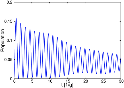
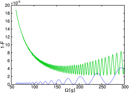
In figure 4 we plot the population of state $|21\rangle$ for quite large value of $\kappa$ to show that this population reaches a local minimum periodically, but does not reach zero. We can infer two consequences from this. First, a very high fidelity is possible only for very small $\kappa t$. Second, although we can only approximate the operation $|10\rangle\to|01\rangle$, this approximation can be quite good if we use the oscillatory behaviour of $|c_{\kappa}|^{2}$ to minimize it. It is interesting that the local minima of $|c_{\kappa}|^{2}$ are almost independent of $\kappa$. So, to a good approximation, this population takes minimum values at

$$t=m^{\prime}\pi/\nu\,,$$ (34)

where $m^{\prime}$ is a positive integer.

Second important difference in the operation $|10\rangle\to|01\rangle$ between cases when the damping is present and when is not is the time of this operation. In order to get an approximated formula for the $\pi$ pulse, we need further approximations. Recalling that $|\Delta|\gg g\gg\kappa$, we drop all small terms and as a result we eliminate the state $|21\rangle$ from the evolution. Expressions for amplitudes obtained in this way are less precise, but much simpler

$$a_{\kappa}(t) = e^{-i\epsilon\delta t}e^{-\kappa t/2}\big{(}\cos{\delta t}+2\eta\sin{\delta t}\big{)}\,,$$

$$b_{\kappa}(t) = i\epsilon e^{i\Phi}e^{-i\epsilon\delta t}e^{-\kappa t/2}\sin{\delta t}\,,$$

$$c_{\kappa}(t) = 0\,,$$ (35)

where $\delta=(2\nu-|\Delta|)/4\approx g^{2}/|\Delta|$. The $\pi$ pulse requires $a_{\kappa}(t)=0$, and therefore the time of this pulse is given by

$$t_{\pi}(\kappa) = \delta^{-1}\big{[}k^{\prime\prime}\pi-\arctan\big{(}(2\eta)^{-1}\big{)}\big{]}\,,$$ (36)

where $k^{\prime\prime}=1,2,3,\dots$ Using the linear approximation, we can also express $t_{\pi}(\kappa)$ in the form

$$t_{\pi}(\kappa) = \theta\pi/(2\delta)+2\eta\delta^{-1}=t_{\pi}(0)+2\eta\delta^{-1}\,,$$ (37)

where $t_{\pi}(0)$ is given by (7). This $\pi$ pulse is close to be perfect when the population of the intermediate state takes minimum value at the end of this pulse. Therefore, the time given by (37) has to be equal to that given by (34). This is possible only for the fine tuned values of the detuning

$$|\Delta(\kappa)| = |\Delta(0)|\Big{(}1-\frac{2\eta}{\theta\pi}\Big{)}\,,$$ (38)

where $\Delta(0)$ is given by (6).

The $\pi$ pulse operation for non-zero $\kappa$ can be approximated by $U_{\pi}|10\rangle=e^{i(\Phi-\epsilon 2\eta)}e^{-\kappa t_{\pi}/2}|01\rangle$ and $U_{\pi}|\Phi_{\eta}\rangle=|00\rangle$. Therefore, after the second stage of the protocol the unnormalized state of the system is given by

$$|\widetilde{\psi}_{f}\rangle = \alpha e^{i(\Phi-\epsilon 2\eta)}e^{-\kappa t_{\pi}/2}|01\rangle+\beta e^{i\Theta}|00\rangle\,.$$ (39)

Now it is useful to set $\Phi$, which satisfies the condition $\Theta=\Phi-\epsilon 2\eta$. This leads to

$$\phi_{\Omega} = \Delta/2\,(t_{1}+t_{\pi})+m\,\pi+\epsilon 2\eta\,,$$

$$\Phi = \Delta/2\,(t_{1}+t_{\pi})+\theta_{0}-\phi_{0}+\epsilon 2\eta\,.$$ (40)

Then at the end of the protocol we obtain

$$|\psi_{f}\rangle = {\cal{N}}(\alpha e^{-\kappa t_{\pi}/2}|01\rangle+\beta|00\rangle)\,,$$ (41)

where ${\cal{N}}=(|\alpha|^{2}e^{-\kappa t_{\pi}}+|\beta|^{2})^{-1/2}$ is the normalization factor. Observe that for non-zero values of $\kappa$ the state mapping is not perfect because of the damping factor $e^{-\kappa t_{\pi}/2}$. We can achieve high fidelity for small enough values of $\kappa t_{\pi}$ only.

Using (37), (38), (IX) and (18) we find that the minimal fidelity exceeds the value $1-10^{-5}$ for $(\Delta,\Omega_{1},\kappa)/g=(9.890\,55,1000,7\times 10^{-4})$, $(t_{1},t_{\pi})=(2\times 10^{-4},15.882)g^{-1}$ and $(\phi_{\Omega},\Phi)=(0.008,4.696)$. More considerable value of $\kappa$ we can set for small values of $\Delta$, because then the $\pi$ pulse is faster and $\kappa t_{\pi}$ smaller. The formulas (37), (38) and (IX) work properly only when $|\Delta|\gg g\gg\kappa$ and $\eta\ll 1$. However, we can use these formulas to calculate the initial starting point and use it in a numerical optimization. In this way we find that we can achieve $F>1-10^{-5}$ for $(\Delta,\Omega_{1},\kappa)/g=(1.630,1000,2.6\times 10^{-3})$, $(t_{1},t_{\pi})=(8.48\times 10^{-4},3.85)g^{-1}$ and $(\phi_{\Omega},\Phi)=(-0.001,4.32)$. We cannot set larger values of $\kappa$ because $\kappa t_{\pi}$ is to large to achieve $F>1-10^{-5}$.

X The influence of spontaneous emission from excited states on the protocol

So far, we have assumed that spontaneous emission decay rates $\gamma_{0}$ and $\gamma_{1}$ are equal to zero. Let us now relax this assumption and investigate the influence of $\gamma_{0}$ and $\gamma_{1}$ on state-mapping operations. It seems obvious that the fidelity of state mapping decreases with increasing $\gamma_{0}$ and $\gamma_{1}$. Sometimes even a small value of the spontaneous decay rate can considerably decrease the fidelity or the success probability chimczak02:_effect . Thus, it may be surprising that non-zero spontaneous emission decay rates can improve state-mapping operations. The reason is that field and atomic damping act in a sense in opposite directions.

Figure 5: The population of the state $|21\rangle$ as a function of time for the same parameters as in figure 4, but for ($\gamma_{0},\gamma_{1})/g=(0.05,0.05)$. For non-zero values of $\gamma_{0}$ and $\gamma_{1}$ this unwanted population again approaches zero periodically.

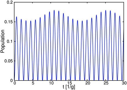
Figure 5 shows that the periodic behaviour of the system lost due to non-zero $\kappa$ can be partially recovered by non-zero $\gamma_{0}$ and $\gamma_{1}$. The unwanted population of the state $|21\rangle$ again approaches zero periodically. The same effect can be also observed in the $\Lambda$-type system chimczak08:_fine . This is one of rare examples of a decay process demonstrating its usefulness in quantum-state engineering. However, it should be noted that the atomic damping mechanism plays this constructive role only when we are able to distinguish and reject unsuccessful cases of state-mapping operations, where spontaneous emissions take place. Fortunately, in V-type systems the quantum system is in the auxiliary level $|2\rangle$ after spontaneous emission, and therefore, it is easy to check whether the spontaneous emission takes place or not.

The atomic damping is responsible for one more surprise — the V-type system can be better than the $\Lambda$-type system for the state mapping. The perfect $\pi$ pulse operation for non-zero $\kappa$, $\gamma_{0}$ and $\gamma_{1}$ can be approximated by $U_{\pi}|10\rangle=e^{i(\Phi-\epsilon 2\eta)}e^{-(\kappa+\gamma_{0}+\gamma_{1})t_{\pi}/2}|01\rangle$ and $U_{\pi}|\Phi_{\eta}\rangle=e^{-\Gamma t_{\pi}}|00\rangle$, where $\Gamma$ is an effective damping rate. If $|\Delta|\gg g\gg\kappa$ and $\eta\ll 1$ then $\Gamma\approx\gamma_{0}$. In this case, at the end of the protocol the unnormalized state of the system is given by

$$|\widetilde{\psi}_{f}\rangle = \alpha e^{-(\kappa+\gamma_{0}+\gamma_{1})t_{\pi}/2}|01\rangle+\beta e^{-\gamma_{0}t_{\pi}}|00\rangle\,.$$ (42)

The normalized system state in the V-type system is given by

$$|\psi_{f}\rangle = {\cal{N^{\prime}}}(\alpha e^{-(\kappa-\gamma_{0}+\gamma_{1})t_{\pi}/2}|01\rangle+\beta|00\rangle)\,,$$ (43)

while the normalized system state in the $\Lambda$-type system is almost independent of $\gamma$ and can be well approximated by

$$|\psi_{f}\rangle = {\cal{N}}(\alpha e^{-\kappa t_{\pi}/2}|01\rangle+\beta|00\rangle)\,.$$ (44)

A comparison of (43) with (44) shows that the damping factor in the V-type system can be closer to one than the damping factor in the $\Lambda$-type system in the case of $\gamma_{0}>\gamma_{1}$ and large detunings. Since the damping factor has significant influence on the fidelity for considerable values of $\kappa$, the fidelity of the state mapping in V-type systems is higher in this case than in $\Lambda$-type systems. In (43) ${\cal{N^{\prime}}}=(|\alpha|^{2}e^{-(\kappa-\gamma_{0}+\gamma_{1})t_{\pi}}+|\beta|^{2})^{-1/2}$.

Now let us use atomic decay to increase $\kappa$ in the state-mapping protocol without decreasing the fidelity. We want $\kappa$ as large as possible because for real cavities it takes considerable values. The state-mapping protocol, for which the minimal fidelity exceeds $1-10^{-5}$, can be performed for $(\Delta,\Omega_{1},\kappa,\gamma_{0},\gamma_{1})/g=(9.8568,1000,1.7\times 10^{-3},1.7\times 10^{-3},7\times 10^{-4})$, $(t_{1},t_{\pi})=(1.98\times 10^{-4},15.932)g^{-1}$ and $(\phi_{\Omega},\Phi)=(-0.006,4.696)$. Even larger value of $\kappa$ can be set for small $\Delta$. Using numerical calculations, we have found that $F>1-10^{-5}$ for $(\Delta,\Omega_{1},\kappa,\gamma_{0},\gamma_{1})/g=(1.619,1000,4.9\times 10^{-3},9.2\times 10^{-3},2\times 10^{-3})$, $(t_{1},t_{\pi})=(8.44\times 10^{-4},3.861)g^{-1}$ and $(\phi_{\Omega},\Phi)=(-0.01,4.32)$.

It is worth to note that it is possible to set $\kappa/g$ larger than $4.9\times 10^{-3}$ with $F>1-10^{-5}$. The main obstacle to achieve such high fidelity for large cavity decay rates is the damping factor in (43). We can overcome this obstacle in the class of algorithms, in which the damping factor is compensated for ShiBiao08 ; chimczak09_nonmax . In this way we can get $F>1-10^{-5}$ for $(\Delta,\Omega_{1},\kappa,\gamma_{0},\gamma_{1})/g=(1.613,1000,1.8\times 10^{-2},9\times 10^{-3},9\times 10^{-3})$, $(t_{1},t_{\pi})=(8.44\times 10^{-4},3.87)g^{-1}$ and $(\phi_{\Omega},\Phi)=(-0.009,4.31)$.

XI The state-mapping protocol in quantum dot systems

A typical range of $g/2\pi$ in quantum dot-cavity systems is $8$ to $38$ GHz englund07:_controlling ; winger08 ; englund10 ; englund12 , so the coupling strength in quantum dot systems is three orders of magnitude larger than in atom-cavity systems. Since the state-mapping protocol needs $|\Omega|\gg g$ in the first stage, counter-rotating terms become important and cannot be neglected. One can check using (31) that for the excitonic wavelength of reinhard2012strongly $\lambda=937.25$ nm ($\omega_{\rm{L}}/2\pi\approx\omega_{\rm{cav}}/2\pi\approx 3.2\times 10^{5}$ GHz) there is no such $|\Omega|$ that $\epsilon<10^{-5}$.

Figure 6: The effect of the counter-rotating terms on the fidelity for small value of $\Delta$ (solid line) and for considerable value of $\Delta$ (dotted line).

It is seen in figure 6 that for $g=2\pi\times 10$ GHz and small value of the detuning $\Delta/g=1.633$ ($(k,\theta)=(1,1)$) we obtain the fidelity, which does not satisfy the requirement of large quantum algorithms, though it is still very high.

Fortunately, $\epsilon_{1}$ can be reduced also by increasing $\Delta$. From (14) it is seen that $\epsilon_{1}$ is proportional to ${\rm{Re}}({f(t_{1})})$, which tends to 0 as $\Delta\to\infty$. Figure 6 shows that for large enough $\Delta$ it is possible to perform the state-mapping protocol with $F\geq 1-10^{-5}$ by setting moderate value of $\Omega_{1}$. We have obtained $F>1-2\times 10^{-6}$ for $g=2\pi\times 10$ GHz, $(k,\theta)=(60,1)$ and $\Omega_{1}/g=62$ (which lead to $\Delta/g=15.4278$, $(t_{1},t_{\pi})=(2.08\times 10^{-3},24.435)g^{-1}$ and $(\phi_{\Omega},\Phi)=(0.016,4.705)$). It is possible to satisfy the requirement of large quantum algorithms even in the presence of field and atomic damping. The state mapping with the minimal fidelity equal to $1-7\times 10^{-6}$ can be performed for $(\Delta,\Omega_{1},\kappa,\gamma_{0},\gamma_{1})/g=(15.4141,62,3.4\times 10^{-4},3.7\times 10^{-4},3.5\times 10^{-4})$, $(t_{1},t_{\pi})=(2.08\times 10^{-3},24.457)g^{-1}$ and $(\phi_{\Omega},\Phi)=(0.021,4.706)$.

It is worth to mention here that quantum optimal control theory khaneja01time ; schmidt11optimal makes it possible to manipulate spins very fast and with high fidelity in two level systems beyond the RWA regime scheuer14precise . This is all what is needed in the first stage of the state-mapping protocol performed in quantum dot-cavity systems. Therefore it is possible that the presented results may be improved by using optimal control theory.

XII Experimental feasibility of the protocol

Finally, we shortly discuss the realizability of the state-mapping protocol in a quantum system consisted of a quantum dot placed in a photonic crystal cavity, like in reinhard2012strongly . A neutral exciton $X^{0}$ eigenstates naturally form a three-level V-type system. Let us set experimentally achievable coupling strength $g=2\pi\times 10$ GHz and the exciton decay rate $\hbar\gamma=0.66\mu{\rm{eV}}$ ($\gamma/g=0.016$) reinhard2012strongly . Let us also assume that the damping factor is compensated for. Then we can obtain high fidelity $F>1-1.3\times 10^{-4}$ for $(\Delta,\Omega_{1},\kappa,\gamma_{0},\gamma_{1})/g=(1.599,166,3.2\times 10^{-2},1.6\times 10^{-2},1.6\times 10^{-2})$, $(t_{1},t_{\pi})=(5.04\times 10^{-3},3.888)g^{-1}$ and $(\phi_{\Omega},\Phi)=(-0.0025,4.30)$. Note that the protocol time is short compared with $\gamma^{-1}$ of reinhard2012strongly . However, the protocol time is comparable to $\gamma^{-1}_{\rm{deph}}$ of reinhard2012strongly , where $\gamma_{\rm{deph}}$ is the exciton pure dephasing rate. Moreover, as mentioned above, the value of the cavity decay rate required by the protocol is demanding for present technology. In our numerical calculations we have chosen value $\kappa/g=3.2\times 10^{-2}$, which is 40 times smaller than that of reinhard2012strongly .

XIII Conclusions

I have shown that V-type quantum systems consisting of an atom or atom-like structure and optical cavity have important drawback — quantum information stored in a superposition of two excited states cannot be exactly mapped onto cavity mode state using a single rectangular laser pulse. The fidelity of such a state mapping is always reduced by the population of the intermediate ground state. However, I have found that there exists a two-stage state-mapping protocol for V-type systems, which performs the state-mapping operation almost perfectly, i.e., the fidelity tends to unity with increasing the intensity of the laser light in the first stage of the protocol. Since the first stage is ultra-short, this protocol is almost as fast as state mapping performed in $\Lambda$-type quantum systems. The protocol time is short compared with $\gamma^{-1}$ of englund07:_controlling . I have also investigated the influence of field and atomic damping on this protocol. I have shown that the atomic decay can be useful in the state-mapping protocol — it can suppress unwanted effects of the cavity decay. The atomic decay partially recovers the periodic behaviour of the system and can make the damping factor close to one. Surprisingly, in the limit of large detunings the state-mapping protocol for V-type systems can achieve higher fidelity than the state mapping for $\Lambda$-type systems due to the atomic damping.