Eguchi-Kawai reduction with one flavor of adjoint Möbius fermion

Abstract

We study the single site lattice gauge theory of $SU(N)$ coupled to one Dirac flavor of fermion in the adjoint representation. We utilize Möbius fermions for this study, and accelerate the calculation with graphics processing units (GPUs). Our Monte Carlo simulations indicate that for sufficiently large inverse ’t Hooft coupling $b=1/g^{2}N$, and for $N\leq 10$ the distribution of traced Polyakov loops has “fingers” that extend from the origin. However, in the massless case the distribution of eigenvalues of the untraced Polyakov loop becomes uniform at large $N$, indicating preservation of center symmetry in the thermodynamic limit. By contrast, for a large mass and large $b$, the distribution is highly nonuniform in the same limit, indicating spontaneous center symmetry breaking. These conclusions are confirmed by comparing to the quenched case, as well as by examining another observable based on the average value of the modulus of the traced Polyakov loop. The result of this investigation is that with massless adjoint fermions center symmetry is stabilized and the Eguchi-Kawai reduction should be successful; this is in agreement with most other studies.

I Introduction

Eguchi-Kawai reduction Eguchi and Kawai (1982) is an attractive idea in which a gauge theory becomes spacetime volume independent for a large number of colors $N$ in a $U(N)$ or $SU(N)$ gauge theory. Originally this was shown by demonstrating that the Schwinger-Dyson equations (loop equations) for suitably defined Wilson loops are equivalent in two lattice Yang-Mills theories at large $N$: a model with an infinite number of sites in all four spacetime dimensions and a model with a single site. However, after the appearance of Eguchi and Kawai (1982) it was rapidly shown that there is a phase transition at which the center symmetry ($U(1)^{d}$ for gauge group $U(N)$ or $Z_{N}^{d}$ for $SU(N)$, where $d$ is the number of spacetime dimensions) is spontaneously broken Bhanot et al. (1982); Kazakov and Migdal (1982), invalidating the reduction in the continuum limit. Various solutions to this problem have been suggested over the years, but the one that will occupy us here is the one that by adding fermions in the adjoint representation the center symmetry may remain unbroken for all values of the coupling Kovtun et al. (2007).

If this is successful, some important things can be learned about quantum gauge field theories in large or infinite spacetime volume by studying a much simpler system. The large volume theory (e.g., $K^{d}$ sites in $d$ dimensions) and the small volume theory (e.g., one site in $d$ dimensions) have a parent-daughter relationship under an orbifold by a discrete translation group ${\bf Z}_{K}^{d}$ Kovtun et al. (2007). The basic observables in the parent theory are single trace operators which are averaged over all sites of the lattice, e.g.,

$${\cal O}_{\text{parent}}=\sum_{x}\mathop{{\hbox{Tr}\,}}\nolimits(U_{\mu}(x)U_{\nu}(x+a\hat{\mu})U_{\mu}^{\dagger}(x+a\hat{\nu})U_{\nu}^{\dagger}(x))$$ (1)

whereas in the daughter theory one has simply

$${\cal O}_{\text{daughter}}=\mathop{{\hbox{Tr}\,}}\nolimits(U_{\mu}U_{\nu}U_{\mu}^{\dagger}U_{\nu}^{\dagger})$$ (2)

as the corresponding operator. Connected “correlation functions” of this class of operators are equal to each other in the large $N$ limit:

$$\lim_{N\to\infty}(K^{d})^{M-1}{\langle{\cal O}_{1}\cdots{\cal O}_{M}\rangle}_{\text{conn.}}^{N,KL}=\lim_{N\to\infty}{\langle{\cal O}_{1}\cdots{\cal O}_{M}\rangle}_{\text{conn.}}^{N,L}$$ (3)

Here $KL$ is the lattice extent in each direction for the parent (left-hand side), whereas $L$ is the extent for the daughter (right-hand side). In the single site lattice case that we consider, $L=a$, the lattice spacing. For $M=2$ these are susceptibilities in the large volume theory, and so we could learn about critical exponents by studying a single site lattice. However, correlations between operators on different timeslices are not accessible due to the sum over Euclidean time $t$ implied by (1), and so the usual spectral studies could not be performed by this approach.

In this article we examine the proposal of “center stabilization” (i.e., the absence of center symmetry breaking) by adjoint representation fermion flavors nonperturbatively by Monte Carlo simulations, restricting ourselves to the case of a single flavor of Dirac fermion in the adjoint representation (two Majorana flavors). We will show that for finite $N$ and sufficiently large inverse ’t Hooft coupling $b=1/g^{2}N$ there is the emergence of “structure,” both in the distribution of traced Polyakov loops and in the eigenvalue distribution of the untraced Polyakov loops. If the structure is heavily weighted toward nonuniformity, then center symmetry may be spontaneously broken. However, we show that some weak structure still allows for center symmetry to remain intact, due to tunneling phenomena. Drawing the distinction between these two scenarios requires the examination of a variety of observables. Another theme of the present paper is that it is only possible to draw conclusions about spontaneous breaking of the $Z_{N}$ center symmetry in the thermodynamic limit. In the case of the single-site theory, this corresponds to $N\to\infty$, since that is the only way to have the requisite infinite number of degrees of freedom. We therefore perform fits to our eigenvalue distribution and extrapolate to this limit. Remarkably, we find that for the massless theory (which is easily obtained from our choice of lattice fermions by setting the bare mass to zero), the eigenvalue distribution becomes uniform as $N\to\infty$ for all of the values of $b$ that we are able to access. We therefore reach the conclusion that the center symmetry is certainly stabilized and the Eguchi-Kawai reduction should be successful in this theory. This is consistent with the continuum one-loop effective potential in the $N\to\infty$ limit, which indicates that the eigenvalues of the (untraced) Polyakov loop are uniformly distributed, and hence center symmetry is unbroken Kovtun et al. (2007). Also, the single site lattice study of Bringoltz and Sharpe (2009), which used Wilson fermions, found that for a certain range of masses center symmetry was unbroken. They used a different discretization, which had the potential to have important effects on irrelevant operators which change the symmetry at a given choice of $m,b,N$. See the related discussion in Bringoltz (2009). It is therefore significant to obtain a similar result using a different lattice fermion. Furthermore, our analysis of the eigenvalues of the untraced Polyakov loop is a new ingredient, which we believe puts the fate of center symmetry on firmer, more quantitative ground. In Hietanen and Narayanan (2012) the distribution of

$${\tilde{P}}_{\mu}=\frac{1}{2}\left(1-\frac{1}{N^{2}}|\mathop{{\hbox{Tr}\,}}\nolimits U_{\mu}|^{2}\right)$$ (4)

was studied as an indicator whether or not center symmetry is broken. It was argued that it should be approximately $1/2$ if the theory is symmetric, since the Polyakov loop $\mathop{{\hbox{Tr}\,}}\nolimits U_{\mu}$ will be distributed close to zero. In Fig. 1 of Hietanen and Narayanan (2012) it can be seen that $P_{\mu}=1/2$ to a very good approximation for the $b$ and $N$ values that they have studied in the one Dirac flavor theory. It is important to note that they use the Wilson kernel and a value of the Wilson mass (what we call $m_{5}$ below) that has much larger magnitude than the one in our study. (We also explore the observable ${\tilde{P}}_{\mu}$ in the study below.) So again, various discretizations are leading to a similar conclusion. The lack of symmetry breaking found in all of these studies is consistent with the findings of the lattice perturbation theory calculation of Hietanen and Narayanan (2010) for $b=1$ (see Fig. 4 of that paper). By contrast, the analysis of Ref. Lohmayer and Narayanan (2013), which is a sort of semi-classical approach that only keeps the eigenvalues of the link matrices and throws away the rest of the gauge field information, indicates that center symmetry is broken at large enough $b$.

II Formulation

The action consists of a gauge part and a fermion part: $S=S_{g}+S_{f}$, where we use the Wilson plaquette gauge action and a Möbius Dirac operator. The latter is five dimensional, like domain wall fermions, with the four ordinary spacetime dimensions reduced to a single site. For the purposes of the Monte Carlo simulation, we only need the fermion measure, and for this the manipulations of Brower et al. (2012) are essential for reducing this to the determinant of a version of the four-dimensional overlap operator—one involving the Möbius kernel rather than the more conventional Wilson kernel. Explicitly, we compute the determinant of the overlap operator

$$D_{\text{ov}}=\frac{1+m}{2}+\frac{1-m}{2}\gamma_{5}{\epsilon}_{L_{s}}(H_{5})$$ (5)

where for Möbius fermions the polar approximation to the sign function is used,

$${\epsilon}_{L_{s}}(H_{5})=\frac{(1+H_{5})^{L_{s}}-(1-H_{5})^{L_{s}}}{(1+H_{5})^{L_{s}}+(1-H_{5})^{L_{s}}}$$ (6)

The Hermitian operator $H_{5}$ is $\gamma_{5}$ times the Möbius kernel,

$$H_{5}=\gamma_{5}\frac{(b_{5}+c_{5})D_{W}(m_{5})}{2+(b_{5}-c_{5})D_{W}(m_{5})}$$ (7)

It involves a Möbius transformation of the Wilson kernel $D_{W}$, which in turn depends on the bare “mass” $m_{5}$. This “mass” is also known as the “domain wall height” and it does not correspond to a physical mass, but is rather a parameter of the regulator. In (5) the parameter $m$ is the fermion mass in the sense that the partially conserved axial current mass will vanish as $m\to 0$, although of course it still requires a multiplicative renormalization in order to obtain a physical quantity. However, the important point is that we can easily obtain the massless theory by taking $m\to 0$, since there is no additive renormalization (in the $L_{s}\to\infty$ limit). In our studies we have taken

$$b_{5}=1.5,\quad c_{5}=0.5,\quad m_{5}=-1.5$$ (8)

based on findings in Brower et al. (2012), and we have considered various values of $L_{s}$. For us increasing $L_{s}$ does not increase our cost significantly (since we diagonalize $H_{5}$ using dense matrix algorithms), so we take it to be large enough to have a negligible residual mass. For $N=8$ and $L_{s}=64$, the residual mass is $m_{\text{res}}={{\cal O}(10^{-8})}$, which is quite acceptable, so we use this value in all that follows.

III Simulation

We begin by thermalizing the gauge fields over a period of 2,500 to 5,000 Monte Carlo iterations, and measurements are subsequently taken every 10 iterations, accumulating a total of 10,000 to 100,000 samples, where the number taken depends on what we found necessary for proper sampling of the $N$ ground states, corresponding to the $Z_{N}$ symmetry. Randomization and rethermalization is performed every 100 samples in order to overcome the free energy barriers between the $N$ ground states. Various steps of numerical linear algebra are required: we compute the inverse in (7) and diagonalize this operator to compute the sign function in (6). After rotating back to the original basis, we form the operator (5) and compute its determinant by an LU decomposition. For all of these manipulations we accelerate the calculations with NVIDIA C2075 graphics processing units (GPUs), making use of the MAGMA library mag . Our simulation proceeds along the lines of the method used in Bringoltz and Sharpe (2009). We update the gauge fields using the Metropolis algorithm, with $S_{f}=-\ln\det D_{\text{M\"{o}bius}}$ for the fermion effective action, and the Wilson plaquette gauge action. In doing this the new fields are chosen by $U_{\mu}\to V_{\mu}U_{\mu}$ with $V_{\mu}$ a random $SU(N)$ matrix. The random matrix is generated using standard $SU(2)$ subgroup methods of Cabibbo and Marinari, and Okawa Cabibbo and Marinari (1982); Okawa (1982), though we do not use the heatbath method that is described in Cabibbo and Marinari—due to the fermion determinant. In order to keep acceptance rates to a reasonable level (70% to 90% in our runs), we find that $V_{\mu}$ must not be too far from a unit matrix. We use a Gaussian distribution about the unit matrix, and adjust the variance as a function of $b$, since the acceptance rate is a sensitive function of this parameter. In fact, holding the acceptance rate fixed, the variance of the Gaussian distribution is a rapidly decreasing function of $b$, so that this becomes our chief limitation in going to larger $b$. If the variance is too small, we have autocorrelation times that are absurdly long. Only one SU(2) subgroup is used per update, though all four gauge matrices are updated each iteration. Autocorrelations are monitored by observing how well the Polyakov loops sample the full range of possible values, as well as trying different block sizes in our jackknife analysis of errors in the untraced Polyakov loop eigenvalue distribution. In particular, in the cases where the distribution of traced Polyakov loops shows long “fingers,” we check that all $N$ vacua appear in the distribution, which requires an adequate tunneling between minima of the free energy. Unitarity of the gauge matrices is monitored, due to the possibility of accumulated roundoff error over our very lengthy runs. In practice we never found an instance of unitarity being violated beyond our tolerance of $1.0\times 10^{-10}$.

IV Traced Polyakov loop distribution

In this section we explore the behavior of the traditional observable used for the examination of the fate of the $Z_{N}$ center symmetry, as a function of $N$ and $b$ with $m=0.0001$ which is essentially a massless fermion. What we use here is the traced Polyakov loop in each direction, which for a single site lattice is just $P_{\mu}=\mathop{{\hbox{Tr}\,}}\nolimits U_{\mu}$. Traditionally, when the distribution of $P_{\mu}$ forms a lump centered at zero, the phase is interpreted as center symmetric. When the distribution forms $N$ islands away from zero, the center symmetry is typically interpreted as broken. In fact we will never find distinct islands, but always find a nonzero density of states in the center of the diagram. Rather what we find is that in some cases there is only the central lump (Fig. 1), whereas in other cases the lump has “fingers” (Fig. 2). As will be discussed more at length in Section VII below, the nonzero density of states in this central region allows for a nonzero tunneling rate between the $N$ different ground states. In this case, the center symmetry may not actually be broken. As is also discussed in Section VII, we only really expect spontaneous symmetry breaking in the large $N$ limit on the single site lattice, because the thermodynamic limit must be taken before infinite barriers can arise between ground states.

We have studied $N=3$ to $10$ and have found the “critical” value $b_{c}$ of $b$ above which fingers form on the distributions in each case. The results for $m=0.0001$ are shown in Fig. 3 and it can be seen that $b_{c}$ increases with $N$. The simulations become more difficult as $b$ and $N$ increase. In the case of $N=10$, and only in this case, this gave rise to slightly ambiguous results for the largest value of $b$. For instance we found that $b=0.3$, $N=10$ was clearly fingered, whereas the case of $b=0.4$, $N=10$ can be classified as “sort-of fingered” because it suffered from significant autocorrelation and only appeared to explore two of the ten ground states, giving rise to two “fingers” far away from the origin.

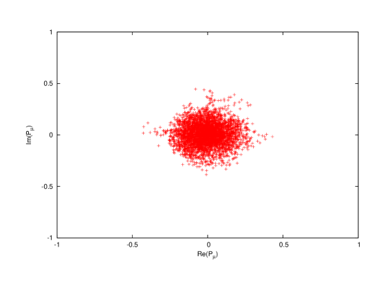
Figure 1: A traced Polyakov loop distribution that only has a central lump: $N=6$, $b=0$, $m=0.0001$.

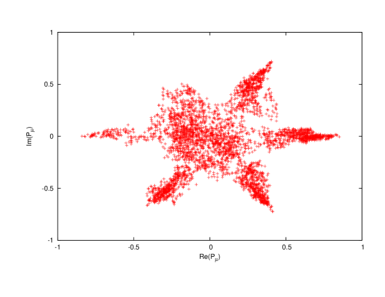
Figure 2: A traced Polyakov loop distribution with “fingers” $N=6$, $b=0.30$, $m=0.0001$.

It is interesting to observe what happens to the distribution of Polyakov loop values as $b$ is increased. In Fig. 4 it can be seen that for $N=3$ as $b$ is increased the Polyakov loop distribution moves out into the fingers and away from the center. Thus it becomes less and less likely that a configuration will tunnel from one of the fingers into another. This is an indication that the eigenvalue distribution of the link variables is far from uniform in the large $b$ limit.

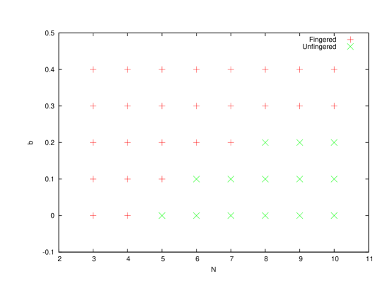
Figure 3: The “critical” values $b_{c}$, where fingers clearly form, increases with the number of colors $N$. These results are for $m=0.0001$, essentially a massless fermion.

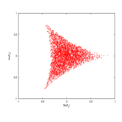
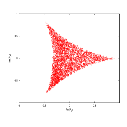
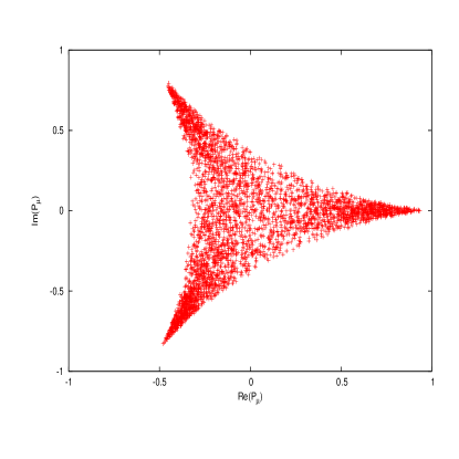
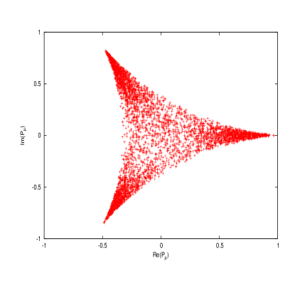
Figure 4: $N=3$ Polyakov loop distribution for increasing $b$ values. In the upper left-hand panel is shown $b=0.00$, in the upper right $b=0.10$, in the lower left $b=0.20$ and in the lower right $b=0.30$. It can be seen that the values are tending to move further out into the three fingers, and away from the center, as $b$ is increased.

V Eigenvalue analysis

If the eigenvalues of the untraced Polyakov loop operator have a uniform distribution in the $N\to\infty$ limit, then the theory is certainly center symmetric. These eigenvalues lie on the unit circle in the complex plane, and are thus of the form $e^{i\theta}$.

V.1 Unquenched theory

V.1.1 Zero mass

In our analysis for zero mass ($m=0.0001$ in practice), the eigenvalue distribution is fit to the following form:

$$F(\theta)=A+B\cos(N\theta)+C\cos(2N\theta)$$ (9)

In some cases we can set $C\equiv 0$ and still get a good fit; in others, the $C$ term is necessary. When $C\equiv 0$, the ratio that we measure to test uniformity is

$$R=\left|\frac{B}{A}\right|$$ (10)

When $C\not=0$, the ratio instead is taken to be

$$R=\sqrt{\left(\frac{B}{A}\right)^{2}+\left(\frac{C}{A}\right)^{2}}$$ (11)

Since we only expect the distribution to become uniform in the $N\to\infty$ limit, the important thing is how $R$ depends on $N$. Thus we fit the ratio to

$$R(N)=c_{0}+\frac{c_{-1}}{N}+\frac{c_{-2}}{N^{2}}+\cdots$$ (12)

and find good agreement for each value of $b$; of course the coefficients depend on $b$.

A comment here is in order. In (12) we fit the data to a smooth function of $N$. However in the phase diagram Fig. 3 we make a binary distinction between fingered and unfingered. In fact as one moves toward increasing $N$ at fixed $b$, the fingers gradually shrink and eventually one ends up with a central blob. Thus the transition is in this sense smooth, and the classification into fingered and unfingered does not reflect a discontinuity. Indeed, it is a crossover behavior, and the “critical” $b_{c}$ does not indicate a singularity of any kind.

For $b=0.10$, only $N=3$ required the three parameter fit (9). For all other values of $N$ we were able to set $C=0$ and obtain a good fit. Examples are shown in Figs. 5 and 6. The subsequent fit to (12) is shown in Fig. 7, with the fit parameters obtained displayed in Table 1. The value of the constant term $c_{0}$ is consistent with zero, indicating that the eigenvalue distribution becomes uniform in the large $N$ limit. Thus we find that the center symmetry is certainly unbroken in the thermodynamic limit in the case of $b=0.10$.

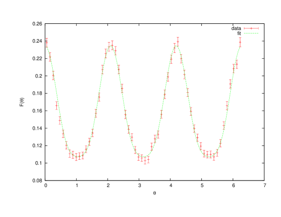
Figure 5: Eigenvalue distribution for $N=3$, $b=0.10$, $m=0.0001$, and three parameter fit (9). The $\chi^{2}/\text{d.o.f.}$ was $1.04$. Errors in the eigenvalue distribution were estimated with jackknife elimination of blocks of size 500.

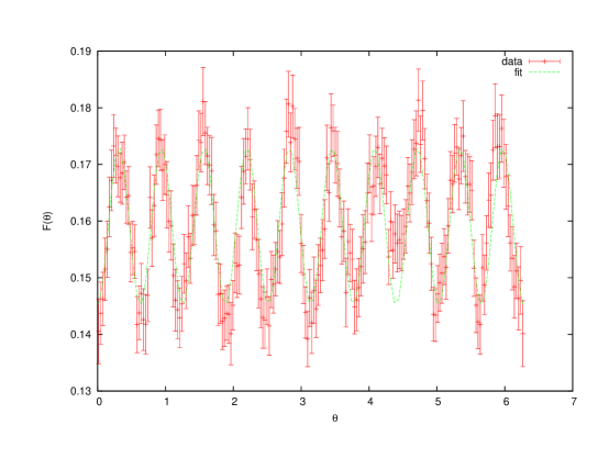
Figure 6: Eigenvalue distribution for $N=10$, $b=0.10$, $m=0.0001$, and three parameter fit (9) with $C\equiv 0$. The $\chi^{2}/\text{d.o.f.}$ was $0.96$. Errors in the eigenvalue distribution were estimated with jackknife elimination of blocks of size 500.

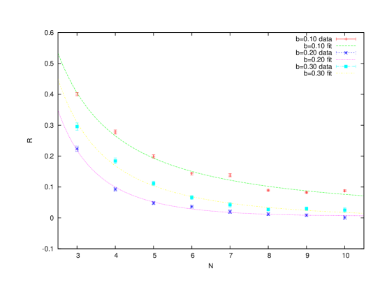
Figure 7: The ratios (10) or (11) versus $N$, and the fits, for $b=0.10,0.20$ and $0.30$. Fit results are summarized in Table 1. All three curves appear to tend toward zero in the large $N$ limit, corresponding to a uniform distribution. This is indicative of unbroken center symmetry in the thermodynamic limit.

$b$	$c_{0}$	$c_{-1}$	$c_{-2}$	$\chi^{2}/\text{d.o.f.}$
0.10	-0.006(38)	0.65(43)	1.8(1.0)	3.16
0.20	0.033(17)	-0.60(19)	3.48(46)	1.08
0.30	-0.011(5)	—	2.88(14)	1.64

Table 1: Results of fits of the ratios (10) and (11) to (12). In the case of $b=0.30$ we are able to set $c_{-1}=0$. All three fits give results that are $\sim 2\sigma$ consistent with a uniform distribution in the large $N$ limit.

For $b=0.20$, data for $N=3,\dots,7$ required all three parameters in (9), whereas for $N=8,9,10$ we were able to set $C\equiv 0$, since the two parameter fit was acceptable and $C$ was very small if it was included. The fit to (12) is shown in Fig. 7, and the fit parameters are tabulated in the second row of Table 1. The value of the constant term, $c_{0}$, is $1.9\sigma$ from zero, which we view as most likely consistent with a uniform distribution in the large $N$ limit, given the uncertainties in the measurement [e.g., a fairly simple-minded functional form has been assumed in (9).] Thus we conclude that for $b=0.20$, the center symmetry is probably unbroken in the thermodynamic limit.

For $b=0.30$, the fits to the eigenvalue distribution required three parameters: The ratio (11) was then fit to (12) with $c_{-1}\equiv 0$ since it was found that a $1/N$ term did not improve the fit. The result was row three of Table 1, and shown in Fig. 7. Since a negative value in the $N\to\infty$ limit is actually excluded by the positive definite form of $R$, it is clear that the value of $c_{0}$ is merely a fitting error; the interpretation is that it is actually zero, since it is close to zero ($2.2\sigma$), consistent with a uniform distribution in the $N\to\infty$ limit. We therefore conclude that for $b=0.30$, the center symmetry is most likely unbroken in the thermodynamic limit.

We were unable to obtain reliable results for the eigenvalue distribution for larger values of $b$ because the acceptance rates in the simulation are tending to zero, forcing very small moves, which leads to enormous autocorrelation times and incomplete sampling. The eigenvalue distributions require many more statistically independent samples in order to get good fits than does the analysis of whether or not the traced Polyakov loop has fingers, which is why we were only able to go to $b=0.30$ in the former case but were able to go to $b=0.40$ in the latter case. This is also true of the ${\tilde{P}}_{\mu}$ observable considered below in Sec. VI. All the values of $b$ that we have been able to examine in this massless case indicate a center symmetric phase in the large $N$ limit. We thus conclude that there is no evidence of center symmetry breaking from the perspective of the eigenvalue distribution in the massless theory.

V.1.2 Nonzero mass

In order to provide some contrast, we next consider the case of nonzero mass. If the mass is large enough, we should recover the quenched result of center symmetry breaking starting around $b\sim 0.15$. For $b=0.05$ and $m=0.1$, we find the two parameter fit to the distribution is successful, and that the ratio must be fit to

$$R(N)=c_{0}+c_{-2}N^{-2}+c_{-3}N^{-3}$$ (13)

in order to get good agreement with the data. The result is

$$c_{0}=0.081(3),\quad c_{-2}=8.8(3),\quad c_{-3}=-13.4(8),\quad\chi^{2}/\text{d.o.f.}=1.69$$ (14)

and the data and fit are displayed together in Fig. 8. The constant term (corresponding to the $N\to\infty$ limit) is significantly nonzero when taking into account the error of the fit. A nonuniform distribution in the large $N$ limit is clearly indicated.

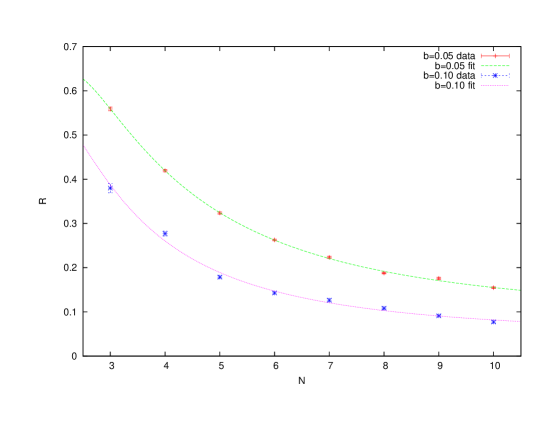
Figure 8: The ratios versus $N$, and the fits, for $b=0.05,0.10$ and $m=0.1$.

We have also looked at larger $b$ to see if this signal of a nonuniform distribution strengthens. For this purpose we studied $b=0.10$. In that case our best fit occurs with

$$R(N)=c_{0}+c_{-2}N^{-2}+c_{-4}N^{-4}$$ (15)

with

$$c_{0}=0.043(8),\quad c_{-2}=4.0(5),\quad c_{-4}=-8(5),\quad\chi^{2}/\text{d.o.f.}=4.9$$ (16)

The data and fit are shown in Fig. 8. While the $\chi^{2}/\text{d.o.f.}$ is not very good, we find the nonzero value of $c_{0}$ to be robust with respect to other choices of fit. The data seem to indicate that also for this value of $b$, there is a nonuniform distribution in the limit of infinite $N$, though the conclusion is not any stronger.

Moving to $b=0.20$, fits based on (9) no longer work well, missing other modes that are apparent in the data. The eigenvalue distribution requires a more sophistocated fitting procedure which we now explain. We have used $20N$ bins, with boundaries at

$$\theta_{j}=j\frac{\pi}{10N}$$ (17)

so that correspondingly we have distribution heights $f_{j}=f(\theta_{j})$. Next we perform a discrete Fourier transform of this function to obtain ${\tilde{f}}_{k}$, taking into account that $f_{j}$ is real (we use FFTW Frigo (1999) for this). Naturally we find the amplitude $|{\tilde{f}}_{0}|$ to be by far the largest, corresponding to the constant mode. Next we sort the amplitudes into descending order,

$$|{\tilde{f}}_{k_{0}}|>|{\tilde{f}}_{k_{1}}|>\cdots>|{\tilde{f}}_{k_{n}}|>\cdots$$ (18)

An example of the amplitudes versus $k$ is shown in Fig. 9. We then fit the distribution to

$$F(\theta)=a_{0}+a_{1}\cos(k_{1}\theta+b_{1})+a_{2}\cos(k_{2}\theta+b_{2})+\cdots+a_{n}\cos(k_{n}\theta+b_{n})$$ (19)

An example is displayed in Fig. 10. For $b=0.05$ and $0.10$ we find that $n=5$ is sufficient, and in fact $n=6$ fails for $b=0.10$ in that one of the coefficients has over 100% error. For $b=0.20$ and $0.30$ we find that the fits are improved by taking $n=6$. In either case the ratio is computed from

$$R=\left[\left(\frac{a_{1}}{a_{0}}\right)^{2}+\cdots+\left(\frac{a_{n}}{a_{0}}\right)^{2}\right]$$ (20)

which is an obvious generalization of (11). The results are shown in Fig. 11. Fit results are given in Table 2.

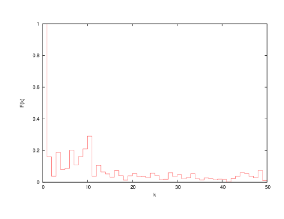
Figure 9: Example of the distribution of $F(k)\equiv|{\tilde{f}_{k}}|$ for $N=5$, $b=0.20$, $m=0.1$. Note that $F(0)=15.9$ extends out of the field of view, in order to show the other, much smaller values.

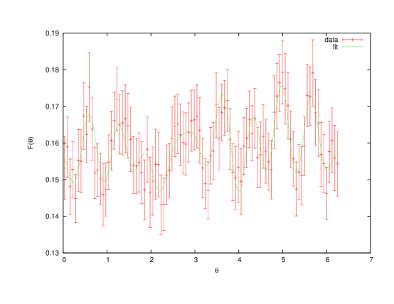
Figure 10: Example of the fit to the eigenvalue distribution using Eq. (19) for $N=5$, $b=0.20$, $m=0.1$. Here, $n=6$, the six leading nonzero modes shown in Fig. 9, in addition to the constant $k=0$ mode.

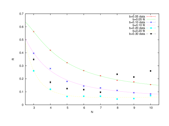
Figure 11: The ratio (20) versus $N$, and the fit, for $b=0.05,0.10,0.20,0.30$, $m=0.1$, using the Fourier transform method. Here $n=5$ for $b=0.05,0.10$ and $n=6$ for $b=0.20,0.30$.

$b$	$c_{p_{1}}$	$c_{p_{2}}$	$c_{p_{3}}$	$\chi^{2}/\text{d.o.f.}$	$(p_{1},p_{2},p_{3})$
0.05	0.0835(35)	8.58(29)	-12.81(84)	2.58	(0,2,3)
0.10	0.0482(79)	3.78(44)	-5.6(3.9)	8.23	(0,2,4)
0.20	0.071(13)	-2.48(99)	12.6(2.9)	7.27	(0,2,3)

Table 2: Ratio fit results when the Fourier transform method and $n=5$ or $6$ is used. We use either (13) or (15) for the form of $R(N)$, denoted by the powers $(p_{1},p_{2},p_{3})$ in the last column. No fit is performed for $b=0.30$, because as can be seen from Fig. 11 the $N=8,9,10$ results break away from the trend at smaller $N$.

For the cases of $b=0.05,0.10,0.20$ we find that the fit indicates that the eigenvalue distribution is not uniform in the large $N$ limit, in the first two cases consistent with findings described in previous paragraphs that did not use the Fourier transform method. In the case of $b=0.30$, we cannot fit to either of the forms (13) or (15) because there is a jump in the behavior at $N=8$. This significant nonuniformity at large $N$ is consistent with what is seen in the quenched case considered below for $b>0.15$. Thus it appears that the quenched behavior of center symmetry breaking at large $N$ is obtained for this large mass of $m=0.1$ when $b\mathrel{\hbox to0.0pt{\raise 2.15277pt\hbox{$>$}\hss}{\lower 2.15277pt\hbox{$\sim$}}}0.20$. It is reasonable to assume that the $b$ value for which this begins to occur is somewhat larger than in the quenched case for a finite mass $m$, as compared to $m\to\infty$, where the quenched transition of $b\sim 0.15$ would occur.

V.2 Quenched theory

For purposes of further comparison, we have also analyzed the eigenvalue distribution in the quenched theory (i.e., setting the fermion determinant to unity). The eigenvalue distribution was found to have a few different forms, in contrast to the massless unquenched case where (9) always worked. The other forms that were required were

$$F(\theta)=A+B\cos(2N\theta)+C\cos(\theta+D)$$ (21)

and (9) with $B=0$. In some cases we could also set $B=0$ or $D=0$ in (21) and obtain a good fit (the parameter dropped was consistent with zero if it was included). Two examples of these different shapes are shown in Figs. 12 and 13.

We believe that it is significant that the $N$-fold periodicity of (9) is lost and replaced with (21), $C\not=0$, for those values of $b$ that seem to have broken center symmetry in the large $N$ limit according to the detailed analysis below. For $b=0.2$ the alternative form (21) must be used for $N\geq 6$, for $b=0.3$ it must be used for $N=4$ and $N\geq 6$, and for $0.4$ it must be used for $N\geq 4$. Thus the breakdown in $N$-fold periodicity occurs at smaller and smaller $N$ as $b$ increases, corresponding to a more dramatic violation of center symmetry. This also correlates with the fact that in the massive unquenched case of $b\geq 0.20$ it was necessary to use more general forms (19).

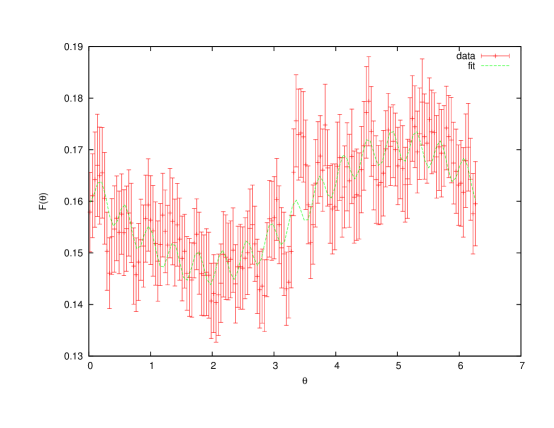
Figure 12: Quenched theory eigenvalue distribution for $b=0.3$, $N=8$, fit to (21). The goodness of the fit was $\chi^{2}/\text{d.o.f.}=0.40$. Comparing to Fig. 6, it can be seen that for the quenched theory at large $N$ with $b$ greater than the critical value there is a drastic change in the eigenvalue distribution.

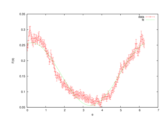
Figure 13: Quenched theory eigenvalue distribution for $b=0.4$, $N=8$, fit to (21) with $B=0$. The goodness of the fit was $\chi^{2}/\text{d.o.f.}=2.17$.

After the fits were performed, ratios were then formed using either (10) (with $B\to C$ in the case where $B=0$) or (11) (ignoring the parameter $D$ when (21) was used). The results are shown in Figs. 14 and 15. Whereas for $b=0.10$ there is a clear decrease with increasing $N$, for the larger values of $b$ the trend at large $N$ is either to a constant nonuniformity or one that is rapidly increasing. Naturally this strengthens as $b$ is pushed to larger values.

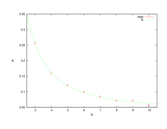
Figure 14: Quenched $b=0.10$ ratio versus $N$. There is a clear decrease with increasing $N$.

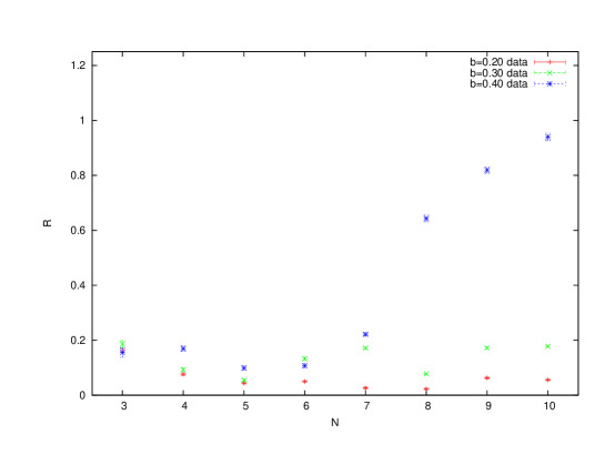
Figure 15: Quenched $b=0.20,0.30,0.40$ ratio versus $N$. The ratio either approaches a constant value significantly different from zero, or shows an increasing trend with $N$. Clearly there is a dramatic change for $b\geq 0.40$.

Fitting the ratio versus $N$ for $b=0.1$, using the form

$$R(N)=c_{0}+c_{-2}N^{-2}$$ (22)

gives

$$c_{0}=0.0438(22),\quad c_{-2}=1.909(57),\quad\chi^{2}/\text{d.o.f.}=4.88$$ (23)

We attempted other more general forms of $N$ dependence; none of these reduced the $\chi^{2}/\text{d.o.f.}$. However, there is a clear decrease with $N$ to a small constant in the large $N$ limit. Thus the eigenvalue distribution becomes to a very good approximation uniform in the large $N$ limit. It will be argued in Section VII below that this is an indication of unbroken center symmetry. This is also consistent with old results such as Bhanot et al. (1982) that place $b=0.10$ below the transition.

By contrast, for $b=0.20,0.30,0.40$ we cannot fit any smooth function to the data, so it is not possible to extrapolate to large $N$. The most that can be said is that the ratio tends to a small value for $b=0.20$ and a relatively large value $\sim 0.2$ for $b=0.30$. For $b=0.40$ the ratio is monotonically increasing at large $N$, reaching quite large values $\sim 1.0$. For purposes of comparison, Ref. Bhanot et al. (1982) examined $N=5$ and found fluctuations in the free energy between quadratic and quartic behavior for what is $b\geq 0.15$ in our language. They interpreted this as evidence for symmetry breaking. This suggests that the irregular behavior we see in Fig. 15 is a precursor to spontaneous symmetry breaking in the large $N$ limit.

The conclusion we draw is that in the quenched theory $b=0.10$ is certainly center symmetric and $b=0.40$ is certainly broken in the thermodynamic limit of a large number of colors. An irregular behavior and significant large $N$ nonuniformity occurs for $b=0.2$ and $b=0.3$, which is consistent with symmetry breaking in the large $N$ limit. Looking at the size of the fluctuations in the eigenvalue spectrum relative to the constant part gives a powerful way to distinguish between, in particular, the two cases of $b=0.10$ and $b=0.40$. Intermediate values of $b$ are harder to differentiate.

VI ${\tilde{P}}_{\mu}$ observable

In this section we consider the observable in Eq. (4) above, which has been used in previous study Hietanen and Narayanan (2012). We will find that it is not decisive in identifying center symmetry breaking, because it is difficult to make a binary distinction based on the value of this quantity. Indeed we will find that the ratio obtained in the previous section is a much more reliable indicator, and that the values of ${\tilde{P}}_{\mu}$ are merely supportive of the conclusions reached by that approach, in a suggestive way.

VI.1 Unquenched theory

One advantage of the ${\tilde{P}}_{\mu}$ observable is that it is obtained with high accuracy from the simulations, as can be seen in Fig. 16. Indeed, the error bars (estimated with jackknife block elimination as before) are barely visible. In this figure we show ${\tilde{P}}_{\mu}$ for four values of $b$ (in this case $b=0.4$ was possible because the observable has far smaller fluctuation than the eigenvalue distributions of the previous section) in the approximately massless case of $m=0.0001$. We have fit the data to

$$A+BN^{-2}+CN^{-4}$$ (24)

and in all cases obtain reasonably good agreement, as can be seen in Table 3.

b	A	B	C	$\chi^{2}/\text{d.o.f.}$
0.10	0.49983(63)	-0.927(44)	1.55(41)	1.91
0.20	0.4767(17)	-1.308(83)	3.16(69)	1.55
0.30	0.4223(11)	-1.113(61)	2.79(49)	0.88
0.40	0.38080(98)	-0.901(53)	1.72(42)	0.71

Table 3: Fit results for ${\tilde{P}}_{\mu}$ in the unquenched theory with $m=0.0001$, comparing data to Eq. (24).

Figure 16: ${\tilde{P}}_{\mu}$ versus the number of colors $N$ for various values of the inverse ’t Hooft coupling $b$, with $m=0.0001$. It can be seen that as $b$ is increased, the distribution of Polyakov loops becomes less central in the large $N$ limit, pushing ${\tilde{P}}_{\mu}$ away from $1/2$.

The large $N$ limiting behavior of ${\tilde{P}}_{\mu}$ is given by the coefficient $A$. It can be seen that this quantity declines as $b$ is increased, indicating that the data for the Polyakov loop is spreading out away from the origin in the complex plane and is becoming less central. However, it is impossible to tell from ${\tilde{P}}_{\mu}$ whether or not barriers are emerging between the $N$ vacua, so one cannot draw a firm conclusion about spontaneous center symmetry breaking. In fact, since the eigenvalue analysis above indicated that center symmetry is not broken in the unquenched case, a consistent interpretation would require that the decrease in ${\tilde{P}}_{\mu}$ is not related to barrier formation, but only a less centralized distribution in the Polyakov loop which still allows tunneling in the large $N$ limit, destroying any putative order.

We have also computed ${\tilde{P}}_{\mu}$ for the massive case $m=0.1$ that was considered previously, with results shown in Fig. 17. Comparing the $b=0.10$ entry of Table 4 to the $b=0.10$ entry of Table 3 it can be seen that the mass has little effect on the ${\tilde{P}}_{\mu}$ observable in the large $N$ limit for small values of $b$. Both $b=0.05$ and $b=0.10$ with the large mass $m=0.1$ extrapolate to $1/2$ to a very good approximation in the large $N$ limit, indicating an absence of spontaneous symmetry breaking. We also see that the large $N$ limit, given by the coefficient $A$, is quite similar between the massless and massive cases for $b=0.20,0.30$. The eigenvalue analysis indicated that $b=0.30$ was most likely broken, and there was a clear distinction between that behavor for $m=0.0001$ versus $m=0.1$. By contrast the ${\tilde{P}}_{\mu}$ observable does not really allow for a way to differentiate between the massless versus large mass scenario in this regime where we expect that the center symmetry is spontaneously broken in the latter case.

b	A	B	C	$\chi^{2}/\text{d.o.f.}$
0.05	0.49988(24)	-0.616(17)	0.25(16)	1.53
0.10	0.49978(55)	-0.928(38)	1.45(36)	2.40
0.20	0.4784(16)	-1.470(91)	4.44(77)	1.70
0.30	0.4175(18)	-0.90(11)	0.85(92)	1.74

Table 4: Fit results for the unquenched theory with $m=0.1$, comparing data to Eq. (24).

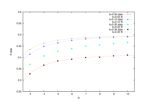
Figure 17: ${\tilde{P}}_{\mu}$ versus the number of colors $N$ for the inverse ’t Hooft coupling $b=0.05,0.10,0.20,0.30$ that we ran with $m=0.1$.

VI.2 Quenched theory

As in Section V, we now contrast with the quenched theory, where it is well-known that the symmetry is broken for sufficiently large values of $b$. The results are summarized in Fig. 18. Comparing to Fig. 16, what one sees is that there is a significant difference in behavior between $b=0.10,0.20$ versus $b=0.30,0.40$ in the quenched case, which did not occur in the unquenched case. The latter two values of $b$ are significantly lower and actually trend somewhat downward as $N$ is increased. The fits to (24) are shown in Table 5; the $b=0.40$ case does not give a good fit, but it is clear that the asymptotic value in the large $N$ limit is significantly smaller than in the unquenched case. Setting aside the poor quality of the fit in this case, the large $N$ limit of $A=0.2939(38)$ for $b=0.40$ is far below the value in the highly symmetric case of $b=0.10$, $A=0.50074(30)$ which is essentially $1/2$. This is indicative of the strong breaking of center symmetry for this large value of $b=0.4$, as usual in the large $N$ limit.

b	A	B	C	$\chi^{2}/\text{d.o.f.}$
0.10	0.50074(30)	-1.177(22)	2.12(22)	1.53
0.20	0.4425(13)	-1.147(66)	2.55(57)	1.75
0.30	0.3511(17)	0.175(96)	-4.40(81)	2.20
0.40	0.2939(38)	0.91(22)	-7.8(1.8)	4.21

Table 5: Results for the fit of the quenched data to Eq. (24).

Figure 18: ${\tilde{P}}_{\mu}$ versus the number of colors $N$ for various values of the inverse t’ Hooft coupling $b$ in the quenched case. The values for large $N$ (i.e., the value of $A$) are consistent with center symmetry breaking in the cases of $b=0.30$ and $0.40$.

VII Spontaneous symmetry breaking for the single site lattice

There is a free energy of the (traced) Polyakov loop $P$, $F_{N}(P)$, for each value of $N$. Spontaneous symmetry breaking would mean that there is a very large barrier between the $N$ different minima of $F_{N}(P)$, because otherwise the finite tunneling probability would destroy any order. In fact, this is the reason why the thermodynamic limit must be taken in order to have true spontaneous symmetry breaking, because we need a very large number of degrees of freedom in order to produce the corresponding large barriers. These barriers can only arise in the thermodynamic limit, which is formally $N\to\infty$ in the single site lattice theory. It follows that the vacua are quite close to each other in the relevant limit, so the vanishingly small tunneling between them is a subtle issue. It is necessary for the distribution of $\arg(P)$ to become highly nonuniform in the thermodynamic limit. The point is that on the single site lattice there is a free energy density, $f_{N}(P)=F_{N}(P)/N^{2}$, which is a reasonable function, but

$$\exp(-F_{N}(P))=\exp(-N^{2}f_{N}(P))$$ (25)

gets vanishingly small weight at all but the minima of $f_{N}(P)$ in the large $N$ limit. Any external perturbation will then freeze it into one of those minima, and the barrier for tunneling is effectively infinite.

This discussion makes it clear that the physics of spontaneous symmetry breaking in the single site lattice theory must be understood in the large $N$ limit. It is for this reason that we have studied a method that allows for an $N\to\infty$ extrapolation in the previous section. Certainly a vanishing ratio (10) or (11) would be a clear indication of a uniform distribution, and hence no spontaneous symmetry breaking. However, from our understanding of spontaneous symmetry breaking as arising from infinite barriers, we see that small but finite ratio (such as was found for $b=0.10$ in the $m=0.1$ case) does not indicate a broken symmetry phase, since there is still a finite density of states in the tunneling region that lies between the vacua. Indeed, the ratio should become rather large if the symmetry is spontaneously broken in the $N\to\infty$ limit. Correspondingly, a fingered traced Polyakov loop distribution is not a clear indicator of a broken phase, since there still is a nonzero density of states in the central tunneling region. Only in the case where multiple observables indicate a high degree of nonuniformity in the thermodynamic limit can one conclude with any confidence that center symmetry is spontaneously broken. Examples of this are the unquenched theory with $b=0.30$ and $m=0.1$, or the quenched theory with $b=0.30,0.40$.

VIII Conclusions

We have found that on the single site lattice with Ginsparg-Wilson-type fermions (in our case Möbius), center symmetry is unbroken in the large $N$ limit if the fermions are effectively massless. On the other hand, at the relatively large mass value of $m=0.1$, we find that sufficiently large $b$ will induce spontaneous center symmetry breaking at large $N$. This agrees with the fact that in the continuum large $N$ limit the one loop effective potential for the eigenvalues of the (untraced) Polyakov loop shows that they repel and are uniformly distributed for any $N_{f}\not=0$ Kovtun et al. (2007), provided the fermions are massless.

A different result has been obtained recently using an approach which truncates the link matrices to diagonal matrices only consisting of their eigenvalues, finding that in the large $N$ limit, $N_{f}=1$ has spontaneously broken center symmetry Lohmayer and Narayanan (2013). It may be that this truncation somehow misses important physics. Our nonperturbative lattice results agree with Ref. Hietanen and Narayanan (2012) which found that to a good approximation (4) was $1/2$, corresponding to Polyakov loops near zero on most configurations, and hence unbroken center symmetry. Similarly, the older study Bringoltz and Sharpe (2009) which used Wilson fermions found unbroken center symmetry for a wide range of fermion masses. We believe that our present study goes beyond these results by fitting the eigenvalue distribution to a function of $N$ so that the large $N$ limit can be taken. Since true spontaneous symmetry breaking can only be obtained in this limit, we would argue that it is important to develop a quantitative method that is amenable to such an extrapolation. We have also presented an argument that simply having a nonuniform distribution does not necessarily imple spontaneous symmetry breaking, since one must consider the possibility of tunneling between the $N$ ground states in the large $N$ limit. By comparing to the quenched case, where the fate of center symmetry is understood, we have concluded that the nonuniformity must be rather large.

Our simulation results also agree with the nonperturbative findings of Hietanen and Narayanan (2010, 2011), where the theory of a single Majorana fermion (“half a Dirac flavor”) in the adjoint representation was studied on a single site lattice. For $N=11$ and $b=7$ they found in Hietanen and Narayanan (2010) that the quantity (4) was approximately $1/2$ for the right range of the Wilson kernel mass (what we are calling $m_{5}$). In Hietanen and Narayanan (2011) they found that for $N=11,15$ and $18$ the quantity (4) was approximately $1/2$ for $b=5$, provided the fermion mass $m$ in lattice units satisfied $m<0.1$.

One direction for further research is to increase the values of $b$ that we are able to probe. This would require abandoning the Metropolis algorithm in favor of something like the rational hybrid Monte Carlo algorithm.

References

- Eguchi and Kawai (1982) T. Eguchi and H. Kawai, Phys.Rev.Lett. 48, 1063 (1982).
- Bhanot et al. (1982) G. Bhanot, U. M. Heller, and H. Neuberger, Phys.Lett. B113, 47 (1982).
- Kazakov and Migdal (1982) V. Kazakov and A. A. Migdal, Phys.Lett. B116, 423 (1982).
- Kovtun et al. (2007) P. Kovtun, M. Unsal, and L. G. Yaffe, JHEP 0706, 019 (2007), arXiv:hep-th/0702021 [HEP-TH] .
- Bringoltz and Sharpe (2009) B. Bringoltz and S. R. Sharpe, Phys.Rev. D80, 065031 (2009), arXiv:0906.3538 [hep-lat] .
- Bringoltz (2009) B. Bringoltz, JHEP 0906, 091 (2009), arXiv:0905.2406 [hep-lat] .
- Hietanen and Narayanan (2012) A. Hietanen and R. Narayanan, Phys.Rev. D86, 085002 (2012), arXiv:1204.0331 [hep-lat] .
- Hietanen and Narayanan (2010) A. Hietanen and R. Narayanan, JHEP 1001, 079 (2010), arXiv:0911.2449 [hep-lat] .
- Lohmayer and Narayanan (2013) R. Lohmayer and R. Narayanan, Phys.Rev. D87, 125024 (2013), arXiv:1305.1279 [hep-lat] .
- Brower et al. (2012) R. C. Brower, H. Neff, and K. Orginos, (2012), arXiv:1206.5214 [hep-lat] .
- (11) “MAGMA: Matrix algebra on GPU and multicore architectures,” http://icl.cs.utk.edu/magma/index.html.
- Cabibbo and Marinari (1982) N. Cabibbo and E. Marinari, Phys.Lett. B119, 387 (1982).
- Okawa (1982) M. Okawa, Phys. Rev. Lett. 49, 353 (1982).
- Frigo (1999) M. Frigo, in Proceedings of the 1999 ACM SIGPLAN Conference on Programming Language Design and Implementation (PLDI ’99), Atlanta, Georgia, May 1999 (1999).
- Hietanen and Narayanan (2011) A. Hietanen and R. Narayanan, Phys.Lett. B698, 171 (2011), arXiv:1011.2150 [hep-lat] .